Modelling Exposure from Airborne Hazardous Short-Duration Releases in Urban Environments

Abstract

When considering accidental or/and deliberate releases of airborne hazardous substances the release duration is often short and in most cases not precisely known. The downstream exposure in those cases is stochastic due to ambient turbulence and strongly dependent on the release duration. Depending on the adopted modelling approach, a relatively large number of dispersion simulations may be required to assess exposure and its statistical behaviour. The present study introduces a novel approach aiming to replace the large number of the abovementioned simulation scenarios by only one simulation of a corresponding continuous release scenario and to derive the exposure-related quantities for each finite-duration release scenario by simple relationships. The present analysis was concentrated on dosages and peak concentrations as the primary parameters of concern for human health. The experimental and theoretical analysis supports the hypothesis that the dosage statistics for short releases can be correlated with the corresponding continuous release concentration statistics. The analysis shows also that the peak concentration statistics for short-duration releases in terms of ensemble average and standard deviation are well correlated with the corresponding dosage statistics. However, for more reliable quantification of the associated correlation coefficients further experimental and theoretical research is needed. The probability/cumulative density function for dosage and peak concentration can be approximated by the beta function proposed in an earlier work by the authors for continuous releases.

1. Introduction

It is well known that following a short-duration (puff) release, the airborne material that reaches a receptor downwind of the source presents high concentration variability between different realisations of the same short-duration release under the same mean flow conditions, (e.g., [1]). This is mainly due to the local conditions of turbulence which force the material to travel in different pathways in each realisation. An analysis of the experimental data (e.g., [2]) reveals that the variability is reflected on puff-related parameters such as the dosage, peak concentration, arrival time, duration etc. Thus, there is a necessity to quantify the statistical behaviour of these puff-related parameters and especially the ones that concern the human health, i.e., the dosages and the peak concentrations.

There is an important effort in the literature to simulate puff dispersion theoretically/numerically (e.g., [3,4,5,6]). Furthermore, in [7] equations are presented for recalculating the continuous-source results to achieve results valid for the short-term source. The outputs obtained were the probability density functions of the puff characteristics: dosage, maximum concentration, and 99th and 95th percentiles of concentrations.

In addition to the above mentioned variability between different realisations of the same finite-duration release under the same mean flow, for an emergency action plan there is often the need to examine several release scenarios that, among other parameters, concern the release duration itself, which is not known a priori. In computational terms this means that acting in a straightforward manner, this could lead to a relatively high number of simulations to be performed. On the other hand to model an actual exposure scenario in a complex situation such as an urban environment, the use of advanced Computational Fluid Dynamics (CFD) technology is probably the only possibility for producing reliable results.

It is noted that CFD technology is highly demanding with respect to CPU time, especially if the user considers Direct Numerical Simulation (DNS) or Large-Eddy Simulation (LES) approaches. Even for the Reynolds-Averaged Navier–Stokes (RANS) approach, the CPU time is not negligible especially when the number of scenarios to be examined is relatively high.

It is clear from the above that the problem becomes more demanding with respect to the number of simulations if one needs to consider a variety of release durations and in the same time assess the statistical behaviour of the exposure parameters connected to a specific short-duration release.

Therefore, for practical reasons, there is a need to develop simplified but reliable methodologies to cope with this complex problem.

The basic idea here is as follows. When studying release-duration scenarios we can always consider in addition the (single) continuous release scenario. The question is to what degree the exposure parameters, either deterministic or statistical, of a short/finite-duration release are related to the corresponding parameters of a properly defined “equivalent” continuous release. It is noted that the continuous release is a well-studied problem with several existing models able to produce reliable results [8,9,10,11,12,13,14,15].

Closely connected to the behaviour of exposure parameters from both continuous and short-duration atmospheric releases are concentration fluctuations. Indeed, the need to take into account concentration fluctuations in the assessment of hazards from the dispersion of substances has long been recognised (e.g., [16,17]) and concentration fluctuations have been connected to doses in e.g., [18,19]. There is an extended literature in modelling of concentration calculations. The use of analytic forms for calculating the corresponding probability density function (PDF) in open field atmospheric dispersion has been examined in, e.g., [20,21,22,23,24,25]. The use of a transport equation for the concentration variance was first adopted in [26]. Of particular interest for the present paper is the calculation of concentration fluctuations in dispersion in urban environments or in the vicinity of buildings [27,28,29,30,31,32,33,34,35,36,37,38,39]. Several experimental studies of concentration fluctuations of plume (continuous release) dispersion in urban areas or in the vicinity of buildings in real scale or in the wind tunnel have also been reported in the literature [40,41,42,43,44]. Fewer experimental investigations of concentration fluctuations in puffs from quasi-instantaneous releases have been reported (e.g., [45,46]). A recent and most comprehensive review of modelling and experimental research on concentration fluctuations to date has been presented in [47].

The main aim of the present study is to reveal for the first time relationships of exposure parameters of a short/finite-duration release with the corresponding parameters of a properly defined “equivalent” continuous release based on experimental evidence and theoretical considerations. It is noted that if this effort is successful, the benefits could be quite significant, since in most cases a relatively large number of dispersion simulations, reflecting the variety of potential release duration scenarios as well as its stochastic dispersion behaviour, can be replaced by a single continuous release simulation.

The paper presents also experimental evidence that the peak concentration statistics for short-duration releases in terms of ensemble average and standard deviation are well correlated with the corresponding dosage statistics. Finally, the paper presents experimental evidence that the probability/cumulative density function for dosage and peak concentration can be approximated by the beta function proposed in an earlier work by the authors for continuous releases.

The structure of the paper is as follows:

• Statement of the hypotheses connecting the short-release ensemble average dosage and its standard deviation with the corresponding continuous-release mean concentration and its standard deviation (Section 2).
• Theoretical establishment of the relationship between short duration release ensemble average dosage and corresponding continuous release mean steady-state concentration (Section 2.1).
• Theoretical establishment of the relationship between short duration release dosage standard deviation and corresponding continuous release concentration standard deviation (Section 2.2).
• Experimental evidence in support of the proposed relationships (Section 3.1).
• Experimental evidence of the relationship between peak concentration and dosage statistics for short-duration releases (Section 3.2).
• Experimental evidence supporting that the probability/cumulative density function for puff ensemble average dosage and peak concentration can be approximated by the beta function (Section 3.3).
• Conclusions (Section 4).

2. Methodology

Let us assume a point source at a given location, releasing a total quantity $QT \left[kg\right]$ of a hazardous pollutant within a finite time duration $∆T \left[s\right]$. In this case the corresponding emission rate $Q$ $\left[kg·s^{-1}\right]$ is given by the relation:

$$Q=\frac{QT}{∆T}$$

(1)

For a finite-duration release, the dosage $D \left[kg·s·m^{-3} \right]$ at a receptor point downstream is defined here as the concentration time integral:

$$D={{\displaystyle \int }}_0^{\infty }C\left(t\right) dt$$

(2)

where $C\left(t\right) \left[kg·m^{-3}\right]$ is the concentration time series at the receptor point. The integration time beyond $∆T$ reflects the increase in cloud passage time due to diffusion processes.

It is noted that if $∆T$ falls well within the ambient turbulence time period’s range, the dosage $D$, by integrating different turbulence time periods for each realisation, is expected to have an inherent variability translating to a stochastic behaviour. The problem is to quantify at any receptor point this dosage statistic in terms of the ensemble average $\overline{D}$, its standard deviation ${\sigma }_D \left[kg·s·m^{-3} \right]$ and the appropriate probability/cumulative density function (pdf/cdf). The ensemble here is composed by different dispersion realisations of the release with duration $∆T$.

Let us in parallel consider the supplementary problem of a continuous release of the same release rate $Q$ which generates at the same receptor point the concentration time series $CS\left(t\right) \left[kg·m^{-3}\right]$. In principle this time series is infinite in length. If we randomly extract from this time series a piece of time-length $∆T$, we can calculate a corresponding dosage $DS \left[kg·s·m^{-3} \right]$ as

$$DS={{\displaystyle \int }}_{\Delta {\rm T}}^{}CS\left(t\right)dt=CS\left(∆T\right) ∆T$$

(3)

where $CS\left(∆T\right)$ is the time-averaged concentration over $∆T$. Both $DS$ and $CS\left(∆T\right)$ are stochastic variables. The $DS$ statistical behavior is directly connected to the $CS\left(∆T\right)$ statistical behavior. Let $\overline{CS}\left(∆T\right)$ and ${\sigma }_{CS}\left(∆T\right) \left[kg·m^{-3}\right]$ be the mean and standard deviation of $CS\left(∆T\right),$ respectively. As $\overline{CS}\left(∆T\right)$ is calculated by drawing a relatively large number of “samples” of length $∆T$ from the infinite time series $CS\left(t\right)$, it follows that

$$\overline{CS}\left(∆T\right)\approx \overline{CS}$$

(4)

where on the right-hand side $\overline{CS}=\overline{CS}(\infty )$ is the mean steady-state concentration of the continuous release at the receptor location.

In this study we introduce the hypotheses that the short-release ensemble average dosage $\overline{D}$ and its standard deviation ${\sigma }_D$ are directly related to the corresponding continuous-release mean concentration $\overline{CS}$ and its standard deviation ${\sigma }_{CS}\left(∆T\right),$ respectively, as follows:

$$\frac{\overline{D}}{QT}\approx {\alpha }_m\frac{\overline{CS}}{Q}$$

(5)

and

$$\frac{{\sigma }_D}{QT}\approx {\alpha }_{\sigma }\frac{{\sigma }_{CS}\left(\Delta {\rm T}\right)}{Q}$$

(6)

The present emphasis is to test the validity of the above relationships and give a first estimate of the associated coefficients ${\alpha }_m$ and ${\alpha }_{\sigma }$.

It is noted that the above hypotheses are proposed to be valid under any source-to-sensor relative location, wind characteristics and local topography. Some inherent uncertainties on the $a_m$ and $a_{\sigma }$ values are expected due to those characteristics’ differentiation. Future extensive targeted studies will be needed to quantify such uncertainties.

2.1. Finite Duration Release Ensemble Average Dosage ($\overline{D}$) vs. Corresponding Continuous Release Mean Steady-State Concentration ($\overline{CS}$)

It is noted that in the remainder, when we refer to a concentration/dosage we mean the excess concentration/dosage that is generated solely from the above-mentioned source, i.e., above background. In other words, the background concentration is considered to be zero.

Following the relatively simple CFD-RANS approach and the eddy viscosity/diffusivity concept (e.g., [48]), the transport equation for the pollutant concentration ensemble average $\overline{C}\left(t\right) \left[kg m^{-3}\right]$ for a finite duration release, taking into consideration Equation (1), can be expressed as follows:

$$\frac{\partial }{\partial t}\left(\overline{C}\left(t\right)\right)+\frac{\partial }{\partial x_i}\left(U_i\overline{C}\left(t\right)\right)=\frac{\partial }{\partial x_i}\left(\left({{\rm K}}_d+K_{ci}\right)\frac{\partial \overline{C}\left(t\right)}{\partial x_i}\right)+Q·\delta \left(\overline{r}-\overline{r_0}\right)$$

(7)

where $U_i \left[m·s^{-1}\right]$ are the mean velocity components, $K_d \left[m^2·s^{-1}\right]$ is the molecular diffusivity and $K_{ci} \left[m^2·s^{-1}\right]$ the turbulent eddy diffusivities.

For a finite-duration release, it is reasonable to approximate the ensemble average dosage $\overline{D}$ at a receptor by the relation

$$\overline{D}={{\displaystyle \int }}_0^{\infty }\overline{C}\left(t\right)dt$$

(8)

By analogy, the mean dosage for the corresponding continuous release for a time interval $∆T$, taking into consideration Equations (3) and (4), would be given by:

$$\overline{DS}=\overline{CS}\left(\Delta {\rm T}\right) \Delta {\rm T}=\overline{CS} ∆T$$

(9)

On the other hand, the transport equation for $\overline{D}$ could be directly derived by integrating Equation (7) over time and taking into consideration Equations (8) and (1):

$$\frac{\partial }{\partial x_i}\left(U_i\overline{D}\right)=\frac{\partial }{\partial x_i}\left(\left({{\rm K}}_d+K_{ci}\right)\frac{\partial \overline{D}}{\partial x_i}\right)+QT·\delta \left(\overline{r}-\overline{r_0}\right)$$

(10)

For a continuous source, the governing transport equation for the steady state concentration $\overline{CS}$ is given by the relationship:

$$\frac{\partial }{\partial x_i}\left(U_i\overline{CS}\right)=\frac{\partial }{\partial x_i}\left(\left({{\rm K}}_d+K_{ci}\right)\frac{\partial \overline{CS}}{\partial x_i}\right)+Q·\delta \left(\overline{r}-\overline{r_0}\right)$$

(11)

We notice that if we replace $\overline{D}=\overline{CS} ∆T$ in Equation (10) we end up exactly with Equation (11). In other words, if a spatial function $\overline{CS}$ is a solution for Equation (11), the function $\overline{D}=\overline{CS}·∆T$ is a solution for Equation (10). This provides the linkage between the ensemble average dosage ($\overline{D}$) from a finite duration release with the steady-state concentration $\left(\overline{CS}\right)$ from the continuous release. Normalising the relationship $\overline{D}=\overline{CS}·\Delta {\rm T}$ by the source release mass $QT$ and taking into consideration Equation (1), we end up with the following relationship between $\overline{D}$ and $\overline{CS}$:

$$\frac{\overline{D}}{QT}=\frac{\overline{CS}}{Q}$$

(12)

Comparing Equation (12) with Equation (5) we conclude that the above relevant hypothesis is valid with the associated coefficient ${\alpha }_m$ equal to unity. In other words, Equation (12) can be used to estimate the dosage ensemble average at any receptor point caused by a source described by Equation (1) for any release duration provided that the corresponding steady state concentration has been quantified by solving Equation (11).

It is worth underlining here that with only one (steady-state) simulation we are able to estimate the ensemble average dosages for any release duration by using Equation (12).

At this point it should be underlined that the derivation of Equation (12) was possible assuming that the RANS approximation is valid. Thus, in the real problem, the relation (12) could serve as an indicator to what degree RANS approximation is valid.

2.2. Short Release Dosage Standard Deviation (${\sigma }_D$) vs. Corresponding Continuous Release Concentration Standard Deviation (${\sigma }_{CS}\left(∆t\right)$)

Before testing the hypothesis expressed by Equation (6), we need to discuss how we estimate the concentration standard deviation ${\sigma }_{CS}\left(∆T\right)$ in a continuous release which is not a trivial problem.

The fundamental question here is how does the standard deviation ${\sigma }_{CS}\left(∆T\right)$ for the concentration $CS\left(∆T\right)$ depend on variable $∆T$.

Let us assume that the variance ${\sigma }_{CS}^2\left(∆T\right)$ is mainly dependent on the $\Delta {\rm T}/{{\rm T}}_{CS}$ ratio [49], where $T_{CS}$ is the turbulent integral time-scale derived from the concentration autocorrelation function $R_{CS}\left(\tau \right)$:

$${{\rm T}}_{CS}={{\displaystyle \int }}_0^{\infty }{R}_{CS}\left(\tau \right)d\tau$$

(13)

Thus, we are looking for relationships:

$${\sigma }_{CS}^2\left(\Delta {\rm T}\right)={\sigma }_{CS0}^2·fs\left(\frac{\Delta {\rm T}}{{{\rm T}}_{CS}}\right)$$

(14)

where

$${\sigma }_{CS0}^2={\sigma }_{CS}^2\left(∆T\to 0\right)$$

(15)

and the function $f_s$ is to be determined. It is noted that ${\sigma }_{CS0}^2$ is the variance that is usually directly produced by high time-resolution measurements or/and CFD simulations (e.g., [27]) in which the time resolution is usually of the order of seconds.

We try to address the problem theoretically first and assume well-mixed conditions and the von Karman power spectra [50] for concentration frequency spectra $S_{cs}\left(n\right)$ [51]:

$$\frac{n{S}_{cs}\left(n\right)}{{\sigma }_{cs0}^2}=\frac{0.58n{T}_{cs}}{{\left[1+1.49{\left(n{T}_{cs}\right)}^2\right]}^{5/6}}$$

(16)

The parameter $n$ denotes the frequency. Signal integration over $∆T$ means that all frequencies below $1/∆T$ will disappear. A simple approximation of the power spectra of those filtered signals could be the original power spectra with a frequency cutoff $1/∆T$. This approximation includes the assumption that the expected distortion of the new power spectra near the cutoff frequency region is insignificant, especially if one takes into consideration that the overall power contribution comes mainly from the low frequency region as this can be seen also in Equation (16).

Based on the above assumptions the standard deviation of the filtered concentration signal can be expressed by the simplified approximation:

$$\frac{{\sigma }_{cs}^2\left(∆T\right)}{{\sigma }_{cs0}^2}=f_S\left(\frac{∆T}{{{\rm T}}_{CS}}\right)\approx {{\displaystyle \int }}_0^{1/∆T}{S}_{cs}\left(n\right)dn$$

(17)

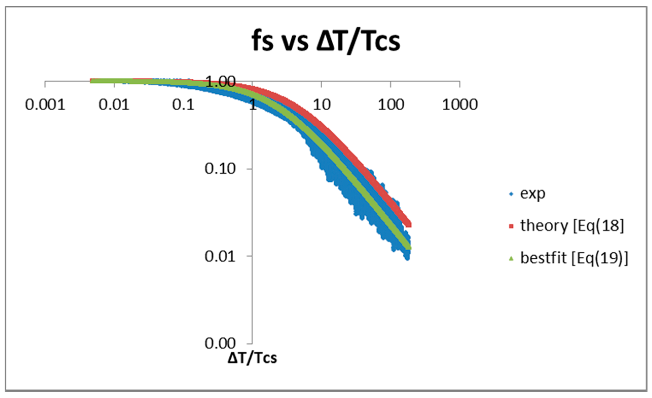
Equation (17) has been integrated numerically and then simple fitting relationships have been attempted to fit the obtained numerical results. It was possible to fit those numerical data with the following relationship:

$$f_S\left(\frac{∆T}{T_{CS}}\right)\approx \frac{1}{1+0.232∆T/{{\rm T}}_{cs}}$$

(18)

To investigate to what degree Equation (18) is realistic, we considered the 1:225-scale wind-tunnel experiment in a semi-idealised urban area (Michelstadt) which is part of the online validation data base CEDVAL-LES (https://mi-pub.cen.uni-hamburg.de/index.php?id=6339). More details for the data and data treatment are given in [52]. Concentration time series from 196 sensors have been generated in that experiment. Each sensor contains 55,000 concentration high time-resolution ($∆{\tau }_0=1.125s$) measurements.

Here, in each sensor time-averaged concentration time series were obtained for time intervals $∆T$ in the range from $\Delta {\tau }_0$ to 1500$∆{\tau }_0$. In total, 196 × 1500 = 294,000 time-averaged concentration time series were produced, and the concentration variance ratios ${\sigma }_{CS}^2/{\sigma }_{CS0}^2$ for each time series were calculated. The results are given in Figure 1 as function of $∆T/T_{CS}$.

In Figure 1 the concentration variance ratio is compared with two curves: one corresponding to the theoretical relationship (18) and one corresponding to the following empirical relationship that seems to fit better the experimental results.

$$f_S\left(\frac{\Delta {\rm T}}{T_{CS}}\right)\approx \frac{1}{1+0.42∆T/T_{CS}}$$

(19)

It is interesting to see that the theoretical curve (18) is not only well correlated with the experimental data, but it is also serving as their upper bound. One explanation could be that in the theory the pollutant is assumed to be well mixed along all turbulent scales, an assumption which is not always true in reality.

It is worth underlying here that the formulation (18) sets the concentration fluctuation statistics as a function of the integration time interval in a completely new basis with solid roots in the theory. The replacement of the fitting parameter 0.232 by the value 0.42 as suggested in Equation (19) was obtained from only the above wind tunnel experiment but with a relatively dense sensor network reflecting a considerable variety of downwind distances, orientations with respect to the wind direction and local geometric characteristics. This gives some validity in the direction of obtaining a value applicable for dispersion in urban environments. Obviously more experimental work including the real atmospheric environment will be needed.

In the remainder we adopt the more realistic Equation (19) to estimate standard deviations in the various time intervals $\Delta {\rm T}$.

3. The Experimental Evidence: The S2 Michelstadt Experiment for Puff and Continuous Releases

As stated above, an important effort here is to seek experimental evidence on the dosage statistics relationships between puff and continuous releases.

The present study is considered as a first attempt to examine to what extent such a hypothesis is realistic and therefore is limited to the S2 Michelstadt Experiment for puff and continuous releases. The selection of this particular experiment is justified by the fact that it is a well-studied experiment and it has been numerically simulated in the past [53,54,55].

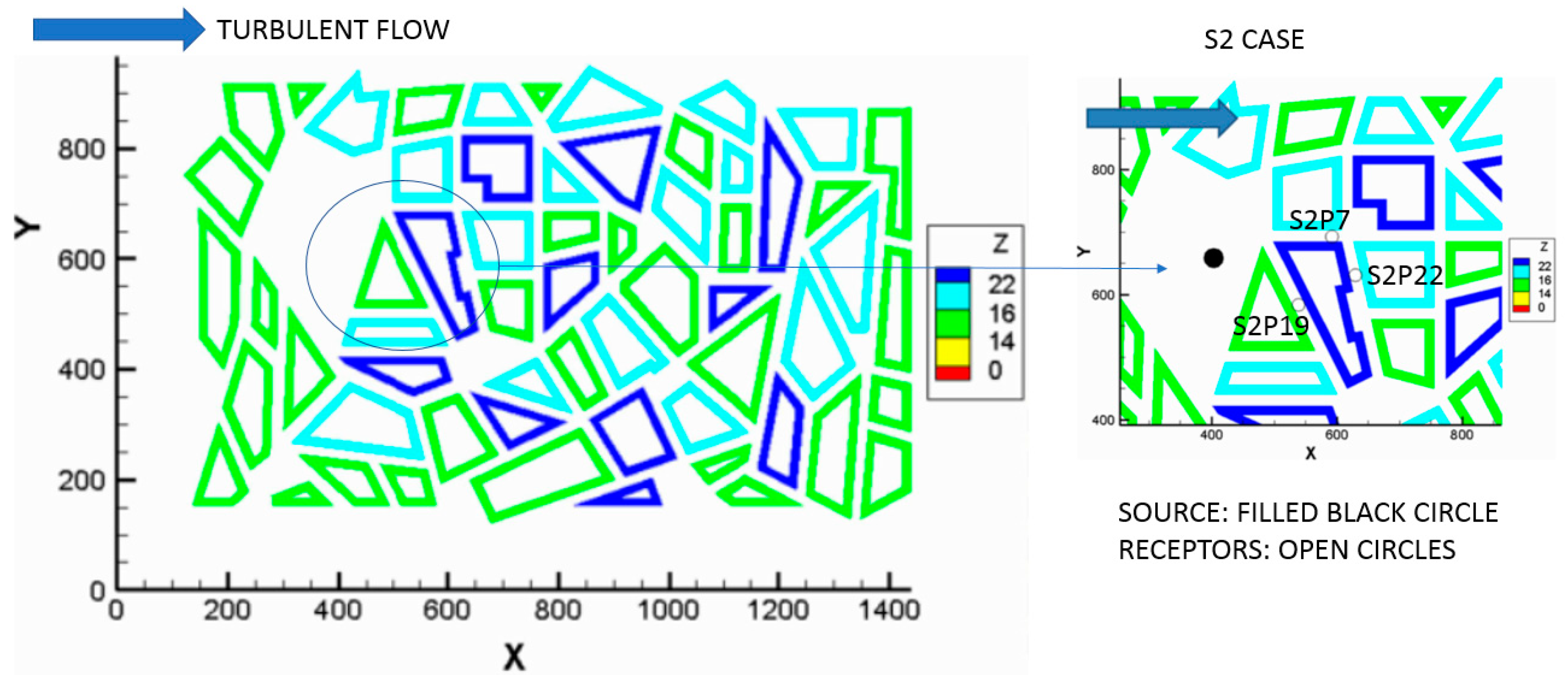
The S2 source is located on the ground in an open space as shown in Figure 2.

The sensors are located at 7.5 m above ground (in real scale). In this study the three sensors shown in Figure 2 were considered which are common for both the puff and continuous releases.

In case of the continuous release the flow rate of the tracer gas was 0.5 kg s⁻¹ while in case of the “instantaneous” (short-duration) release the released quantity per puff was 10 kg and the release duration per puff was 29 s. In total, 286 puffs were released with a time distance between two successive releases of the order of 10 min.

For each puff the experiment produced measurements for several parameters such as dosage, peak concentration and peak concentration based on 15-s average, together with concentration signal time characteristics such as arrival, peak and departure times.

3.1. The Puff Releases vs. the Continuous Release Comparisons

The present puff release experimental data study strengthens the hypotheses that the dosage is the key defining parameter and the peak concentrations can be derived from the dosages not only in terms of ensemble averages and standard deviations but also in terms of pdf/cdf. What is needed on this problem is further scientific evidence to quantify more precisely their respective correlation factors although the $\sigma /m$ (standard deviation over mean) ratio shows a bit more clearly a relationship close to unity.

As mentioned above, the problem in this section is finite-duration release dosage quantification both in terms of ensemble average and standard deviation. We tried to seek experimental evidence for the proposed interrelationship by performing puff releases vs. continuous release comparisons in the abovementioned S2 Michelstadt experiment.

To ensure intercomparison data coherence all 286 experimental puffs were considered including the non-detected puffs at the sensors shown in Figure 2 as well. The undetected puffs were included assigning a zero value for the dosage. The dosage data for the puff releases and the steady-state concentration data for the continuous release at the three sensors are summarised in

Table 1. The S2 Michelstadt experiment: data for the 286 puff releases and the continuous release (for the puff releases $m=\overline{D}/QT$ and $\sigma ={\sigma }_D/QT$; for the continuous release $m=\overline{CS}/Q$, $\sigma ={\sigma }_{CS0}/Q$ and $\sigma \left(29s\right)={\sigma }_{CS}\left(29s\right)/Q$).

Sensors	Puff Releases			Continuous Release
	Non Detected Puffs	Normalised Dosage (ppm s/kg)		Normalised Concentrations (ppm s/kg)			Turbulence Time Scales (s)
		m	σ	m	σ	σ (29 s)(*)
S2P7	31/286	124.73	116.60	125.85	145.06	114.36	19.20
S2P19	44/286	86.42	88.99	32.27	43.44	39.58	59.54
S2P22	4/286	85.49	62.56	78.79	56.20	49.31	40.69

(*) Estimated from Equations (14) and (19).

. It is noted that following the formulation of Equations (5) and (6) the dosage ensemble averages and corresponding standard deviations are normalised by the total puff mass release ($m=\overline{D}/QT$ and $\sigma ={\sigma }_D/QT$), while the steady state concentrations and corresponding standard deviations are normalised by the single puff mass release rate ($m=\overline{CS}/Q$, $\sigma ={\sigma }_{CS0}/Q$ and $\sigma \left(29s\right)={\sigma }_{CS}\left(29s\right)/Q$). In this table, the concentration turbulence time scales as estimated from the continuous concentration signal are included as well.

It can be seen from Table 1 that not all puffs were detected in each sensor. The sensor S2P19 shows the lowest detection ratio indicating a relatively higher degree of unstable flow behaviour.

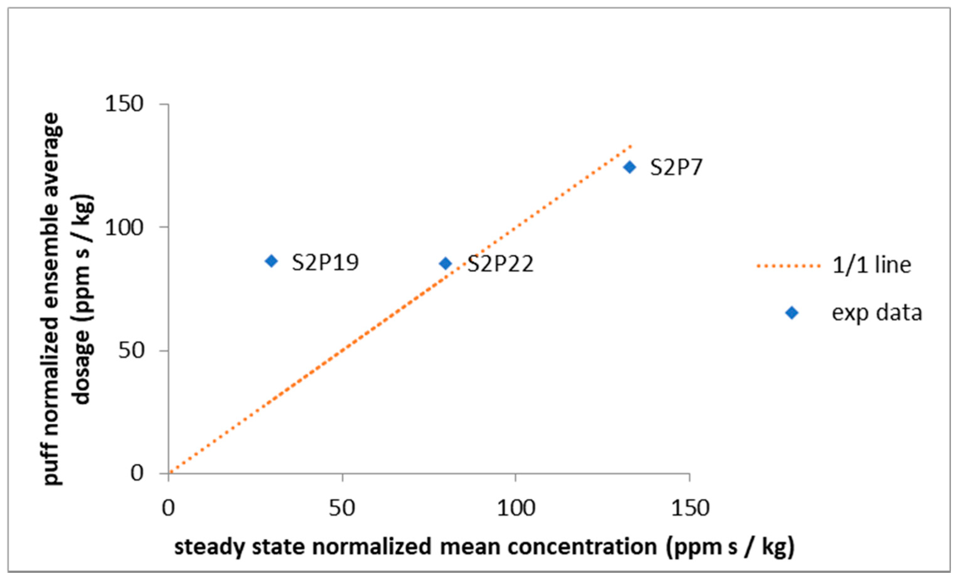
In Figure 3 the puff release normalised ensemble average dosage is compared with the equivalent continuous release steady state normalised concentration to test the validity of Equation (12). The comparison is fairly good with the largest discrepancy in the sensor S2P19. This sensor is associated with the highest number of undetected puffs. Such behaviour is expected to be associated with significant flow unsteadiness [56]. It should be noted that in the present approach the key assumption is that the RANS approximation is valid. Apparently, this assumption in the neighbourhood of the sensor S2P19 is questionable. In fact, there are many studies in the literature revealing the RANS weakness in replicating unsteady flows (e.g., [57,58,59,60,61]).

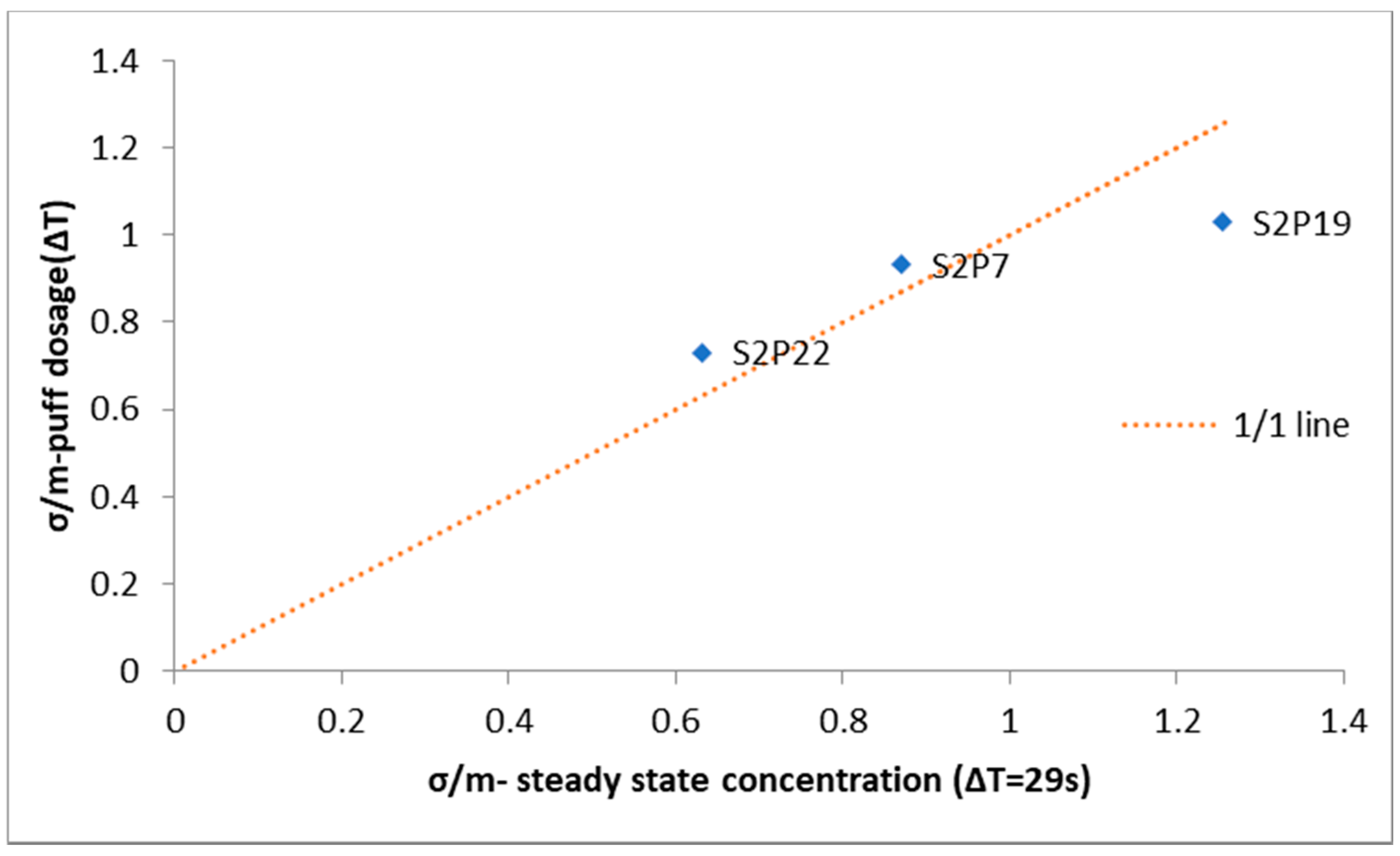
Figure 4 shows the intercomparisons of the $\sigma /m$ ratios for the puff release normalised dosage and the continuous release normalised steady-state concentration. It is noted that for the continuous release the standard deviation $\sigma \left(29s\right)$ of the normalised steady-state concentration is derived by the relationships (14) and (19) using the concentration signal standard deviation (${\sigma }_{CS0}$) and autocorrelation time ($T_{CS}$) and the puff release duration ($∆T=29s$).

It is shown that the correlation between the steady state and the puff releases $\sigma /m$ ratios is quite good and close to unity.

Thus, the present results support the hypotheses as expressed by Equations (5) and (6). The first estimate of the associated coefficients is:

$${\alpha }_m\approx {\alpha }_{\sigma }\approx 1$$

(20)

This is an important finding that strengthens the hypothesis that prediction of puff release dosage statistics can be derived directly from the equivalent continuous release concentration statistics.

3.2. The Puff Release Experiment Peak Concentrations

In case of a finite-duration release, sometimes in exposure studies we are interested not only in the dosage but in the peak concentrations as well. Here it is examined to what degree the peak concentrations are correlated with the corresponding dosages. We focus on the peak concentrations given by the experiment, i.e., the directly measured peak concentrations and the 15-s time-averaged peak concentrations. The data in terms of ensemble averages (m) and standard deviations (σ) normalised by the single puff mass release rate at the three sensors are summarised in

Table 2. The puff releases dosage and peak concentration (m: ensemble average, σ: standard deviation) normalised by the released puff mass and the puff release rate, respectively.

Sensor	Normalised Peak Concentration (ppm·s/kg)		15-s Time-Averaged Normalised Peak Concentration (ppm·s/kg)
	m	σ	m	σ
S2P7	160.00	121.92	88.05	69.26
S2P19	53.66	49.21	29.51	29.08
S2P22	63.80	48.67	36.91	27.15

.

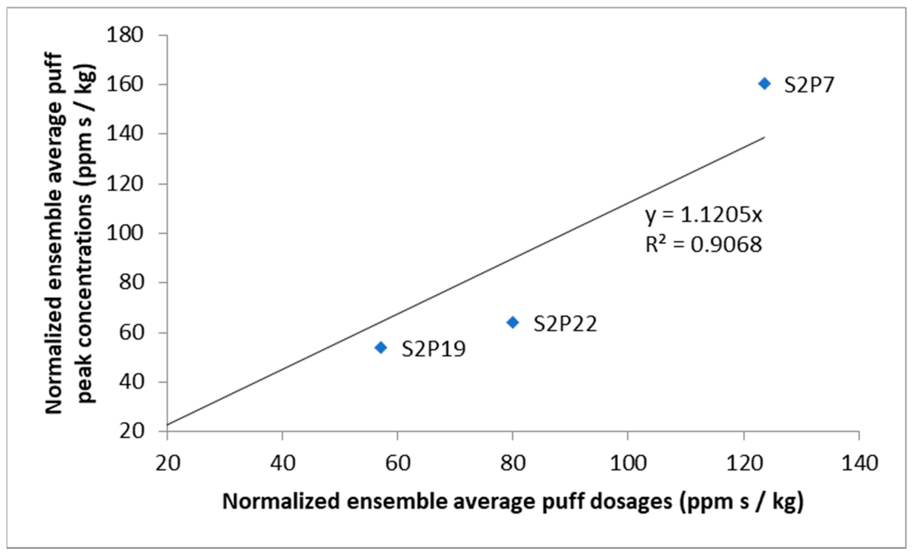
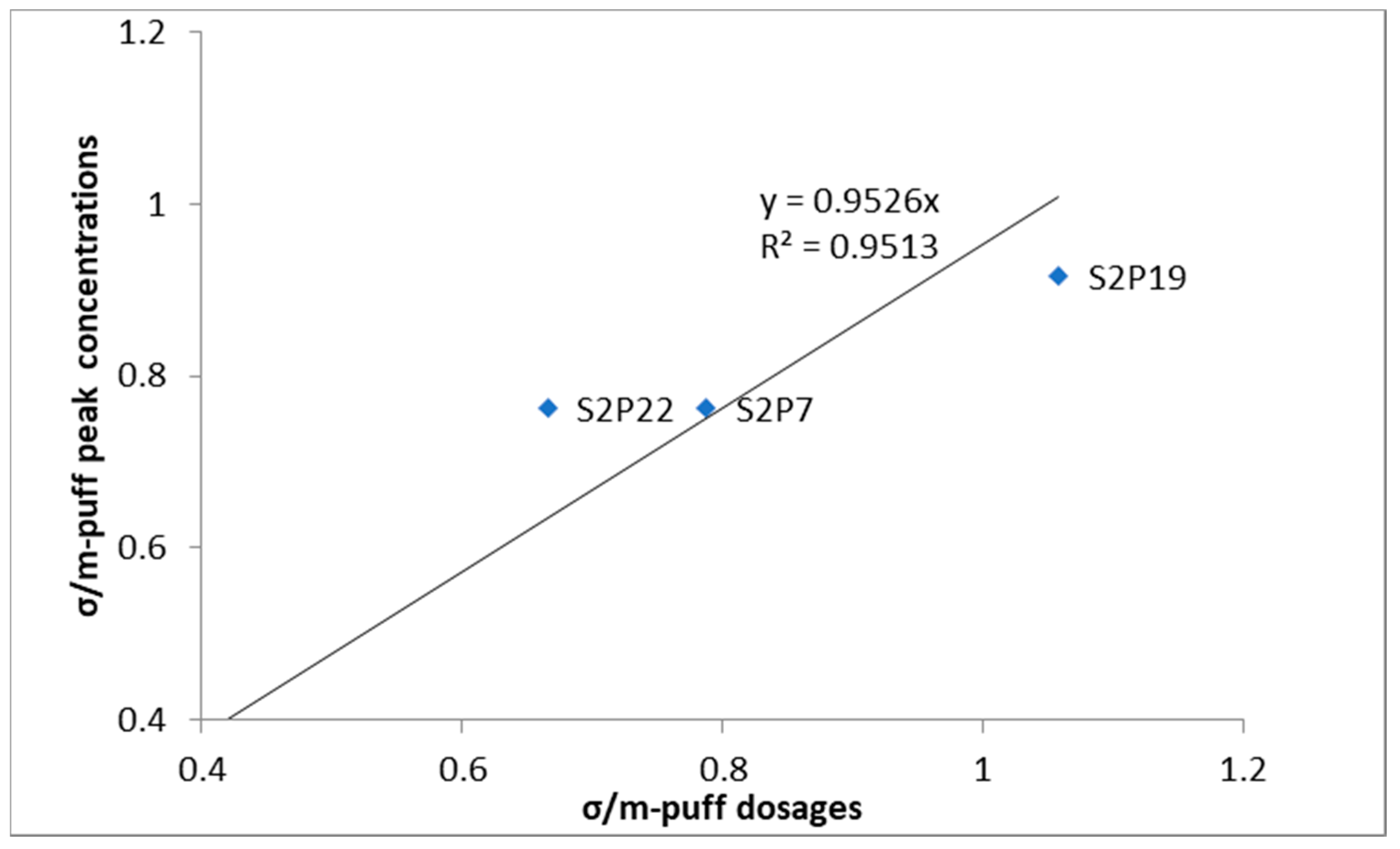
In Figure 5 and Figure 6a a comparison is shown between dosages and peak concentrations in terms of ensemble averages and $\sigma /m$ (standard deviation over ensemble average) ratios at the three sensor locations.

It seems that there is a correlation for both parameters (i.e., m and $\sigma /m$) connecting peak concentration and dosages. The present results indicate a correlation factor in the order of unity. However, further investigations are needed to draw more precise estimations.

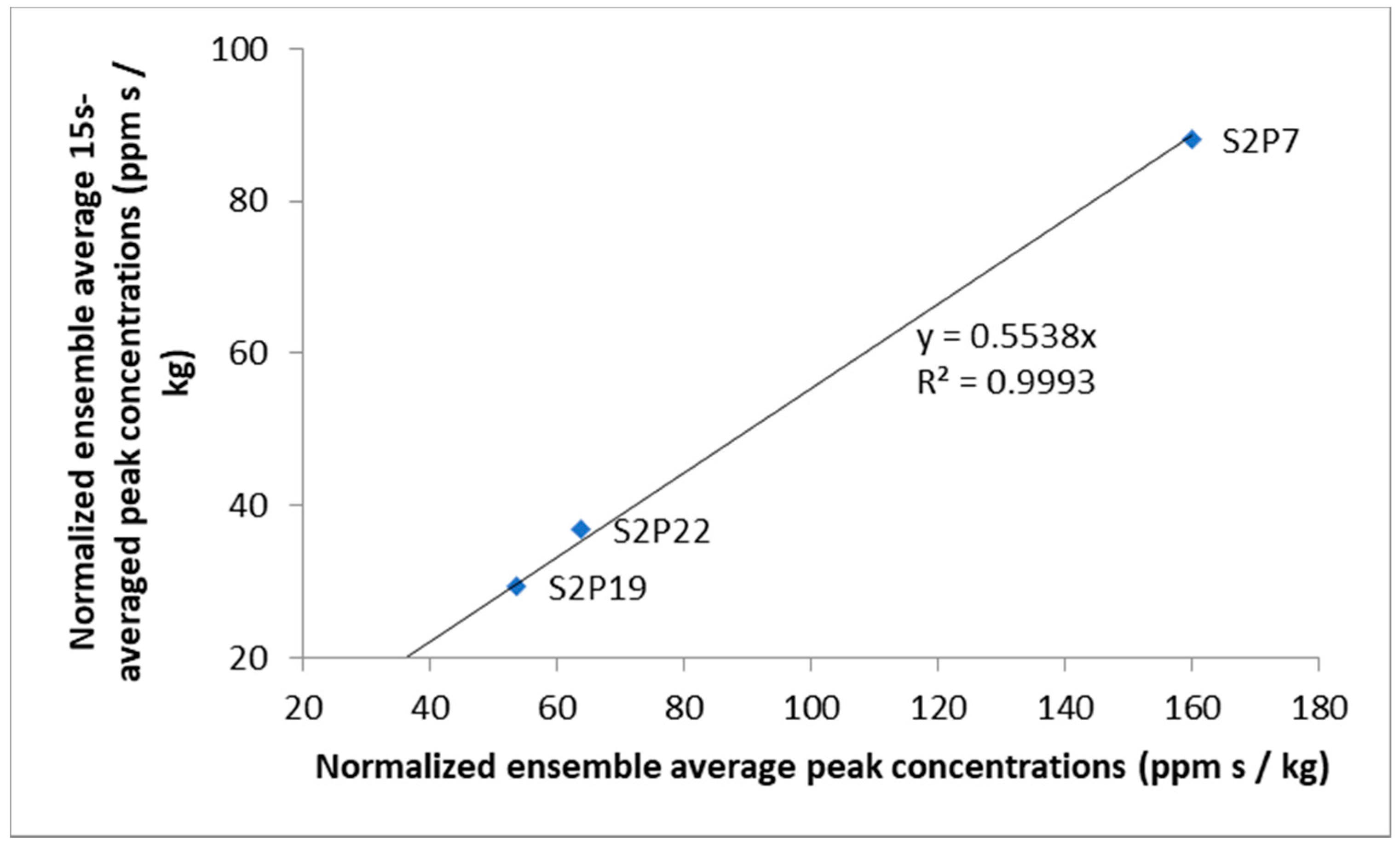
An important question that also needs to be answered is how the concentrations averaged over larger time intervals behave. In Figure 7 we compare the ensemble average peak concentrations with the ensemble average peak concentrations derived from moving concentration averages over 15 s. There is almost a perfect correlation with an estimated factor of 0.554. A lower value than unity was expected due to concentration signal 15-s time filtering. However further experimental evidence is needed before any factor value assessment is attempted.

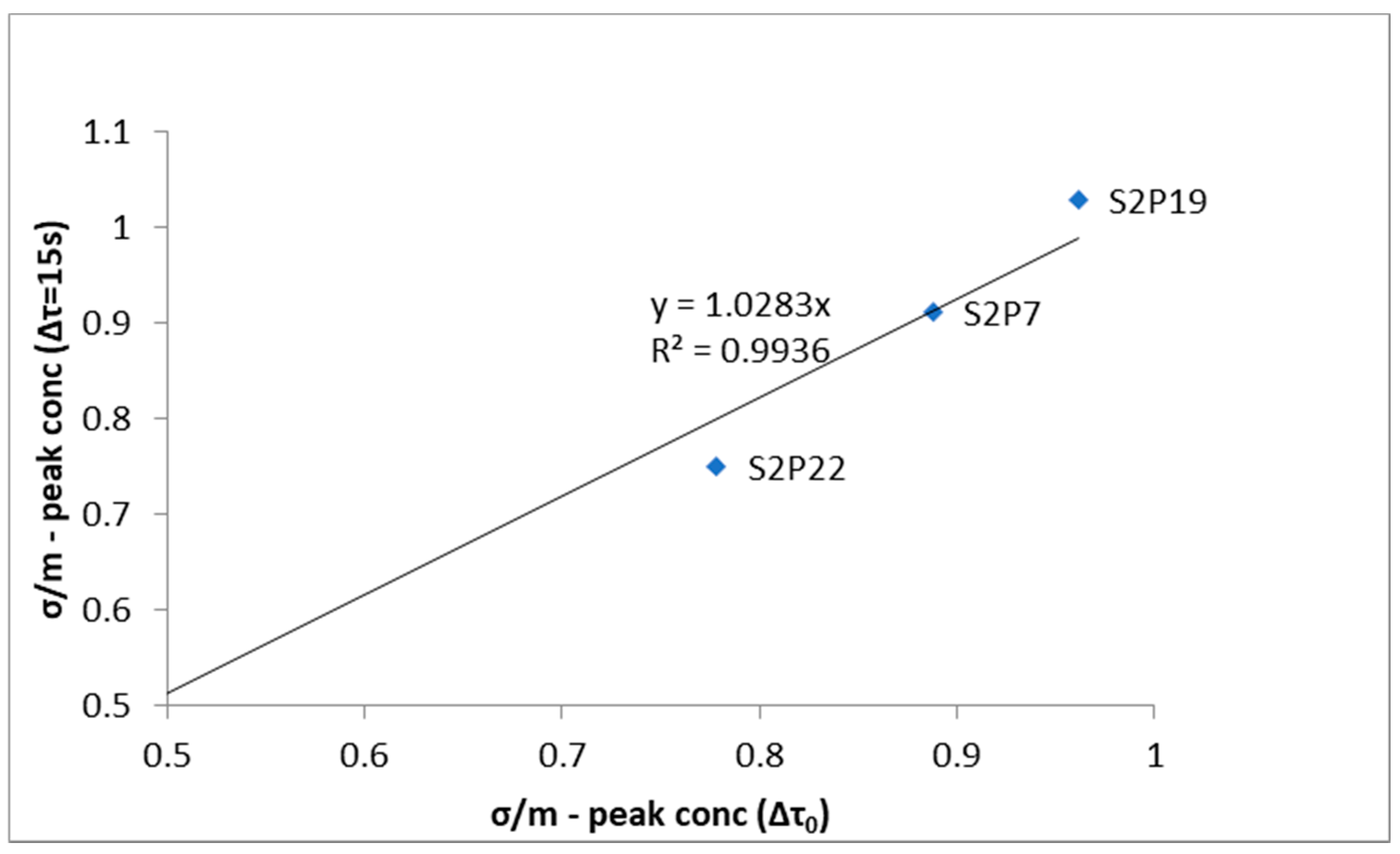
In Figure 8, it is interesting to see that the $\sigma /m$ ratios are also correlated by a factor of unity.

3.3. Dosage/Peak Concentrations Pdf/Cdf for Puff Releases

The continuous release dosage and concentration statistical behaviour in terms of probability density function (pdf)/cumulative density function (cdf) has been extensively discussed in [52]. The beta function seems to be the appropriate generic approximation for the concentration/dosage pdf. Here we will examine to what degree the beta function as applied in [52] is also the proper pdf/cdf approximation for the puff release dosage and peak concentration.

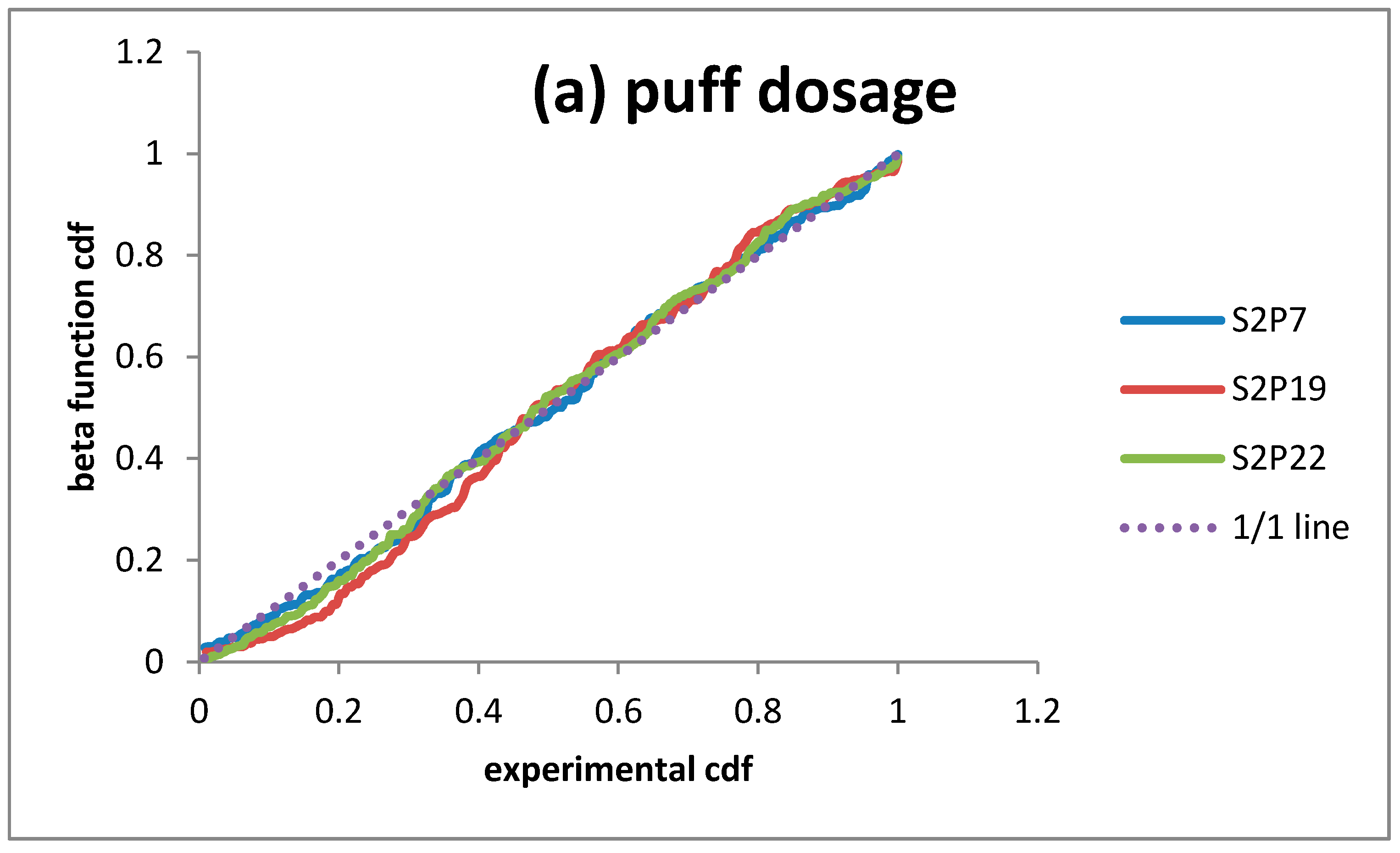
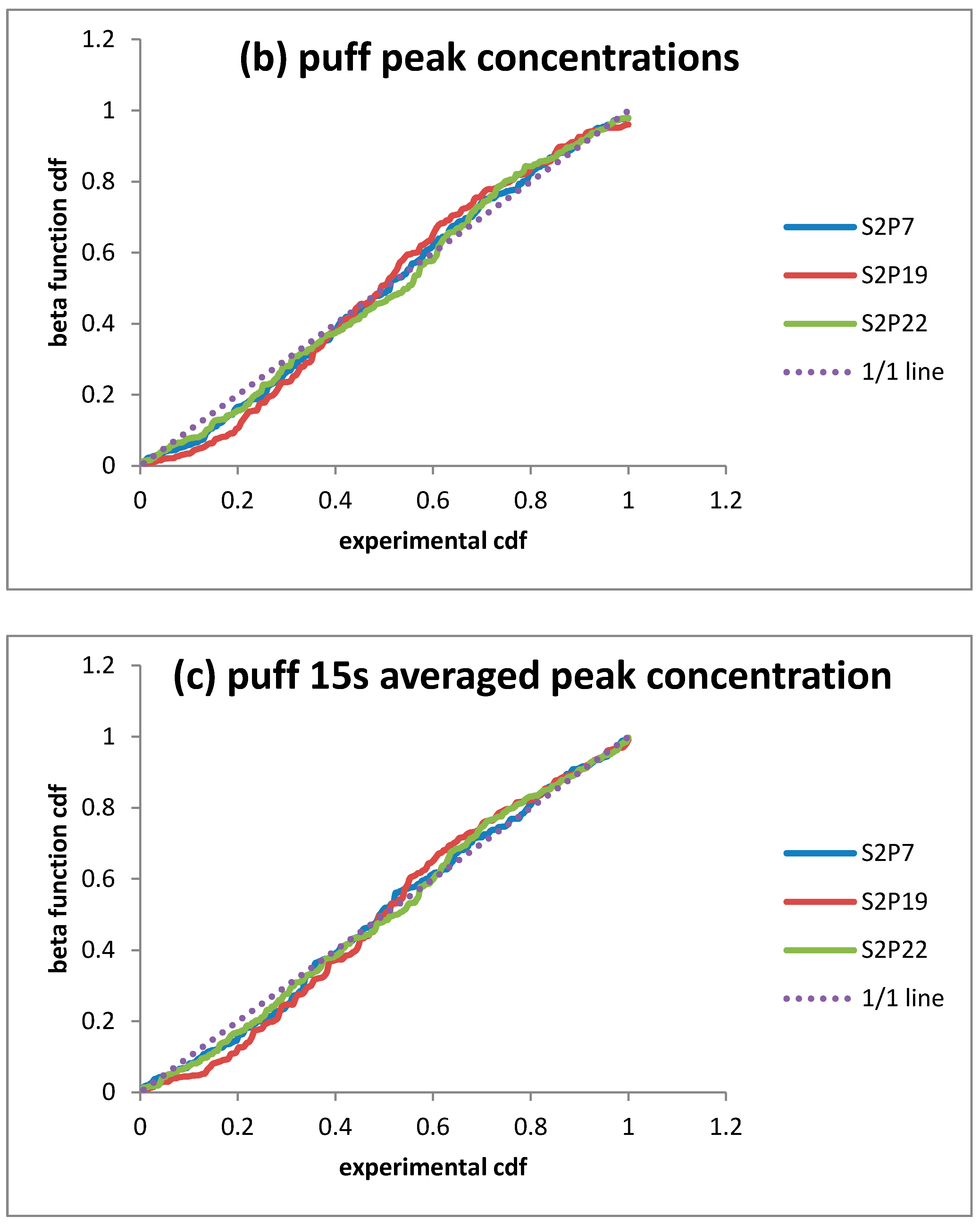
In Figure 9a–c the theoretical (beta function) vs. experimental cdf’s are given for puff dosages and peak concentrations.

It is noted that a perfect fir would follow the 1:1 line. Figure 9 shows that the beta function as introduced in [52] seems to be a good pdf/cdf approximation not only for dosages but for peak concentrations as well. This means that if the ensemble average and standard deviation for those parameters are known or can be predicted, the detailed pdf/cdf can be also adequately approximated.

4. Conclusions

The exposure due to airborne hazardous releases of short time duration is stochastic in nature and strongly dependent on the release duration. Its assessment often requires a relatively large number of dispersion simulations especially if one needs to consider a range of release durations and at the same time reveal the statistical behaviour of the associated exposure parameters due to atmospheric turbulence. The present analysis introduces the novel approach to replace all the above-mentioned simulation scenarios by only one simulation corresponding to a continuous release scenario and derive the exposure parameterisation for each individual scenario by simple relationships.

The present analysis was concentrated on dosages and peak concentrations, the primary parameters in assessing downstream exposures.

Having established the steady-state concentration $\overline{CS}$ of the corresponding continuous release and its standard deviation ${\sigma }_{CS0}^2$ (either from high-time-resolution experimental measurements or from CFD modelling), the dosage ensemble average for short-duration releases is given by Equation (5), its standard deviation is given by Equations (6), (14) and (19), while its pdf/cdf is given by the beta function introduced by [52]. The associated coefficients are given by the Equation (20). All those relationships are as valid as the RANS approximation expressed by Equation (7).

Furthermore, the present experimental data analysis supports the hypothesis that the peak concentration statistics for short-duration releases in terms of ensemble average and standard deviation are well correlated with the corresponding dosage statistics. However, for more reliable quantification of the associated correlation coefficients, further experimental and theoretical research is needed. The pdf/cdf of peak concentration from short-duration releases can also be approximated by the beta function proposed by [52] for continuous releases.

It should be underlined that the whole methodology does not depend on source strength or sensor distances from the source. Although the presented theoretical evidence is rather solid, increasing the degree of confidence and reliability, the presented methodology evaluation is based on rather limited experimental data mainly due to a relatively small number of existing measuring sensors in the wind-tunnel experiments. There is a need for further research especially in expanding the relevant experimental data base.

References

- Andronopoulos, S.; Bartzis, J.G.; Efthimiou, G.C.; Venetsanos, A.G. Puff-dispersion variability assessment through Lagrangian and Eulerian modelling based on the JU2003 campaign. Bound. Layer Meteorol. 2019, 171, 395–422. [Google Scholar] [CrossRef]
- Berbekar, E.; Harms, F.; Leitl, B. Dosage-based parameters for characterization of puff dispersion results. J. Hazard. Mater. 2015, 283, 178–185. [Google Scholar] [CrossRef] [PubMed]
- Hanna, S.; Chang, J.; Mazzola, T. Comparison of an Analytical Urban Puff-Dispersion Model with Tracer Observations from the Joint Urban 2003 Field Campaign. Bound. Layer Meteorol. 2019, 171, 377–393. [Google Scholar] [CrossRef]
- Hernández-Ceballos, M.A.; Hanna, S.; Bianconi, R.; Bellasio, R.; Chang, J.; Mazzola, T.; Andronopoulos, S.; Armand, P.; Benbouta, N.; Čarný, P.; et al. UDINEE: Evaluation of Multiple Models with Data from the JU2003 Puff Releases in Oklahoma City. Part II: Simulation of Puff Parameters. Bound. Layer Meteorol. 2019, 171, 351–376. [Google Scholar] [CrossRef]
- Oldrini, O.; Armand, P. Validation and Sensitivity Study of the PMSS Modelling System for Puff Releases in the Joint Urban 2003 Field Experiment. Bound. Layer Meteorol. 2019, 171, 513–535. [Google Scholar] [CrossRef]
- Trini Castelli, S.; Armand, P.; Tinarelli, G.; Duchenne, C.; Nibart, M. Validation of a Lagrangian particle dispersion model with wind tunnel and field experiments in urban environment. Atmos. Environ. 2018, 193, 273–289. [Google Scholar] [CrossRef]
- Chaloupecká, H.; Jakubcová, M.; Janour, Z.; Jurcáková, K.; Kellnerová, R. Equations of a new puff model for idealized urban canopy. Process Saf. Environ. Prot. 2019, 126, 382–392. [Google Scholar] [CrossRef]
- Hanna, S.R.; Brown, M.J.; Camelli, F.E.; Chan, S.T.; Coirier, W.J.; Hansen, O.R.; Huber, A.H.; Kim, S.; Reynolds, R.M. Detailed simulations of atmospheric flow and dispersion downtown Manhattan: An application of five computational fluid dynamics models. Bull Am. Meteorol. Soc. 2006, 87, 1713–1726. [Google Scholar] [CrossRef] [Green Version]
- Chan, S.T.; Leach, M.J. A validation of FEM3MP with Joint Urban 2003 data. J. Appl. Meteorol. Clim. 2007, 46, 2127–2146. [Google Scholar] [CrossRef] [Green Version]
- Flaherty, J.E.; Stock, D.; Lamb, B. Computational fluid dynamic simulations of plume dispersion in urban Oklahoma City. J. Appl. Meteorol. Clim. 2007, 46, 2110–2126. [Google Scholar] [CrossRef]
- Hendricks, E.A.; Diehl, S.R.; Burrows, D.A.; Keith, R. Evaluation of a fast-running urban dispersion modeling system using Joint Urban 2003 field data. J. Appl. Meteorol. Clim. 2007, 46, 2165–2179. [Google Scholar] [CrossRef]
- Warner, S.; Platt, N.; Urban, J.T.; Heagy, J.F. Comparisons of transport and dispersion model predictions of the Joint Urban 2003 field experiment. J. Appl. Meteorol. Clim. 2008, 47, 1910–1928. [Google Scholar] [CrossRef]
- Hanna, S.R.; White, J.M.; Troiler, J.; Vernot, R.; Brown, M.; Kaplan, H.; Alexander, Y.; Moussafir, J.; Wang, Y.; Williamson, C.; et al. Comparisons of JU2003 observations with four diagnostic urban wind flow and Lagrangian particle dispersion models. Atmos. Environ. 2011, 45, 4073–4081. [Google Scholar] [CrossRef]
- Baumann-Stanzer, K.; Andronopoulos, S.; Armand, P.; Berbekar, E.; Efthimiou, G.; Fuka, V.; Gariazzo, C.; Gasparac, G.; Harms, F.; Hellsten, A.; et al. COST ES1006-Model Evaluation Case Studies: Approach and Results; COST Office: Brussels, Belgium, 2015; ISBN 987-3-9817334-2-6. [Google Scholar]
- Trini Castelli, S.; Tinarelli, G.; Reisin, T.G. Comparison of atmospheric modelling systems simulating the flow, turbulence and dispersion at the microscale within obstacles. Environ. Fluid Mech. 2017, 17, 879–901. [Google Scholar] [CrossRef]
- Chatwin, P.C. The use of statistics in describing and predicting the effects of dispersing gas clouds. J. Hazard. Mater. 1982, 6, 213–230. [Google Scholar] [CrossRef]
- Bogen, K.T.; Gouveia, F.J. Impact of spatiotemporal fluctuations in airborne chemical concentration on toxic hazard assessment. J. Hazard. Mater. 2008, 152, 228–240. [Google Scholar] [CrossRef]
- Mole, N.; Clarke, E.D. Relationships between higher moments of concentration and of dose in turbulent dispersion. Bound. Layer Meteorol. 1995, 73, 35–52. [Google Scholar] [CrossRef]
- Hilderman, T.L.; Hrudey, S.E.; Wilson, D.J. A model for effective toxic load from fluctuating gas concentrations. J. Hazard. Mater. 1999, 64, 115–134. [Google Scholar] [CrossRef]
- Hanna, S.R. The exponential probability density function and concentration fluctuations in smoke plumes. Bound. Layer Meteorol. 1984, 29, 361–375. [Google Scholar] [CrossRef]
- Yee, E. The shape of the probability density function of short-term concentration fluctuations of plumes in the atmospheric boundary layer. Bound. Layer Meteorol. 1990, 51, 269–298. [Google Scholar] [CrossRef]
- Weil, J.C.; Sykes, R.I.; Venkatram, A. Evaluating air-quality models: Review and outlook. J. Appl. Meteorol. 1992, 31, 1121–1145. Available online: http://www.jstor.org/stable/26186554 (accessed on 4 January 2021). [CrossRef] [Green Version]
- Yee, E.; Wilson, D.J.; Zelt, B.W. Probability distributions of concentration fluctuations of a weakly diffusive passive plume in turbulent boundary layer. Bound. Layer Meteorol. 1993, 64, 321–354. [Google Scholar] [CrossRef]
- Yee, E.; Kosteniuk, P.R.; Chandler, G.M.; Biltoft, C.A.; Bowers, J.F. Statistical characteristics of concentration fluctuations in dispersing plumes in the atmospheric surface layer. Bound. Layer Meteorol. 1993, 65, 69–109. [Google Scholar] [CrossRef]
- Lung, T.; Müller, H.-J.; Gläser, M.; Möller, B. Measurements and modelling of full-scale concentration fluctuations. Agratechnische Forsch. 2002, 8, 5–15. [Google Scholar]
- Csanady, G.T. Concentration fluctuations in turbulent diffusion. J. Atmos. Sci. 1967, 24, 21–28. [Google Scholar] [CrossRef] [Green Version]
- Andronopoulos, S.; Grigoriadis, D.; Robins, A.; Venetsanos, A.; Rafailidis, S.; Bartzis, J.G. Three-dimensional modelling of concentration fluctuations in complicated geometry. Environ. Fluid Mech. 2001, 1, 415–440. [Google Scholar] [CrossRef]
- Hsieh, K.-J.; Lien, F.-S.; Yee, E. Numerical modeling of passive scalar dispersion in an urban canopy layer. J. Wind Eng. Ind. Aerodyn. 2007, 95, 1611–1636. [Google Scholar] [CrossRef]
- Mavroidis, I.; Andronopoulos, S.; Bartzis, J.G.; Griffiths, R.F. Atmospheric dispersion in the presence of a three-dimensional cubical obstacle: Modelling of mean concentration and concentration fluctuations. Atmos. Environ. 2007, 41, 2740–2756. [Google Scholar] [CrossRef]
- Milliez, M.; Carissimo, B. Computational Fluid Dynamical Modelling of Concentration Fluctuations in an Idealized Urban Area. Bound. Layer Meteorol. 2008, 127, 241–259. [Google Scholar] [CrossRef]
- Yee, E.; Wang, B.-C.; Lien, F.-S. Probabilistic Model for Concentration Fluctuations in Compact-Source Plumes in an Urban Environment. Bound. Layer Meteorol. 2009, 130, 169–208. [Google Scholar] [CrossRef]
- Leuzzi, G.; Amicarelli, A.; Monti, P.; Thomson, D.J. A 3D Lagrangian micromixing dispersion model LAGFLUM and its validation with a wind tunnel experiment. Atmos. Environ. 2012, 54, 117–126. [Google Scholar] [CrossRef]
- Dourado, H.; Santos, J.M.; Reis, N.C., Jr.; Mavroidis, I. Development of a fluctuating plume model for odour dispersion around buildings. Atmos. Environ. 2014, 89, 148–157. [Google Scholar] [CrossRef]
- Manor, A. A Stochastic Single-Particle Lagrangian Model for the Concentration Fluctuations in a Plume Dispersing Inside an Urban Canopy. Bound. Layer Meteorol. 2014, 150, 327–340. [Google Scholar] [CrossRef]
- Mavroidis, I.; Andronopoulos, S.; Venetsanos, A.; Bartzis, J.G. Numerical investigation of concentrations and concentration fluctuations around isolated obstacles of different shapes. Comparison with wind tunnel results. Environ. Fluid Mech. 2015, 15, 999–1034. [Google Scholar] [CrossRef]
- Efthimiou, G.C.; Berbekar, E.; Harms, F.; Bartzis, J.G.; Leitl, B. Prediction of high concentrations and concentration distribution of a continuous point source release in a semi-idealized urban canopy using CFD-RANS modeling. Atmos. Environ. 2015, 100, 48–56. [Google Scholar] [CrossRef]
- Efthimiou, G.C.; Andronopoulos, S.; Tolias, I.; Venetsanos, A. Prediction of the upper tail of concentration distributions of a continuous point source release in urban environments. Environ. Fluid Mech. 2016, 16, 899–921. [Google Scholar] [CrossRef]
- Efthimiou, G.C.; Andronopoulos, S.; Bartzis, J.G. Evaluation of probability distributions for concentration fluctuations in a building array. Physica A 2017, 484, 104–116. [Google Scholar] [CrossRef]
- Efthimiou, G.C. Prediction of four concentration moments of an airborne material released from a point source in an urban environment. J. Wind Eng. Ind. Aerodyn. 2019, 184, 247–255. [Google Scholar] [CrossRef]
- Davidson, M.J.; Snyder, W.H.; Lawson, R.E., Jr.; Hunt, J.C.R. Wind tunnel simulations of plume dispersion through groups of obstacles. Atmos. Environ. 1996, 30, 3715–3731. [Google Scholar] [CrossRef]
- Pavageau, M.; Schatzmann, M. Wind tunnel measurements of concentration fluctuations in an urban street canyon. Atmos. Environ. 1999, 33, 3961–3971. [Google Scholar] [CrossRef]
- Yee, E.; Biltoft, C.A. Concentration fluctuation measurements in a plume dispersing through a regular array of obstacles. Bound. Layer Meteorol. 2004, 111, 363–415. [Google Scholar] [CrossRef]
- Santos, J.M.; Griffiths, R.F.; Roberts, I.D.; Reis, N.C., Jr. A field experiment on turbulent concentration fluctuations of an atmospheric tracer gas in the vicinity of a complex-shaped building. Atmos. Environ. 2005, 39, 4999–5012. [Google Scholar] [CrossRef]
- Gailis, R.M.; Hill, A. A wind-tunnel simulation of plume dispersion within a large array of obstacles. Bound. Layer Meteorol. 2006, 119, 289–338. [Google Scholar] [CrossRef]
- Yee, E.; Chan, R.; Kosteniuk, P.R.; Chandler, G.M.; Biltoft, C.A.; Bowers, J.F. Concentration fluctuation measurements in clouds released from a quasi-instantaneous point source in the atmospheric surface layer. Bound. Layer Meteorol. 1994, 71, 341–373. [Google Scholar] [CrossRef]
- Yee, E.; Kosteniuk, P.R.; Bowers, J.F. Study of concentration fluctuations in instantaneous clouds dispersing in the atmospheric surface layer for relative turbulent diffusion: Basic descriptive statistics. Bound. Layer Meteorol. 1998, 87, 409–457. [Google Scholar] [CrossRef]
- Cassiani, M.; Bertagni, M.B.; Marro, M.; Salizzoni, P. Concentration fluctuations from localized atmospheric releases. Bound. Layer Meteorol. 2020, 177, 461–510. [Google Scholar] [CrossRef] [PubMed]
- Andronopoulos, S.; Bartzis, J.G.; Würtz, J.; Asimakopoulos, D. Modelling the effects of obstacles on the dispersion of denser-than-air gases. J. Hazard. Mater. 1994, 37, 327–352. [Google Scholar] [CrossRef]
- Venkatram, A. The expected deviation of observed concentrations from predicted ensemble means. Atmos. Environ. 1979, 13, 1547–1549. [Google Scholar] [CrossRef]
- Park, C.W.; Lee, S.J. The effects of bottom gap and non-uniform porosity in a wind fence on the surface pressure of a triangular prism located behind the fence. J. Wind Eng. Ind. Aerodyn. 2001, 89, 1137–1154. [Google Scholar] [CrossRef]
- Efthimiou, G.C.; Bartzis, J.G. Atmospheric dispersion and individual exposure of hazardous materials. J. Hazard. Mater. 2011, 188, 375–383. [Google Scholar] [CrossRef]
- Bartzis, J.G.; Efthimiou, G.C.; Andronopoulos, S. Modelling Short Term Individual Exposure from Airborne Hazardous Releases in Urban Environments. J. Hazard. Mater. 2015, 300, 182–188. [Google Scholar] [CrossRef] [PubMed]
- Efthimiou, G.C.; Kovalets, I.V.; Argyropoulos, C.D.; Venetsanos, A.; Andronopoulos, S.; Kakosimos, K. Evaluation of an inverse modelling methodology for the prediction of a stationary point pollutant source in complex urban environments. Build. Environ. 2018, 143, 107–119. [Google Scholar] [CrossRef]
- Efthimiou, G.C.; Andronopoulos, S.; Bartzis, J.G. Prediction of dosage-based parameters from the short-duration release of airborne materials in urban environments. Meteorol. Atmos. Phys. 2018, 130, 107–124. [Google Scholar] [CrossRef]
- Rakai, A.; Franke, J. Validation of two RANS solvers with flow data of the flat roof Michelstadt case. Urban Clim. 2014, 10, 758–768. [Google Scholar] [CrossRef]
- Meroney, R.N.; Leitl, B.M.; Rafailidis, S.; Schatzmann, M. Wind-tunnel and numerical modeling of flow and dispersion about several building shapes. J. Wind Eng. Ind. Aerodyn. 1999, 81, 333–345. [Google Scholar] [CrossRef]
- Dagnew, A.K.; Bitsuamlak, G.T. Computational evaluation of wind loads on buildings: A review. Wind Struct. Int. J. 2013, 16, 629–660. [Google Scholar] [CrossRef]
- Hertwig, D.; Efthimiou, G.C.; Bartzis, J.G.; Leitl, B. CFD-RANS model validation of turbulent flow in a semiidealized urban canopy. J. Wind Eng. Ind. Aerodyn. 2012, 111, 61–72. [Google Scholar] [CrossRef]
- Tominaga, Y.; Stathopoulos, T. Numerical simulation of dispersion around an isolated cubic building: Model evaluation of RANS and LES. Build. Environ. 2010, 45, 2231–2239. [Google Scholar] [CrossRef] [Green Version]
- Tominaga, Y.; Mochida, A.; Murakami, S.; Sawaki, S. Comparison of various revised k-ε models and LES applied to flow around a high-rise building model with 1:1:2 shape placed within the surface boundary layer. J. Wind Eng. Ind. Aerodyn. 2008, 96, 389–411. [Google Scholar] [CrossRef]
- Wright, N.G.; Easom, G.J. Non-linear k-ε turbulence model results for flow over a building at full-scale. Appl. Math. Model. 2003, 27, 1013–1033. [Google Scholar] [CrossRef]
Figure 1.
The concentration variance ratio as a function of compared with analytic functions .
Figure 2.
Top view of the buildings configuration in the Michelstadt wind-tunnel experiment (left); source and receptors locations for the S2 Michelstadt puff experiment (right).
Figure 3.
Puff release normalised ensemble average dosage vs. continuous release normalised mean steady state concentration: ensemble averages and means as expressed in Equation (12).
Figure 4.
Puff release vs. continuous release intercomparisons: ratios
Figure 5.
Puff releases: ensemble average (m) values of peak concentrations vs. dosages.
Figure 6.
Puff releases: ratios of peak concentrations vs. dosages.
Figure 7.
Puff releases: ensemble average () values of time-averaged () peak concentrations vs. measured peak concentrations ().
Figure 8.
Puff releases: ratio of time-averaged () peak concentration vs. ratio of measured peak concentrations ().
Figure 9.
Puff releases: Beta function vs. experimental cumulative density function (cdf) for (a) dosage, (b) peak concentrations and (c) 15-s time-averaged peak concentrations.