
Abstract
In the past years weakly deformed optical microdisks have become a focus for fundamental and applied research with lots of interesting new findings. A commonly used method to study such cavities is a perturbation theory based on weak boundary deformations (Dubertrand et al 2008 Phys. Rev. A 77, 013 804). In this paper we extent the perturbation theory to the third order which allows us to improve its accuracy significantly. We discuss various example systems in regard of Q-spoiling, frequency splitting, and far-field emission pattern. The results from the perturbation theory are in a very good agreement to full numerical simulations.
Export citation and abstract BibTeX RIS

Original content from this work may be used under the terms of the Creative Commons Attribution 4.0 licence. Any further distribution of this work must maintain attribution to the author(s) and the title of the work, journal citation and DOI.
1. Introduction
In dielectric whispering-gallery cavities light can be confined for long times via total internal reflection [1]. An often studied type of such whispering-gallery cavities are microdisks which can be effectively described in two dimensions [2–7]. For the purpose of a desired application such microdisks are not perfect circular but rather possess a deformed boundary curve, e.g., to achieve directional light emission from a microlaser [8–16], improve the broadband coupling to an attached waveguide [17], or introduce non-Hermitian degeneracies [18] and wave chaos [9, 10, 19]. It is remarkable that many of the applications like directional emission [20–23], active emission control [24], or the formation of exceptional points [25] can already be realized with very small deformations. On the other hand, slight unintended deformations occur naturally via fabrication tolerances and surface roughness [26–28]. These deformations often have a negative impact on the cavity's performance as they significantly spoil the Q factor [29–31]. Therefore, an efficient treatment of slightly deformed cavities is of large practical and academic interest. Beside a full numerical descriptions, e.g. via the boundary element method (BEM) [32], a second-order perturbation theory for slightly deformed microdisks has been developed in [33]. In its original version the perturbation theory describes transverse-magnetic (TM) polarized modes in a microdisk with a mirror-reflection symmetry. However, generalizations to either transverse-electric (TE) polarized modes [22, 34] or fully asymmetric boundary shapes [35] can be found in the literature. In the past years the perturbation has lead to interesting new findings such as exceptional points in extremely weakly deformed cavities [25, 36] including high-order exceptional points [37], an analytical and transparent descriptions of cavities with sidewall-roughness [38], and the formulation of an inverse problem for far-field optimization [39].
The aim of this article is to extent the perturbation theory to the third order which allows for an improved prediction for TM polarized modes in cavities with a mirror-reflection symmetry. This is advantageous because even numerically exact methods like the BEM have a large effort for extremely weak deformations, e.g., to capture the large Q-factor accurately. Especially in such a case the perturbation theory provides accurate, easy to access, and fast to calculate results.
The paper is organized as follows. In section 2 the mode equation and its solutions for the circular cavity as the unperturbed system are summarized. The perturbation theory for slightly deformed cavities is discussed in section 3 including a brief review of the correction up to the second order and a derivation of the third-order corrections. In section 4 the derived third-order corrections are verified for various example systems. A summary is given in section 5.
2. Mode equation and modes in the circular cavity
Optical microdisk cavities can be treated within a quasi-two-dimensional approximation. In this case Maxwell's equations reduce to a scalar mode equation [40]

for ψ representing either the z-component of the electric field (TM polarization) as  or the magnetic field (TE polarization) as
  . A finite height of the cavity is incorporated here by n being the effective refractive index which is assumed to be homogeneous inside the cavity and unity outside. At the cavity's interface ψ and depending on the polarization the normal derivative ∂ν
ψ (for TM polarization) or the scaled normal derivative n−2∂ν
ψ (for TE polarization) are continuous. In the perturbation theory it is helpful to rescale the complex wavenumber k to the dimensionless frequency x ≡ kR = ω R/c; R is the radius of the disk and c is the speed of light in vacuum. Thus, the quality factor of a mode is given by
. A finite height of the cavity is incorporated here by n being the effective refractive index which is assumed to be homogeneous inside the cavity and unity outside. At the cavity's interface ψ and depending on the polarization the normal derivative ∂ν
ψ (for TM polarization) or the scaled normal derivative n−2∂ν
ψ (for TE polarization) are continuous. In the perturbation theory it is helpful to rescale the complex wavenumber k to the dimensionless frequency x ≡ kR = ω R/c; R is the radius of the disk and c is the speed of light in vacuum. Thus, the quality factor of a mode is given by  . In case of TM polarized fields the complex frequencies in the circular cavity can be calculated as the roots of the function

Here, Jm
and Hm
are the Bessel and Hankel functions of the first kind and order m. A prime ( ) marks the derivative with respect to the argument. The wave function ψ is required to fulfill Sommerfeld's radiation condition. Therefore, the solutions of the mode equation for the circular cavity are

in the interior with r ≤ R and

in the free space for r > R. The angular dependency is given by χ±,m
(ϕ) which we chose as a standing wave, i.e. modes with even parity are expressed as  and modes with odd parity are given by
  with m = 0, 1, 2, ... being the azimuthal mode number. Note that modes with even and odd parity are orthogonal. For m ≠ 0 the solutions for the circular cavity are doubly degenerated. Modes with same azimuthal mode number m but different frequency x can be labeled according to the number of radial intensity maxima inside the cavity with the radial mode number l = 1, 2, 3, .... Note that beside the well confined modes with high quality factors there exist so-called external modes localizing outside of the cavity and having very small quality factors [33, 41, 42]. However, these external modes are omitted in the following.
3. Perturbation theory for weakly deformed microdisks
3.1. General setup and corrections up to the second order
In this section we explain the general setup of the perturbation theory for weakly deformed microdisks with a mirror-reflection symmetry and TM polarized fields. Furthermore, we summarize the known results of the first- and second-order corrections. The detailed derivation of these corrections can be found in [33].
In the perturbation theory the cavity's boundary is expressed in polar coordinates as

where λ is a formally small deformation parameter and f(ϕ) is the deformation function. In contrast to the case of the circular cavity the boundary conditions here explicitly depend on the polar angle ϕ as [ψ±,in − ψ±,out ](r(ϕ), ϕ) = 0 and ∂r [ψ±,in − ψ±,out ](r(ϕ), ϕ) = 0 for TM polarization. Using a Taylor series of these boundary conditions in λ yields


Both equations need to be evaluated in the orders of λ to derive the perturbation theory corrections. To do so, the wave function is expressed with the ansatz


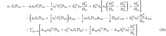
where the (dimensionless) frequency x of the mode in the deformed cavity is the quantity of interest (k = x/R) as well as the coefficients ap and bp . These quantities are again expanded in a series of the perturbation parameter λ up to the third order as
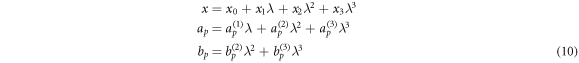
where x0 is the frequency of the considered (unperturbed) mode in the circular cavity with Sm (x0) = 0. Putting both, the expansion (10) and the ansatz (8)–(9), into equations (6)–(7) and comparing the coefficients in order λ1 provides the first-order corrections


Here, Sp = Sp (x0) is shorten and Amp are the Fourier harmonics of the deformation function

with εp = 2 (εp = 1) for p ≠ 0 (p = 0).
In the same way the second-order corrections are derived by evaluating equations (6)–(7) with the ansatz (8)–(9) and the expansion (10) and comparing the coefficients of the order λ2. With the second-order Fourier harmonics of the deformation function

the second-order corrections read


Again the functions are evaluated at x0.
In general, the perturbation theory is expected to give accurate results for sufficiently small λ. In [33] the range of λ has been estimated based on the area where the refractive index is changed via the deformation. However, even if this criterion is violated the perturbation theory can give reasonable results [43]. Contrary, pairs of quasi-degenerate modes within a symmetry class may spoil the accuracy of the perturbation theory which then needs to be adapted [33]. However, this specific case is omitted in the following.
3.2. Derivation of the third-order corrections
In this section the third-order corrections for the perturbation series are derived. To do so, the mode ansatz (8)–(9) and the expansion scheme (10) are used to expand the boundary conditions (6)–(7). Thus, the coefficients of the order λ3 can be compared. In order to simplify these calculations we first define the auxiliary function

where [l] denotes the l-th derivative with respect to the argument. Then, we express the final results with the help of this auxiliary function and its derivatives evaluated at the unperturbed frequency x0; i.e. the third-order corrections are expressed with  and
and  . The derivatives of
  are independent of the deformation and can be calculated explicitly with common computer algebra systems. However, these explicit lengthy expressions are omitted here.
With the help of the auxiliary function  we can write

Here,  is evaluated at the frequency x given from the scheme (10). Hence,
  needs to be expanded as

Inserting this expansion into equation (20) allows to write the boundary conditions (6) and (7) in a series of λ. Comparing the coefficients of the terms λ3 reads
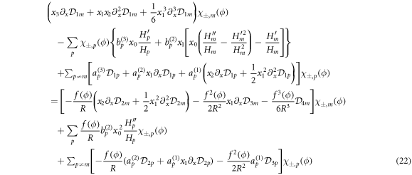
and
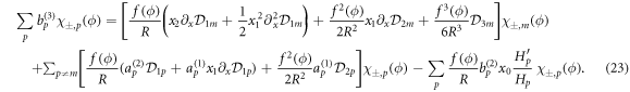
In order to solve this set of equations for the third-order corrections we introduce the third Fourier Harmonics of the deformation

Using orthogonality of the χq (ϕ) we get from equations (22) and (23) the third-order corrections as
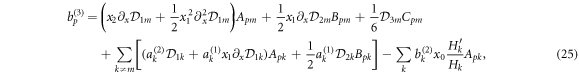
and
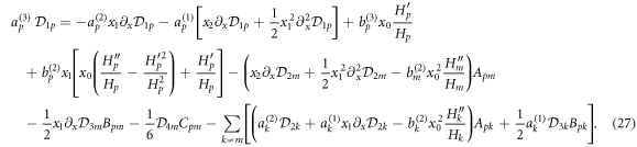
Note that the third-order corrections are written in terms of the first- and second-order corrections which can be found in section 3.1.
4. Application to example systems
In this section we apply the perturbation theory to various example systems. This validates our calculations and illustrates in which cases the third-order corrections lead to a significant improvement of the prediction. The systems studied in the following are shown in figure 1.

Figure 1. Solid curves represent the boundary of the deformed cavities. (a) A shrunken circular cavity with  = 0.2, (b) a quadrupole cavity with = 0.1, (c) a notched circular cavity with (, σ) = (0.1, 0.1), and (d) a shifted limacon cavity with = 0.43. The area where the refractive index is changed via the deformation is colored. The unperturbed circular cavity is shown as dashed curve.
Download figure:
Standard image High-resolution image4.1. Shrunken circular cavity
First, we validate our calculations via a proof of principle. Therefore, the perturbation theory is applied to a circular cavity with a diminished radius (see figure 1(a)). Such a shrunken circular cavity is described within the perturbation theory by the radius in polar coordinates as

Here, the deformation parameter 0 < < 1 directly corresponds to the perturbation parameter λ for a deformation function f(ϕ) = −R in equation (5).
On the other hand, the exact frequencies x analyt in the shrunken circular cavity can be calculated analytically by rescaling the frequencies of the unperturbed circular cavity as

Within this expansion of the exact frequencies the perturbation theory in first (second) [third] order is expected to capture the terms proportional to (2) [3]. Thus, the error of the perturbation theory Err
x = ∣x
analyt
− x
PT
∣ scales with 2 (3) [4] for ≪ 1. This scaling is verified in figure 2 for a mode (m, l) = (16, 1) in a cavity with refractive index n = 2.0. Here, the third-order corrections indeed provide a significant improvement of the perturbation theory. However, it should be kept in mind that the deformation does not lead to a coupling of modes with different azimuthal mode numbers and is therefore very special. Generic examples are discussed below.

Figure 2. The error Err
x of the perturbation theory for the (dash-dotted black curve) first-, (dotted red curve) second- and (solid blue curve) third-order applied to a shrunken circular cavity. The scaling with 2, 3, and 4 is illustrated by dashed lines on the double logarithmic scale.
Download figure:
Standard image High-resolution image4.2. Quadrupolar cavities
A common example for a deformed cavity is the quadrupole which has been studied frequently in terms of ray-wave correspondence, dynamical tunneling and frequency splittings [9, 10, 44–46]. The boundary is given by the radius in polar coordinates as

where is a dimensionless deformation parameter which can be identified directly with the perturbation parameter λ for the deformation function  . In order to grade the perturbation theory the numerical reference value for the error Err
x = ∣x
BEM
− x
PT
∣ of the frequency is calculated with the BEM. As shown in figure 3(a) for the mode with even parity and azimuthal mode number m = 3 in a quadrupole cavity with refractive index n = 1.5 the expected error scaling of the perturbation theory can be observed. In particular, the error of the second order scales with 3 and the error of the third-order scales with 4 until the overall error saturates for small due to the numerical tolerances in the BEM. For modes m > 3, however, the third-order corrections vanish and already the second-order corrections scale with 4 as shown exemplary for the mode (m, l) = (12, 1) in figure 3(b). The reason here is that in regard of the perturbation theory the quadrupole is a rather non-generic deformation due to the single cosine term in f(ϕ) which allows only for specific non-vanishing coupling coefficients in equations (13)–(14), (24). Therefore, Apm
, Bpm
, and Cpm
are rather sparse band matrices leading to the vanishing of the third-order corrections for m > 3.
. In order to grade the perturbation theory the numerical reference value for the error Err
x = ∣x
BEM
− x
PT
∣ of the frequency is calculated with the BEM. As shown in figure 3(a) for the mode with even parity and azimuthal mode number m = 3 in a quadrupole cavity with refractive index n = 1.5 the expected error scaling of the perturbation theory can be observed. In particular, the error of the second order scales with 3 and the error of the third-order scales with 4 until the overall error saturates for small due to the numerical tolerances in the BEM. For modes m > 3, however, the third-order corrections vanish and already the second-order corrections scale with 4 as shown exemplary for the mode (m, l) = (12, 1) in figure 3(b). The reason here is that in regard of the perturbation theory the quadrupole is a rather non-generic deformation due to the single cosine term in f(ϕ) which allows only for specific non-vanishing coupling coefficients in equations (13)–(14), (24). Therefore, Apm
, Bpm
, and Cpm
are rather sparse band matrices leading to the vanishing of the third-order corrections for m > 3.

Figure 3. The error of the first- (second-) [third-] order perturbation theory is shown as dash-dotted black (dotted red) [solid blue] curve for a mode (a) (m, l) = (3, 1) and (b) (m, l) = (12, 1) in a quadrupole cavity, see equation (30). The refractive index is n = 1.5. Dashed gray lines serve as a guide to the eye and indicate the scaling with 2, 3, and 4.
Download figure:
Standard image High-resolution imageIn order to avoid these non-generic behavior of the coupling coefficient Apm , Bpm , and Cpm the cavity's boundary can be slightly modified to the so-called flatten quadrupole [10] defined by

For small ∣∣ ≪ 1 the shape of the quadrupole and the flatten quadrupole cannot be distinguished by eye. However, due to the square root in equation (31) the flatten quadrupole exhibits more coupling terms between modes with different azimuthal mode numbers. Consequently, the third-order corrections are finite and lead to an improvement of the perturbation theory as shown in figure 4(a) for the mode (m, l) = (30, 1). Even though the improvement does not lead to a better scaling with the deformation parameter it yet can be advantageous, e.g., for the prediction of the mode coupling and Q-spoiling due to resonance-assisted tunneling [31, 47]. This can be seen in figure 4(b) where for the flatten quadrupole with = 0.07 the complex frequencies of modes with l = 1 and different azimuthal mode numbers m are shown. The third-order perturbation theory describes the peak in the imaginary part of the frequency in a good agreement to the numerical BEM results whereas the second-order perturbation theory fails thereon. Note that the imaginary part of the frequency determines to a large amount the Q factor of the mode. Therefore, the peak shown in figure 4(b) refers to a spoiling of the Q factor.

Figure 4. In (a) the error of the first- (second-) [third-] order perturbation theory is shown as dash-dotted black (dotted red) [solid blue] curve for the mode (m, l) = (30, 1) in the flatten quadrupole, see equation (31). The dashed lines are a guide to the eye indicating the scaling with 2, 3, and 4. In (b) the complex frequencies of modes with l = 1 in the flatten quadrupole with = 0.07 are shown. Results from second- (third-) order perturbation theory are shown as red crosses (empty blue diamonds). The filled green circles mark the BEM results. The refractive index is n = 1.5.
Download figure:
Standard image High-resolution image4.3. Notched circle
Generic examples with local deformations are notched cavities. They have been studied, e.g., for directional emission, mode selection and mode splitting [48–52]. In this section we focus on a doubly notched circular cavity (see figure 1(c)) described by the radius in polar coordinates as

where the notches are at ϕ = 0 and ϕ = π. The notch depth > 0 is the perturbation parameter whereas the angular notch width is fixed to σ = 0.1. In regard of the perturbation theory the notched circle is a generic deformation as there are no artificially vanishing coupling coefficients in Apm
, Bpm
, and Cpm
. Therefore, the expected error scaling of the perturbation theory is observed as shown in figure 5(a) for the mode (m, l) = (16, 1) with even parity in a cavity with refractive index n = 2. The third-order corrections again provide a significant improvement for small ≪ 1 in comparison to the second-order perturbation theory. On the other hand, for larger deformation, e.g. > 0.07 in figure 5(a), the third-order corrections lead to more faulty result than the second order. Such a behavior is also expected as a high-order series approximation is accurate very close to the sampling point but then diverges faster than the lower-order approximation further away from the sampling point.

Figure 5. In (a) the error Err
x of the perturbation theory for the mode (m, l) = (16, 1) with even parity in a notched cavity with σ = 0.1 is shown. The corresponding frequency splitting Δ x between the even and odd parity mode can be seen in (b). The first-, (second-) [third-] order results are shown as black dash-dotted (red dotted) [blue solid] curve. The scaling of the error with 3 (4) is illustrated by gray dashed lines in (a). The BEM result for the frequency splitting is shown as green dashed curve in (b). The refractive index is n = 2.
Download figure:
Standard image High-resolution imageAn important quantity, e.g. for sensing applications, is the frequency splitting Δx = x+ − x− between modes [53–56]. Especially, a local perturbation like a notch is known to cause a strong frequency splitting as modes with even parity undergo stronger shift in their frequencies as modes with odd parity. In figure 5(b) it is verified for the mode (m, l) = (16, 1) that the third-order perturbation theory is able to predict the frequency splitting accurately, especially for small notch depths < 0.07.
4.4. Limacon cavity
An often considered example for a generic and non-local deformation is the limacon cavity [12–15, 39, 57, 58]. It is defined in polar coordinates (ρ, θ) by

with deformation parameter . At first glance, the limacon seems again non-generic like the quadrupole cavity due to the single cosine term in the deformation function. However, for the perturbation it is crucial to reduce the area where the refractive index is changed via the deformation. Therefore, in [43] it was shown that a shift of the limacon's origin by R to the left along the x-axis minimizes this perturbation area (see figure 1(d)) and therefore leads to improved predictions of the second-order perturbation theory. Note that in the shifted limacon the radius r(ϕ) for the perturbation theory is defined implicitly and therefore does not contain only a single cosine term. In addition to further minimize the perturbation area we also take advantage of a rescaling of the cavity's radius [35]. More precisely, the perturbation theory is performed for the radius rη
(ϕ) = η r(ϕ) providing the complex frequency xη
. The final result from the perturbation theory is then given by x = η xη
. We select η dependent on the deformation parameter as  . In figure 6 the results from the perturbation theory are compared to the BEM results for the mode (m, l) = (16, 1) in the limacon cavity with n = 2. For the real part of the complex frequencies the third-order corrections perform significantly better than the second-order results whereas in the imaginary part of the frequencies the second-order results are slightly more accurate for large deformation. In the second-order the imaginary part of x is even slightly more faulty if the rescaling scheme is applied. However, this is not a contradiction as the errors in the imaginary part are roughly a magnitude smaller compared to the errors in the real part which therefore dominate the overall error of the perturbation theory. Hence, the rescaling scheme improves the perturbation theory. It should also be noted that a deformation ∼ 0.5 is rather large. For small deformations especially the third-order results again converge faster as seen in the magnification inset in figure 6(b).

Figure 6. The (a) real and (b) imaginary part of the complex frequencies from the perturbation theory for the mode (m, l) = (16, 1) in the shifted limacon cavity relative to the results from the BEM. The blue solid curves (diamonds) represent the third-order results with (without) the η-rescaling. The red dashed curves (pluses) are the second-order results with (without) η-rescaling. Black dash-dotted curves show the second- and third-order results for a limacon cavity without shift and without rescaling which are on top of each other.
Download figure:
Standard image High-resolution imageWithin the perturbation theory also the far-field pattern of a mode can be calculated by [33]

For the limacon cavity with a relatively strong deformation = 0.43 the far-field pattern of the mode (m, l) = (16, 1) is shown in figure 7. Without the η-rescaling the far-field from the third-order corrections does not yield an obvious improvement in comparison to the second-order perturbation theory. However, by employing the η-rescaling significantly better predictions are obtained, see figure 7(b). Especially, the far-field from the third-order perturbation theory is in very well agreement the BEM results.

Figure 7. The farfield pattern of the mode (m, l) = (16, 1) with even parity in the shifted limacon cavity with = 0.43 (a) without rescaling and (b) with rescaling. The results from the BEM, second-, and third-order perturbation theory are shown as black solid, red dotted, and blue dashed curves, respectively. All farfield pattern are normalized to have an area of unity below the curves.
Download figure:
Standard image High-resolution image
5. Summary
In this article we extended the perturbation theory for weakly deformed cavities to the third order and validate our formulas at various example systems. Thus, we obtain improved predictions of the complex frequencies in the case of weakly deformed cavities. Moreover, the third-order corrections can be beneficial for the description of Q-spoiling, the frequency splitting between modes of even and odd parity, and the far-field emission pattern. In comparison to full numerical calculations the derived formulas allow for a fast and efficient treatment of weak deformations which can be advantageous for real-time applications or studies with a large amount of parameter variations. Additionally, the achieved results can be combined with full numerical methods that often need an initial guess of the frequencies. Here, the results from the third-order perturbation are valuable to accelerate the convergence of these numerical methods.
Acknowledgments
This work was supported by the DFG (Project No. WI 1986/7-1).