


Abstract
We present spectroscopic measurements for 226 sources from the Gemini Near Infrared Spectrograph–Distant Quasar Survey (GNIRS-DQS). Being the largest uniform, homogeneous survey of its kind, it represents a flux-limited sample (mi ≲ 19.0 mag, H ≲ 16.5 mag) of Sloan Digital Sky Survey (SDSS) quasars at 1.5 ≲ z ≲ 3.5 with a monochromatic luminosity ( ) at 5100 Å in the range of 1044–1046 erg s−1. A combination of the GNIRS and SDSS spectra covers principal quasar diagnostic features, chiefly the C iv λ1549, Mg ii λλ2798, 2803, Hβ λ4861, and [O iii] λλ4959, 5007 emission lines, in each source. The spectral inventory will be utilized primarily to develop prescriptions for obtaining more accurate and precise redshifts, black hole masses, and accretion rates for all quasars. Additionally, the measurements will facilitate an understanding of the dependence of rest-frame ultraviolet–optical spectral properties of quasars on redshift, luminosity, and Eddington ratio, and test whether the physical properties of the quasar central engine evolve over cosmic time.
Export citation and abstract BibTeX RIS
1. Introduction
A persistent problem in extragalactic astrophysics is understanding how supermassive black holes (SMBHs) and their host galaxies coevolve over cosmic time (e.g., Di Matteo et al. 2008; Merloni et al. 2010; Bromm & Yoshida 2011; Heckman & Best 2014). This problem touches upon several aspects of galaxy evolution, including the SMBH mass (MBH), which correlates with properties of the host galaxy, such as the bulge mass and stellar velocity dispersion (e.g., Ferrarese & Merritt 2000; Gebhardt et al. 2000; Woo et al. 2010; Kormendy & Ho 2013; McConnell & Ma 2013; Reines & Volonteri 2015), the accretion rate, which probes the accretion flow and efficiency of the accretion process, (e.g., Croton et al. 2006; Hopkins & Quataert 2010; Blaes 2014), and the kinematics of material outflowing from the vicinity of the SMBH, which may affect star formation in the host galaxy (e.g., Hopkins & Elvis 2010; Maiolino et al. 2012; Carniani et al. 2018). For nearby (z ≲ 1) active galactic nuclei or quasars, most of the parameters required for exploring these topics can be most reliably estimated using optical diagnostics, namely the broad Hβ λ4861 and narrow [O iii] λλ4959, 5007 emission lines. However, at z ≳ 1, which includes the epoch of peak quasar activity (from z = 1–3), these diagnostic emission lines are redshifted beyond λobs ∼ 1 μm, firmly into the near-infrared (NIR) regime. Since the vast majority of large spectroscopic quasar surveys have been limited to λobs ≲ 1 μm, investigations of large samples of quasars at z ≳ 1 are usually forced to use spectroscopic proxies for Hβ and [O iii]. Using indirect proxies can lead not only to inaccurate redshifts (e.g., Gaskell 1982; Hewett & Wild 2010; Denney et al. 2016a; Shen et al. 2016; Dix et al. 2020), but also to systematically biased and imprecise estimates of fundamental parameters such as MBH and the accretion rate (e.g., Shen & Liu 2012; Trakhtenbrot & Netzer 2012; Denney et al. 2016b).
NIR spectra have been obtained for a few hundred quasars at z ≳ 1, but these spectra constitute a heterogeneous collection of relatively small samples (≈10–100 sources) that span wide ranges of source-selection criteria, instrument properties, spectral band and resolution, and signal-to-noise ratio (S/N) (e.g., McIntosh et al. 1999; Shemmer et al. 2004; Sulentic et al. 2004; Netzer et al. 2007; Trakhtenbrot et al. 2011; Shen & Liu 2012; Zuo et al. 2015; López et al. 2016; Mejía-Restrepo et al. 2016; Shen 2016; Coatman et al. 2017). Thus, the current NIR spectroscopic inventory for high-redshift quasars is biased in a multitude of selection criteria, and none of these mini-surveys are capable of providing a coherent picture of SMBH growth across cosmic time.
To mitigate the various systematic biases present in the current NIR spectroscopic inventory, we have obtained NIR spectra of 272 quasars at high redshift using the Gemini Near-Infrared Spectrograph (GNIRS; Elias et al. 2006), at the Gemini North Observatory, with a Gemini Large and Long Program.19 By utilizing spectroscopy in the ∼0.8–2.5 μm band of a uniform, flux-limited sample of optically selected quasars at 1.5≲ z ≲ 3.5, our Distant Quasar Survey (GNIRS-DQS) was designed to produce spectra that, at a minimum, encompass the essential Hβ and [O iii] region in each source while having sufficient S/N in the NIR band to obtain meaningful measurements of this region. This survey assembles the largest uniform sample of z ≳ 1 quasars with rest-frame optical spectroscopic coverage. The spectral inventory presented in this catalog will allow development of single-epoch prescriptions, as opposed to C iv reverberation mapping, for rest-frame ultraviolet (UV) analogs of key properties such as MBH and accretion rate, along with revised redshifts based primarily on emission lines in the rest-frame optical band.
This paper describes the GNIRS observations and structure of the catalog; subsequent investigations will present the scientific analyses enabled by this catalog. Section 2 describes the target selection, and Section 3 describes the GNIRS observations and the spectroscopic data processing. Section 4 presents the catalog of basic spectral properties, along with a smaller catalog of additional features that can be measured reliably in some of the spectra. Section 5 summarizes the main properties of our catalog as well as comments on its future applications. Throughout this paper we adopt a flat ΛCDM cosmology with  and H0 = 70 km s−1 Mpc−1 (Spergel et al. 2007).
2. Target Selection
The GNIRS-DQS targets were selected from the spectroscopic quasar catalog of the Sloan Digital Sky Survey (SDSS; York et al. 2000), primarily from SDSS Data Release 12 (Pâris et al. 2017) and supplemented by SDSS Data Release 14 (DR14; Pâris et al. 2018). Sources were selected to lie in three narrow redshift intervals, 1.55 ≲ z ≲ 1.65, 2.10 ≲ z ≲ 2.40, and 3.20 ≲ z ≲ 3.50, in order to cover the Hβ+[O iii] emission complex, and in order of decreasing NIR brightness, down to mi ∼ 19.0, a limit at which the SDSS is close to complete in each of those redshift intervals (Richards et al. 2002). Figure 1 displays the luminosity–redshift distribution of GNIRS-DQS sources with respect to sources from the SDSS DR14 catalog. For the redshift distributions in the selected intervals, shown in Figure 2 along with their respective magnitude distributions, the Hβ+[O iii] emission complex reaches the highest S/N in the centers of the J, H, and K bands, respectively. The selected redshift intervals also ensure coverage of sufficient continuum emission and Fe ii line emission flanking the Hβ+[O iii] complex, enabling accurate fitting of these features. We visually inspected the SDSS spectrum of each candidate and removed sources having spurious redshifts, instrumental artifacts, and other anomalies. The combined SDSS-GNIRS spectroscopic coverage of each source includes, at a minimum, the C iv λ1549, Mg ii λλ2796, 2803, Hβ, and [O iii] emission lines; the Hα λ6563 emission line is present in all sources at 1.55 ≲ z ≲ 2.50, representing ∼87% of our sample. We note that the 2.10 ≲ z ≲ 2.40 redshift bin comprises ∼67% of our entire sample, given that this redshift bin is three times wider than that of the lower redshift bin, and sources in this bin are brighter than the sources in the higher redshift bin.

Figure 1. Distribution of SDSS quasars from DR14 (contours) and the 272 objects in the GNIRS-DQS sample (symbols) in the luminosity–redshift plane, where Mi is the absolute i-band luminosity (BAL quasars are represented by red squares, and non-radio-quiet quasars are represented by blue diamonds). Most, but not all, quasars in DR14 are represented via contour lines, for clarity. Redshift ranges were chosen to ensure the prominent emission lines of Hβ and [O iii] would be centered in the J, H, or K band. The final sample is representative of the quasar population within our selection criteria.
Download figure:
Standard image High-resolution image
Figure 2. Redshift distribution in each redshift interval from SDSS (top), and corresponding magnitude distribution of the 272 objects in our sample (bottom). The three redshift bins correspond to the Hβ and [O iii] lines appearing at the center of the J, H, or K photometric bands.
Download figure:
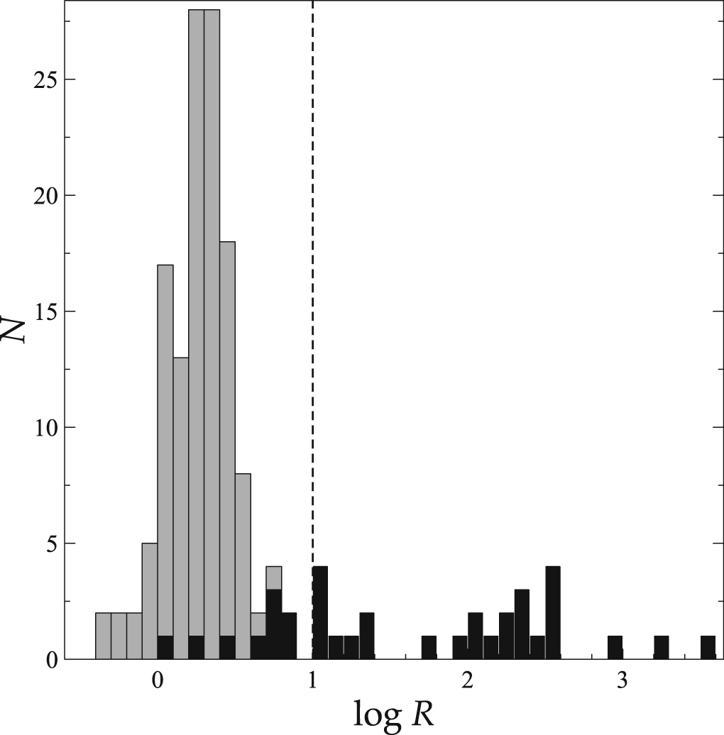
Standard image High-resolution imageIn summary, the GNIRS-DQS sources constitute an optically selected, NIR flux-limited sample of quasars, spanning wide ranges in rest-frame UV spectral properties, including broad absorption line (BAL) and non-radio-quiet quasars20 (comprising ∼30%21 and ∼12% of the sample, respectively; Pâris et al. 2018). Figure 3 shows the radio-loudness distribution of the GNIRS-DQS sources. The GNIRS-DQS sample is broadly representative of the general quasar population of luminous, high-redshift quasars during the epoch of most intense quasar activity (e.g., Hewett et al. 1993; Hasinger et al. 2005; Richards et al. 2006).

Figure 3. Radio-loudness distribution of the GNIRS-DQS sources; the shaded (gray) columns represent upper limits on R for radio undetected sources based on the Pâris et al. (2018) catalog, and the dashed line at log R = 1 indicates the threshold for radio-quiet quasars. This distribution is generally similar to that of the SDSS quasar population (e.g., Richards et al. 2006).
Download figure:
Standard image High-resolution image3. Observations and Data Reduction
The observations were designed to yield data of roughly comparable quality, in terms of both S/N and spectral resolution, to the respective SDSS spectra at λobs ∼ 5000 Å. The GNIRS spectra were thus required to have a ratio of ∼40 between the mean flux density and the standard deviation of that flux density in a rest-frame wavelength interval spanning 100 Å around λrest = 5100 Å, and a spectral resolution of R ∼ 1100 across the entire GNIRS band. These requirements enable accurate measurements of redshift based on [O iii] line peaks, with the high S/N contributing to reducing the uncertainties below the spectral resolution limit, ∼300 km s−1 (Shen et al. 2016). As explained below in Section 4, we determine that, on average, our spectra produce uncertainties on the measured line peak of [O iii] λ5007 of order ∼50 km s−1, stemming from pixel-to-wavelength calibration and our fitting procedures.
All spectra were obtained in queue-observing mode with GNIRS configured to use the Short Blue camera (0 15 pixel−1), the 32 lines mm−1 grating in cross-dispersed mode, and the 045 wide slit. This configuration covers the observed-frame ∼0.8–2.5 μm band in each source, simultaneously, in six spectral orders with overlapping spectral coverage. Our observing strategy utilized an ABBA method of slit nodding to enable sky subtraction. Exposure times ranged from ∼10 to 40 minutes for each object, with an additional 15 minutes of overhead per source. Each observation included calibration exposures, and either one or two ABBA sequences depending on source brightness. We also observed a telluric standard star either immediately before or after the observation in a spectral range of B8 V to A4 V, with 8200 K ≲ Teff ≲ 13,000 K, and typically within ≈10°–15° from each quasar.
The observation log of the original 272 sources appears in Table 1. Column (1) is the SDSS designation of the quasar. Column (2) provides the most reliable reported redshift estimate from SDSS (Pâris et al. 2018, Table A1, column 9 "Z"). Columns (3), (4), and (5) list the respective J, H, and K magnitudes of each quasar from the Two Micron All Sky Survey (2MASS; Skrutskie et al. 2006). Columns (6) and (7) give the observation date and semester, respectively. Column (8) is the net science exposure time, Column (9) provides comments, if any, concerning the observation, Column (10) provides a flag for whether or not the quasar is a BAL quasar (as defined in Pâris et al. 2018), and Column (11) provides a flag for whether or not the quasar is considered non-radio-quiet (see footnote 20).
Table 1. Observation Log
| Quasar | zSDSSa | J | H | K | Obs. Date | Semester | Net Exp. | Comments | BAL | RL |
|---|---|---|---|---|---|---|---|---|---|---|
| (mag) | (mag) | (mag) | (s) | |||||||
| (1) | (2) | (3) | (4) | (5) | (6) | (7) | (8) | (9) | (10) | (11) |
| SDSS J000544.71−044915.2 | 2.322 | 16.94 | 16.09 | 16.66 | 2019 Oct 18 | 2019B | 1800 | 4 | ⋯ | ⋯ |
| SDSS J000730.94−095831.5 | 2.223 | 17.09 | 15.94 | 15.37 | 2019 Jan 6 | 2018B | 1800 | ⋯ | 1 | ⋯ |
| SDSS J001249.89+285552.6 | 3.236 | 16.51 | 15.71 | 15.49 | 2017 Sep 9 | 2017B | 1800 | ⋯ | 1 | ⋯ |
| SDSS J001355.10−012304.0 | 3.396 | 16.71 | 16.05 | 15.46 | 2019 Jan 5 | 2018B | 900 | ⋯ | 1 | ⋯ |
| ⋯ | ⋯ | ⋯ | ⋯ | 2019 Jan 7 | 2018B | 900 | ⋯ | ⋯ | ⋯ | |
| SDSS J001453.20+091217.6 | 2.338 | 16.65 | 15.92 | 15.14 | 2017 Sep 19 | 2017B | 2025 | 1 | ⋯ | ⋯ |
| SDSS J001813.30+361058.6 | 2.316 | 16.15 | 15.65 | 14.75 | 2017 Aug 31 | 2017B | 1800 | ⋯ | ⋯ | ⋯ |
| SDSS J001914.46+155555.9 | 2.271 | 16.72 | 15.81 | 15.14 | 2017 Sep 1 | 2017B | 1800 | ⋯ | ⋯ | ⋯ |
| SDSS J002634.46+274015.5 | 2.250 | 17.05 | 15.92 | 15.25 | 2018 Dec 20 | 2018B | 1800 | ⋯ | ⋯ | ⋯ |
| SDSS J003416.61+002241.1 | 1.632 | 16.48 | 15.86 | 15.68 | 2017 Sep 1 | 2017B | 1800 | ⋯ | ⋯ | ⋯ |
Notes. Objects followed by an empty row aside from observation date, semester, and net exposure are additional observations made for that same object. Comments: (1) At least one exposure was taken under subpar observing conditions. (2) All exposures were taken under subpar observing conditions. (3) Supplemental data used from other observations to aid in reduction as described in Section 4.5. (4) Observation failed to provide spectrum of the source due to bad weather, instrument artifacts, or other technical difficulties during the observation.
aValue based on best available measurement as stated by SDSS (Pâris et al. 2018, Table A1, column 9 "Z").Only a portion of this table is shown here to demonstrate its form and content. A machine-readable version of the full table is available.
Download table as: DataTypeset image
We classify an acceptable observing night for this survey based on our programs' approved observing conditions including no more than 50% cloud cover and 85% image quality,22 however some objects were observed under worse conditions, and are noted as such in Table 1 (which brings the total number of lines in that table to 284). Additionally, 12 sources were observed over two observing sessions. These additional observations are recorded separately and immediately follow the initial observation in Table 1. For these objects, all available observations were utilized in the reduction process.
Our data-processing procedure generally follows the XDGNIRS pipeline developed by the Gemini Observatory (Mason et al. 2015 23 : see also Shen et al. 2019a) with the Gemini package in PyRAF.24 Following standard image cleaning for artifacts and other observational anomalies, we pair-subtract the images to remove the bulk of the background noise by directly combining the sky-subtracted object exposures. Quartz lamps and IR lamps were used to create flat fields to correct pixel-by-pixel variation across the detector. The flat-fielded images were corrected for optical distortions. Several objects required replacement flat fields due to pixel shifting of dead pixels in the detector into the GNIRS spectra directly (marked accordingly with a corresponding comment in Table 1), which produced a notable increase in the uncertainty of spectroscopic measurements for these objects, particularly in the bluer bands. On average, the increased flux uncertainty from these spectra is on the order of ∼3%. At this stage, of the 272 sources observed, 47 observations did not yield a meaningful spectrum due to bad weather, instrument artifacts, or other technical difficulties (Note 4 in Column 9 of Table 1), leaving the final sample at 226 sources.
Wavelength calibration was performed using two argon lamp exposures in order to assign wavelength values to the observed pixels. The uncertainties associated with this wavelength calibration are not larger than 0.5 Å rms, corresponding to ≲10 km s−1 at ∼15000 Å.
Spectra of the telluric standards were processed in a similar fashion, followed by a careful removal of the stars' intrinsic hydrogen absorption lines. This process was performed by fitting Lorentzian profiles to the hydrogen absorption lines, and interpolating across these features to connect the continuum on each side of the line. Following the line cancellation, the quasar spectra were divided by the corrected stellar spectra. The corrected spectra were multiplied by an artificial blackbody curve with a temperature corresponding to the telluric standard star, which yielded a cleaned, observed-frame quasar spectrum. Each quasar spectrum was flux calibrated by comparing local flux densities to the J, H, and K 2MASS magnitudes from Table 1 and using the magnitude-to-flux conversion factors from Table A.2 of Bessell et al. (1998). For the final spectra, we masked any noise present from cosmic rays, regions of high levels of atmospheric absorption, and band gap interference.
We chose this method as opposed to flux calibrating via the telluric standards to avoid any differences in atmospheric conditions between observations of the object and the telluric standard. This preference was also motivated by our use of a relatively narrow slit in order to prioritize spectral resolution at the cost of potentially larger slit losses in the observations. Although the 2MASS and Gemini observations are separated by several years in the quasars' rest frames, the cross-calibrations are subject to minimal uncertainties since ∼88% of our sources are luminous radio-quiet quasars at high redshift. Such sources typically show UV–optical flux variations on the order of ≲10% over such timescales (e.g., Vanden Berk et al. 2004; Kaspi et al. 2007; MacLeod et al. 2012). In fact, the effects stemming from the differences in airmass between the quasars and their respective telluric standard stars, as well as the slit losses, are typically larger than the expected intrinsic quasar variability.
In order to further test the reliability of our flux calibration, we compared the flux densities in overlapping continuum regions, λobs ∼ 8000–10000 Å, between our GNIRS spectra and those of the respective SDSS spectra; this test was feasible for ∼90% of our sources that have both high-quality GNIRS and SDSS spectral data where we can obtain meaningful comparisons that avoid reductions in quality that can occur in this region for both surveys. We found that the flux densities in the SDSS spectra are, on average, smaller than the GNIRS flux densities by ∼40% (μ = −0.155), with a 1σ scatter of ∼60% (σ = 0.2013) (see Figure 4, where μ and σ are the logarithms of the mean and standard deviation, respectively). Therefore, the flux densities when directly comparing both spectral sets are consistent at the 1σ level, despite the presence of this systematic offset. This systematic offset should be taken into account when comparing fluxes between SDSS and GNIRS spectra, however, it does not affect the emission-line measurements presented in this survey. This scatter may include discrepancies such as those due to intrinsic quasar variability, fiber light loss in SDSS spectra, and differences in airmass between quasars and their respective standard star observations. Examples of prominent emission lines in final, flux-calibrated spectra appear in Figure 5.

Figure 4. Flux-density ratio distribution between SDSS and GNIRS spectra from the overlapping continuum regions (λobs ∼ 8000–10000 Å) with a lognormal distribution fit. The log of the mean ratio (μ) and its standard deviation (σ) indicate that the flux densities of the GNIRS spectra are consistent at the 1σ level with those from their respective SDSS spectra.
Download figure:
Standard image High-resolution image
Figure 5. SDSS and GNIRS spectra and their best-fit models for three representative quasars in our sample (fitting of the SDSS spectra is deferred to a future publication). From left to right, panels show the corresponding SDSS spectra, followed by the GNIRS Mg ii, Hβ, and Hα spectral regions, respectively. In the three rightmost panels, the spectrum is presented by a thin solid line, and best-fit models for the localized linear continua, Gaussian profiles, and iron emission blends are marked by dashed lines. Summed best-fit model spectra are overplotted with thick solid lines. Details of the spectral fitting procedure are given in Section 4. All of the GNIRS spectra and their best-fit models are available electronically at http://physics.uwyo.edu/agn/GNIRS-DQS/spectra.html. We note that J083745.74+052109.4 is flagged as a BAL quasar (see Table 1 in Pâris et al. 2017), and will be discussed in a future publication.
Download figure:
Standard image High-resolution image4. Spectral Fitting
The final GNIRS quasar spectra were fit by using multiple localized linear continua, explained in Section 4.1, constrained by no less than six narrow (∼200 Å wide, rest-frame) line-free regions, and performing Gaussian fits to the emission lines. The Fe ii and Fe iii emission complexes were modeled via empirical templates from Boroson & Green (1992) and Vestergaard & Wilkes (2001) for the rest-frame optical and UV bands, respectively. These templates were scaled and broadened by convolving a Gaussian with an FWHM value that was free to vary between 1300 and 10,000 km s−1. Given that the Fe ii, Fe iii, and Hβ lines likely originate from different physical regions (e.g., Barth et al. 2013), we kept the FWHM of the iron templates as a free parameter. The FWHM values selected to broaden each template were determined using a least-squares analysis on each fitted region.
For the [O iii] lines, the widths of each line were restricted to be identical to each other, and their flux ratios were kept constant at I5007/I4959 = 3 (e.g., Storey & Zeippen 2000, and references therein); additionally, the rest-frame wavelength difference between the λ5007 and λ4959 lines was kept constant, which proved adequate for the fits of each object.
We fit two Gaussians to each broad emission-line profile to accommodate possible asymmetry present in the profile due to, e.g., absorption, or outflows. We note that the two Gaussians fit per broad emission line is adopted for fitting purposes only, and they do not represent physically distinct regions. Fitting the line profiles with more complex models was not warranted given the quality of our GNIRS spectra. The constraints on the Gaussian profiles for each emission line were that the peak wavelengths can differ from their known rest-frame values by up to ±1500 km s−1, on initial assessment (see, e.g., Richards et al. 2011, Figure 5) with a max flux value ranging from zero to a value calculated to be twice the maximum value of the emission line. Visual inspection yielded some exceptions beyond an offset of ±1500 km s−1, whereupon manual fitting was performed to compensate for the larger velocity offset.
4.1. Continuum Fitting
By using localized linear continuum fitting, we were able to achieve more accurate measurements by avoiding uncertainties stemming from a single power-law fit. There has been debate about an accurate model for quasar continua: a single power law, a broken power law (e.g., Vanden Berk et al. 2001), or whether the power-law description is appropriate at all in the rest-frame optical band; for example, in highly reddened quasar spectra a single power-law fitting will likely fail (see, e.g., Shen et al. 2019b). Alternatively, quasar continua may be better described by accretion disk modeling (e.g., Mejía-Restrepo et al. 2016). This survey was primarily concerned with measuring emission-line properties as opposed to continua, and, through using a variety of fitting methods including our own investigations into the efficacy of power-law and broken power-law fits, we conclude that localized linear continua give, at worst, the same level of uncertainty as power-law fitting, and, at best, avoid large uncertainties inherent in modeling blended continuum features. Therefore, measurements of all the emission lines implemented localized linear continua where the windows for fitting were determined by the availability of the nearest continuum band segments as defined in Vanden Berk et al. (2001).
4.2. Mg ii
The Mg ii doublet is detected in the bluer regions of our spectra, where the S/N is lower by roughly an order of magnitude than in the redder regions where the Hβ line is detected. Since our survey was designed such that the S/N near the Hβ region would be roughly comparable to the S/N across the respective SDSS spectrum of each source (see Section 2), the S/N around the Mg ii region in our GNIRS spectra is roughly an order of magnitude lower than the corresponding values in the SDSS spectra. As a result, we were only able to obtain reliable Mg ii and Fe ii+Fe iii fits for ∼31% of our sources (and we do not present measurements for Fe ii+Fe iii due to their considerable uncertainties). In this work, we only present Mg ii line measurements based on the GNIRS spectra of our sources; in a future publication, we will complement these data with Mg ii line measurements based on the sample's SDSS spectra (for ∼87% of our sample at z ≲ 2.4). On average, the uncertainties on the measured Mg ii properties are roughly an order of magnitude larger than those of Hβ. During the fitting process, we made a preliminary evaluation of the noise around the Hβ and Mg ii lines. If the noise around Mg ii was within a defined threshold (S/N ∼ 10) when compared to that of the Hβ region (S/N ∼ 40, see Section 3), the Mg ii line was fit automatically. Otherwise, each spectrum was visually inspected to determine if it was possible to perform reliable measurements of the Mg ii line. Due to the lower S/N in this region, the Fe ii+Fe iii complex was fit with narrow (∼20 Å) continuum bands and often required further interactive adjustments in order to avoid noise spikes to ensure accurate fitting to the Mg ii feature.
4.3. Hβ
The Hβ region, for most of our objects, provided reliable measurements given the survey was designed with this region in mind. However, in ≲2% of our objects, the Hβ emission line was adjacent to the edge of the observing band, resulting in larger uncertainties when fitting the Fe ii emission complex. This misalignment of Hβ stems from selecting our sample using UV-based redshifts, based primarily on the peak wavelength of the C iv emission line, which suffer from systematic biases due to outflows that can be as large as ≈5000 km s−1 (Dix et al. 2020; B. M. Matthews et al. 2021, in preparation). This misalignment also results in reduced coverage of the Fe ii blends for these objects. Despite this complication, we were able to adequately fit two Gaussians to each of the Hβ emission lines.
By design, our survey targeted highly luminous quasars, biased toward having higher L/LEdd values (see Figure 1 in Netzer 2003), which typically also tend to have relatively strong Fe ii emission. As a result, we relied on the broad iron bumps on either side of the Hβ line, rest frame ∼4450–4750 and 5100–5400 Å (Vanden Berk et al. 2001), as our primary region for fitting the Fe ii complex. While reasonable in most cases, these fits are likely affected by He ii λ4686 emission-line contamination, however the He ii emission line is unresolvable in this sample due to uncertainties from a variety of factors (see Section 4.5). On average, the corresponding Fe ii EW values in those sources is ∼20 Å. Additionally, ∼5% of our objects differed from the well-known trends of "Eigenvector 1" (Boroson & Green 1992), having a blend of strong [O iii] and Fe ii emission, resulting in their spectra exhibiting "shelves" on the red side of the Hβ profile. These features required a more careful fitting, and we did not see any evidence of [O iii] outflows directly contributing to this emission complex. An example of a shelf-like fit is presented in Figure 6.

Figure 6. GNIRS spectrum of the Hβ region of SDSS J001355.10-012304.0, zsys = 3.380. The "shelf" structure redward of the Hβ line appears to be a result of strong Fe ii and mild [O iii] emission. This differs from typical "Eigenvector 1" trends in Boroson & Green (1992), where sources with strong Fe ii blends tend to have weak [O iii] lines. Line styles are as in Figure 5. These shelves may be a signature of binary quasar candidates (see, e.g., Eracleous & Halpern 1994).
Download figure:
Standard image High-resolution imageFigure 7 shows the distribution of [O iii] EWs in the GNIRS-DQS sample. As explained in Section 4.6, for those objects that do not have detectable [O iii] emission, we must use the Mg ii line to determine systemic redshifts (zsys); for those objects that lack both [O iii] and Mg ii, we must utilize the Hβ line for that purpose, which is present in every GNIRS-DQS spectrum.

Figure 7. [O iii] rest-frame EW distribution of the GNIRS-DQS sources (gray) overplotted with rest-frame [O iii] EWs from Shen et al. (2011) (red outline; scaled down by a factor of 100). For ∼19% of the GNIRS-DQS sources that lack detectable [O iii] emission we are able to place strong upper limits on their EW values (black). When compared to [O iii] measurements of low-redshift, low-luminosity sources from Shen et al. (2011), the [O iii] emission tends to become weaker as luminosity increases, consistent with the trends observed in previous studies of high-redshift quasars (e.g., Netzer et al. 2004; Shen 2016).
Download figure:
Standard image High-resolution image
4.4. Hα
Being the most prominent feature in all the spectra of our sources at z < 2.5 (constituting ∼87% of the sample), Hα yielded the smallest uncertainties on all the emission-line parameters. We do not detect significant narrow [N ii] emission lines flanking the Hα line in any of our sources, which is expected given our selection of highly luminous quasars (e.g., Wills & Browne 1986; Shen et al. 2011).
4.5. Uncertainties in Spectral Measurements
The uncertainties inherent in the GNIRS spectra are contributed by a variety of factors. These include (but are not limited to) subpar observing conditions, the use of replacement flat fields in several of the spectra (see Section 3), and differences in airmass and/or atmospheric conditions between the standard star and the respective quasar observations. Moreover, modeling the telluric standard star continuum with a blackbody function fails to account for potential NIR excess emission from a circumstellar disk around the star. These factors lead to uncertainties on the flux density and shapes of the emission-line profiles, including the locations of their peaks. The uncertainties on these parameters are in the range ≈4%–7%, ≈3%–6%, ≈2%–5%, and ≈2%–4%, for each emission line, respectively. On average, these uncertainties result in general measurement errors across all parameters for an emission-line profile of up to ∼7%.
Emission-line fitting first relied on shifting the spectrum to the rest frame using the best available SDSS redshift. However, due to inaccuracies with the SDSS redshift, the emission lines in the GNIRS spectra often did not line up with the known rest-frame values. This offset led to uncertainties during fitting, and was ultimately mitigated by introducing a redshift iteration process. Emission-lines were fit for three different regimes separately, the Mg ii, Hβ, and Hα regions, based off of the SDSS redshift. A systemic redshift, zsys, was then determined by the best fit of the most reliable emission line for measuring redshift, as discussed in Section 4.6 below, and the spectrum was shifted according to this value. This process was repeated until the difference in consecutive redshifts was less than  for each region. Additionally, this redshift iteration allows more accurate measurements on zsys, the flux density at rest-frame 5100 Å (Fλ,5100), and more accurate fitting of the broadened iron templates.
After identifying the most accurate redshift, final fits are performed on emission-line features. Using preliminary Gaussian and localized linear continuum fits, residuals are generated, which yield upper and lower values for uncertainties present across the fitting region. With these residual bounds, Gaussian noise is introduced, and a series of 50 fits is performed in order to generate upper and lower bound estimates on the final Gaussian fits. To quantify the error on best-fit parameters, each iterated fit value is stored, which is used to generate a distribution of principle measurements. These distributions are then fit using a Gaussian function in order to determine the final errors at a 1σ confidence level. The iron templates of the Hβ and Mg ii regions also experience iterations of FWHM for the line profile, which allows for accurate Fe ii and Fe iii broadening error estimates. These various fitting iterations allow conservative error estimates on basic emission-line parameters, i.e., FWHM, EW, and line peaks. Finally, the best-fit spectral model for each source was verified by visual inspection.
4.6. The Catalog
Table 2 describes the format of the data presented in the catalog. The catalog contains basic emission-line properties, particularly FWHM and rest-frame EW, of the Mg ii, Hβ, [O iii], and Hα emission lines. The catalog also provides observed-frame wavelengths of emission-line peaks, as well as the asymmetry and kurtosis of each emission line, which were obtained from the Gaussian fits. A host of additional parameters are given, including the FWHM of the kernel Gaussian used for broadening the Fe ii blends around the Hβ region and the EW of these blends in the 4434–4684 Å region (following Boroson & Green 1992), as well as the flux density and monochromatic luminosity (λLλ) at 5100 Å. The catalog also provides zsys values measured from observed-frame wavelengths of emission-line peaks. For determining zsys, we adopt the observed-frame wavelength of the peak of one of three emission lines with the highest degree of accuracy which is present in the GNIRS spectrum, where it is known that these three emission lines have uncertainties of ≃50 km s−1, ≃200 km s−1, and ≃400 km s−1 for [O iii], Mg ii, and Hβ, respectively (Shen et al. 2016).
In cases where the prominent emission lines (i.e., Mg ii, Hβ, [O iii], and Hα) have no significant detections, upper limits are placed on their EWs by assuming FWHM values for each line using the median value in the sample distributions, and taking the weakest feature detectable in the GNIRS spectra for each line. Additionally, we placed upper limits on the EW of the optical Fe II blends in cases where excess noise surrounding the Hβ + [O iii] region would not enable us to fit the Fe ii blends reliably; we found that a value of 2 Å for this parameter provides a conservative upper limit in all such cases.
Table 2. Column Headings for Spectral Measurements
| Column | Name | Units | Description |
|---|---|---|---|
| 1 | OBJ | ⋯ | SDSS object designation |
| 2 | ZSYS | ⋯ | Systemic redshifts |
| 3 | LC_MG II | Å | Observed-frame wavelength of the emission-line peak of Mg ii based on peak fit value |
| 4 | LC_MG II_UPP | Å | Upper uncertainty for the line peak of Mg ii |
| 5 | LC_MG II_LOW | Å | Lower uncertainty for the line peak of Mg ii |
| 6 | FWHM_MG II | km s−1 | FWHM of Mg ii |
| 7 | FWHM_MG II_UPP | km s−1 | Upper uncertainty of FWHM of Mg ii |
| 8 | FWHM_MG II_LOW | km s−1 | Lower uncertainty of FWHM of Mg ii |
| 9 | EW_MG II | Å | Rest-frame EW of Mg ii |
| 10 | EW_MG II_UPP | Å | Upper uncertainty of EW of Mg ii |
| 11 | EW_MG II_LOW | Å | Lower uncertainty of EW of Mg ii |
| 12 | AS_MG II | ⋯ | Asymmetry of the double Gaussian fit profile of Mg ii |
| 13 | KURT_MG II | ⋯ | Kurtosis of the double Gaussian fit profile of Mg ii |
| 14 | LC_HB | Å | Observed-frame wavelength of the emission-line peak of Hβ based on peak fit value |
| 15 | LC_HB_UPP | Å | Upper uncertainty for the line peak of Hβ |
| 16 | LC_HB_LOW | Å | Lower uncertainty for the line peak of Hβ |
| 17 | FWHM_HB | km s−1 | FWHM of Hβ |
| 18 | FWHM_HB_UPP | km s−1 | Upper uncertainty of FWHM of Hβ |
| 19 | FWHM_HB_LOW | km s−1 | Lower uncertainty of FWHM of Hβ |
| 20 | EW_HB | Å | Rest-frame EW of Hβ |
| 21 | EW_HB_UPP | Å | Upper uncertainty of EW of Hβ |
| 22 | EW_HB_LOW | Å | Lower uncertainty of EW of Hβ |
| 23 | AS_HB | ⋯ | Asymmetry of the double Gaussian fit profile of Hβ |
| 24 | KURT_HB | ⋯ | Kurtosis of the double Gaussian fit profile of Hβ |
| 25 | LC_O III | Å | Observed-frame wavelength of the emission-line peak of [O iii] λ5007 based on peak fit value |
| 26 | LC_O III_UPP | Å | Upper uncertainty for the line peak of [O iii] λ5007 |
| 27 | LC_O III_LOW | Å | Lower uncertainty for the line peak of [O iii] λ5007 |
| 28 | FWHM_O III | km s−1 | FWHM of [O iii] λ5007 |
| 29 | FWHM_O III_UPP | km s−1 | Upper uncertainty of FWHM of [O iii] λ5007 |
| 30 | FWHM_O III_LOW | km s−1 | Lower uncertainty of FWHM of [O iii] λ5007 |
| 31 | EW_O III | Å | Rest-frame EW of [O iii] λ5007 |
| 32 | EW_O III_UPP | Å | Upper uncertainty of EW of [O iii] λ5007 |
| 33 | EW_O III_LOW | Å | Lower uncertainty of EW of [O iii] λ5007 |
| 34 | AS_O III | ⋯ | Asymmetry of the double Gaussian fit profile of [O iii] λ5007 |
| 35 | KURT_O III | ⋯ | Kurtosis of the double Gaussian fit profile of [O iii] λ5007 |
| 36 | LC_HA | Å | Observed-frame wavelength of the emission-line peak of Hα based on peak fit value |
| 37 | LC_HA_UPP | Å | Upper uncertainty for the line peak of Hα |
| 38 | LC_HA_LOW | Å | Lower uncertainty for the line peak of Hα |
| 39 | FWHM_HA | km s−1 | FWHM of Hα |
| 40 | FWHM_HA_UPP | km s−1 | Upper uncertainty of FWHM of Hα |
| 41 | FWHM_HA_LOW | km s−1 | Lower uncertainty of FWHM of Hα |
| 42 | EW_HA | Å | Rest-frame EW of Hα |
| 43 | EW_HA_UPP | Å | Upper uncertainty of EW of Hα |
| 44 | EW_HA_LOW | Å | Lower uncertainty of EW of Hα |
| 45 | AS_HA | ⋯ | Asymmetry of the double Gaussian fit profile of Hα |
| 46 | KURT_HA | ⋯ | Kurtosis of the double Gaussian fit profile of Hα |
| 47 | FWHM_FE II | km s−1 | FWHM of the kernel Gaussian used to broaden the Fe ii template |
| 48 | EW_FE IIa | Å | Rest-frame EW of Fe ii in the optical as defined by Boroson & Green (1992) |
| 49 | LOGFλ5100 | erg s−1 cm−2 Å−1 | Flux density at rest-frame 5100 Å |
| 50 | LOGL5100 | erg s−1 | Monochromatic luminosity at rest-frame 5100 Å |
Note. Data formatting used for the catalog. Asymmetry is defined here as the skewness of the Gaussian fits, i.e., a measure of the asymmetry of the distribution about its mean,  , where μ is the mean of x, σ is the standard deviation of x, and E(t) is the expectation value. Kurtosis is the quantification of the "tails" of the Gaussian fits defined as
  , where symbols are the same as for asymmetry.
Only a portion of this table is shown here to demonstrate its form and content. A machine-readable version of the full table is available.
Download table as: DataTypeset image
Finally, additional, and typically weaker, emission-line measurements follow the formatting presented in Table 3, and are reported in the supplemental features catalog for 106 sources from our sample where such features could be measured reliably. These emission lines were fit on a case-by-case basis after visually inspecting each GNIRS spectrum (and no upper limits are assigned in cases of nondetections). Where applicable, we performed fits on the following emission lines with two Gaussians per line, following the same methodology used for primary emission-line measurements: Hδ λ4101, Hγ λ4340, and [Ne iii] λ3871. The [O ii] λ3727 doublet was fit in the same manner.
Table 3. Column Headings for Supplemental Emission-line Measurements
| Column | Name | Units | Description |
|---|---|---|---|
| 1 | OBJ | ⋯ | SDSS object designation |
| 2 | LC_HD | Å | Observed-frame wavelength of the emission-line peak of Hδ based on peak fit value |
| 3 | LC_HD_UPP | Å | Upper uncertainty for the line peak of Hδ |
| 4 | LC_HD_LOW | Å | Lower uncertainty for the line peak of Hδ |
| 5 | FWHM_HD | km s−1 | FWHM of Hδ |
| 6 | FWHM_HD_UPP | km s−1 | Upper uncertainty of FWHM of Hδ |
| 7 | FWHM_HD_LOW | km s−1 | Lower uncertainty of FWHM of Hδ |
| 8 | EW_HD | Å | Rest-frame EW of Hδ |
| 9 | EW_HD_UPP | Å | Upper uncertainty of EW of Hδ |
| 10 | EW_HD_LOW | Å | Lower uncertainty of EW of Hδ |
| 11 | AS_HD | ⋯ | Asymmetry of the double Gaussian fit profile of Hδ |
| 12 | KURT_HD | ⋯ | Kurtosis of the double Gaussian fit profile of Hδ |
| 13 | LC_HG | Å | Observed-frame wavelength of the emission-line peak of Hγ based on peak fit value |
| 14 | LC_HG_UPP | Å | Upper uncertainty for the line peak of Hγ |
| 15 | LC_HG_LOW | Å | Lower uncertainty for the line peak of Hγ |
| 16 | FWHM_HG | km s−1 | FWHM of Hγ |
| 17 | FWHM_HG_UPP | km s−1 | Upper uncertainty of FWHM of Hγ |
| 18 | FWHM_HG_LOW | km s−1 | Lower uncertainty of FWHM of Hγ |
| 19 | EW_HG | Å | Rest-frame EW of Hγ |
| 20 | EW_HG_UPP | Å | Upper uncertainty of EW of Hγ |
| 21 | EW_HG_LOW | Å | Lower uncertainty of EW of Hγ |
| 22 | AS_HG | ⋯ | Asymmetry of the double Gaussian fit profile of Hγ |
| 23 | KURT_HG | ⋯ | Kurtosis of the double Gaussian fit profile of Hγ |
| 24 | LC_O IIa | Å | Observed-frame wavelength of the emission-line peak of [O ii] based on peak fit value |
| 25 | LC_O II_UPP | Å | Upper uncertainty for the line peak of [O ii] |
| 26 | LC_O II_LOW | Å | Lower uncertainty for the line peak of [O ii] |
| 27 | FWHM_O II | km s−1 | FWHM of [O ii] |
| 28 | FWHM_O II_UPP | km s−1 | Upper uncertainty of FWHM of [O ii] |
| 29 | FWHM_O II_LOW | km s−1 | Lower uncertainty of FWHM of [O ii] |
| 30 | EW_O II | Å | Rest-frame EW of [O ii] |
| 31 | EW_O II_UPP | Å | Upper uncertainty of EW of [O ii] |
| 32 | EW_O II_LOW | Å | Lower uncertainty of EW of [O ii] |
| 33 | AS_O II | ⋯ | Asymmetry of the double Gaussian fit profile of [O ii] |
| 34 | KURT_O II | ⋯ | Kurtosis of the double Gaussian fit profile of [O ii] |
| 35 | LC_NE IIIb | Å | Observed-frame wavelength of the emission-line peak of [Ne iii] based on peak fit value |
| 36 | LC_NE III_UPP | Å | Upper uncertainty for the line peak of [Ne iii] |
| 37 | LC_NE III_LOW | Å | Lower uncertainty for the line peak of [Ne iii] |
| 38 | FWHM_NE III | km s−1 | FWHM of [Ne iii] |
| 39 | FWHM_NE III_UPP | km s−1 | Upper uncertainty of FWHM of [Ne iii] |
| 40 | FWHM_NE III_LOW | km s−1 | Lower uncertainty of FWHM of [Ne iii] |
| 41 | EW_NE III | Å | Rest-frame EW of [Ne iii] |
| 42 | EW_NE III_UPP | Å | Upper uncertainty of EW of [Ne iii] |
| 43 | EW_NE III_LOW | Å | Lower uncertainty of EW of [Ne iii] |
| 44 | AS_NE III | ⋯ | Asymmetry of the double Gaussian fit profile of [Ne iii] |
| 45 | KURT_NE III | ⋯ | Kurtosis of the double Gaussian fit profile of [Ne iii] |
Notes. Data formatting used for the supplemental measurements in the supplemental features catalog.
a[O ii] λ3727. b[Ne iii] λ3870.Only a portion of this table is shown here to demonstrate its form and content. A machine-readable version of the full table is available.
Download table as: DataTypeset image
5. Summary
We present a catalog of spectroscopic properties obtained from NIR observations of a uniform, flux-limited sample of 226 SDSS quasars at 1.5 ≲ z ≲ 3.5, which is the largest uniform inventory for such sources to date. The catalog includes basic spectral properties of Mg ii, Hβ, [O iii], Fe ii, and Hα emission lines, as well as Hδ, Hγ, [O ii], and [Ne iii] emission lines for a subset of the sample. A spectral resolution of R ∼ 1100 was achieved for this data set, which is roughly comparable to the value of the corresponding SDSS spectra. These measurements provide a database to comprehensively analyze and investigate rest-frame UV–optical spectral properties for high-redshift, high-luminosity quasars in a manner consistent with studies of low-redshift quasars.
In particular, the catalog will enable future work on robust calibrations of UV-based proxies to systemic redshifts and black hole masses in distant quasars. Such prescriptions are becoming increasingly more important as millions of quasar optical spectra will be obtained in the near future by, e.g., the Dark Energy Spectroscopic Instrument (DESI; Levi et al. 2013; DESI Collaboration et al. 2016) and the 4 m Multi-Object Spectroscopic Telescope (de Jong et al. 2012), where reliable estimates of zsys and MBH will be crucial to extract the science value from these surveys. In forthcoming papers we will present, among other facets, redshift calibrations via indicative emission lines such as [O iii] (B. M. Matthews et al. 2021, in preparation), SMBH estimates using the Hβ and Mg ii profiles measured in this survey (C. Dix et al. 2021, in preparation), and correlations among UV–optical emission lines (e.g., Boroson & Green 1992; Wills et al. 1999; Shen & Liu 2012).
In the future, we should continue to push the redshift barrier for the Hβ and [O iii] emission lines, as current investigations have been confined to z ≲ 3.5, in order to gain an increased understanding of the coevolution of SMBHs and their host galaxies, along with more reliable redshifts. However, at redshifts higher than z ∼ 3.5, these observations cannot be obtained via ground-based telescopes. Future studies in this respect could include a two-pronged approach using small calibration surveys. The first survey, for example, can use higher resolution instruments such as Gemini's Spectrograph and Camera for Observations of Rapid Phenomena in the Infrared and Optical (SCORPIO; Robberto et al. 2018) which will better measure weak emission-line profiles and obtain more accurate measurements of the prominent emission lines. This information will reinforce the measurements of this survey and allow for more confident applications to much higher redshifts, even beyond z > 6. The second survey would be a select sample of a few dozen highly luminous z > 3.5 objects using space-based observations from the James Webb Space Telescope (Gardner et al. 2006) for optimal spectral quality, with the possibility for a contemporaneous SCORPIO survey to obtain measurements of lines such as C iv from the ground.
This work is supported by National Science Foundation grants AST-1815281 (B.M.M., O.S., C.D.), AST-1815645 (M.S.B., A.D.M.), AST-1516784 (W.N.B.), and AST-1715579 (Y.S.). A.D.M. was also supported, in part, by the Director, Office of Science, Office of High Energy Physics of the U.S. Department of Energy under Award No. DE-SC0019022. Y.S. acknowledges support from an Alfred P. Sloan Research Fellowship. We thank an anonymous referee for thoughtful and valuable comments that helped improve this manuscript. This research has made use of the NASA/IPAC Extragalactic Database (NED), which is operated by the Jet Propulsion Laboratory, California Institute of Technology, under contract with the National Aeronautics and Space Administration. We thank Jin Wu and the Gemini Observatory staff for helpful discussions, and providing assistance with data reduction for this project. This work was enabled by observations made from the Gemini North telescope, located within the Maunakea Science Reserve and adjacent to the summit of Maunakea. We are grateful for the privilege of observing the universe from a place that is unique in both its astronomical quality and its cultural significance.
Footnotes
- 19
- 20
We consider radio-quiet quasars to have R < 10, where R is the radio loudness, defined as R = fν(5 GHz)/fν (4400 Å), where fν(5 GHz) and fν(4400 Å) are the flux densities at rest-frame frequencies of 5 GHz and 4400 Å, respectively (Kellermann et al. 1989). Non-radio-quiet quasars include radio-intermediate (10 < R < 100) and radio-loud (R > 100) sources, respectively.
- 21
- 22
- 23
- 24