Effects of Multiconstituent Tides on a Subterranean Estuary With Fixed-Head Inland Boundary

Highlights

Salinity distributions fluctuated intensively as the inland aquifer extent decreased.

Aquifer of a shorter inland aquifer extent smoothed out fewer tidal constituents.

Inland aquifer extent regulated the tidal effects on salinity distributions.

Introduction

Ocean tides are identified as an important driving force that controls the hydrodynamic and biogeochemical processes in coastal aquifers (Werner et al., 2013; Robinson et al., 2018). In subterranean estuaries (i.e., mixing zones between terrestrially derived fresh groundwater and recirculating seawater in coastal aquifers), tides significantly affect submarine groundwater discharge (SGD) and salinity distributions (Werner et al., 2013; Robinson et al., 2018). Tidal forcing, in combination with the density contrast between terrestrial fresh groundwater and nearshore seawater, can lead to the formation of two saltwater recirculation zones in unconfined aquifers: a lower saltwater wedge (SW) and an upper saline plume (USP) (Boufadel, 2000; Robinson et al., 2006).

While tidal effects on SGD and salinity distributions in subterranean estuaries have been studied extensively, previous studies predominately considered single-frequency (monochromatic) tides (Robinson et al., 2007b; Kuan et al., 2019; Shen et al., 2019; Yu et al., 2019a), bichromatic spring-neap tides (Robinson et al., 2007a; Abarca et al., 2013; Heiss and Michael, 2014; Buquet et al., 2016), or fitted tidal variations with several primary constituents (Levanon et al., 2016; Geng and Boufadel, 2017; Levanon et al., 2017; Yu et al., 2019b). Coastal aquifer systems are commonly subjected to oceanic tidal fluctuations, which likely contain tens of constituents with different fluctuation frequencies and amplitudes (Pawlowicz et al., 2002). This would lead to complex and irregular SGD and salinity distributions.

Recently, Yu et al. (2019b) numerically examined the effect of multiconstituent tides on both SGD and salinity distributions in a subterranean estuary. They found that the response of water exchange (e.g., SGD) across the aquifer-sea interface to tides is almost instantaneous. As such, the present (at any given moment) water exchange is mainly influenced by the present (i.e., at the same time) tidal conditions. However, the response of salinity distributions to tides is delayed; thus, salinity distributions are dependent on the antecedent (previous) tidal conditions.

Yu et al. (2019b) found that coastal aquifers behave as a low-pass filter smoothing-out tidal signals, particularly high-frequency tidal constituents (e.g., semidiurnal and diurnal tidal signals). Furthermore, the combination of high-frequency tidal constituents generates new low-frequency signals when the tidal signals propagate in the aquifer, as determined by Li et al. (2000) using analytical solutions for groundwater tidal propagation. These generated low-frequency signals, combined with the primary tidal fluctuations created directly by the ocean tide, jointly affect the salinity distributions (e.g., SW and USP) in unconfined aquifers (Yu et al., 2019b). With the antecedent tidal conditions weighted in the form of convolution using the probability density function of the Gamma distribution, Yu et al. (2019b) demonstrated that the prolonged and cumulative effects of antecedent tidal conditions on the present salinity distributions in unconfined aquifers could be quantified.

Yu et al. (2019b) studied multiconstituent tides within a coastal unconfined aquifer with a fixed-flux inland boundary and inland extent of 150 m. Both fixed-flux (Michael et al., 2005; Robinson et al., 2007c; Kuan et al., 2012; Evans and Wilson, 2016) and fixed-head (Li et al., 1997; Ataie-Ashtiani et al., 1999; Heiss and Michael, 2014; Geng and Boufadel, 2015) inland boundaries have been widely adopted in previous studies of SGD and salinity distributions. The former assumes that freshwater discharge to the sea is constant, whereas the latter applies to topography-controlled aquifers (Werner and Simmons, 2009; Michael et al., 2013). In low-elevation coastal areas, the watertable is often shallow, leading to the overlying unsaturated zone being thin. Under this condition, the rainfall-induced infiltration would be inhibited, i.e., once the soil is saturated, surface water runoff would occur and the watertable tends to be fixed to the local surface elevation. This likely forms a fixed-head inland boundary (Michael et al., 2013; Sawyer et al., 2016). Michael et al. (2013) suggested that approximately 70% of the world’s coastlines are topography-controlled. Coastal aquifers with fixed-head landward boundaries are recognized to be more vulnerable to seawater intrusion, as salinity distributions are more responsive to changes to ocean boundary conditions (Werner and Simmons, 2009; Michael et al., 2013). Despite the commonality of fixed-head inland boundaries, the question remains open as to how they regulate the SGD and salinity distributions in subterranean estuaries subjected to multiconstituent tides.

In this study, we focused on the effects of multiconstituent tides on SGD and salinity distributions in unconfined aquifers with fixed-head inland boundaries at different landward positions, under the assumption that the yearly averaged inland freshwater input is the same in aquifers of alternative landward extent. The following key questions were explored based on numerical simulations: 1) How does a change in the inland aquifer extent affect the SGD and salinity distribution responses to multiconstituent tides? 2) How do multiconstituent tides affect inland freshwater input in inland fixed-head aquifers? 3) How does the inland aquifer extent influence the role of antecedent tidal conditions on salinity distributions?

Conceptual Model and Simulations

Similar to Yu et al. (2019b), a 2D cross-shore section of a coastal unconfined aquifer was considered in this study, as shown in Figure 1. Boundary DEF was set as the time-variant head boundary (aquifer-sea interface) affected by multiconstituent tides. To investigate the response of the aquifer to multiconstituent tides, we used six years (2011–2016) of real tide data measured from Brisbane Bar tidal station (website: http://data.qld.gov.au/dataset/brisbane-bar-tide-gauge-archived-interval-recordings). The measurement interval was 600 s. Four dominant tidal constituents were detected in this dataset based on spectral analysis: 1) principal lunar semidiurnal tidal constituent (M₂, T (tidal period) = 12.42 h, A (tidal amplitude) = 0.73 m); 2) principal solar semidiurnal tidal constituent (S₂, T = 12 h, A = 0.19 m); 3) lunisolar declinational diurnal tidal constituent (K₁, T = 23.93 h, A = 0.19 m); 4) larger lunar elliptic semidiurnal tidal constituent (N₂, T = 12.66 h, A = 0.15 m).

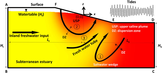
FIGURE 1. Conceptual diagram of a subterranean estuary of an unconfined aquifer. Flow processes considered in this article are as follows: 1) density-driven seawater circulation, 2) tide-induced seawater circulation, and 3) terrestrial groundwater discharge. The colors represent the salinity (yellow for freshwater and red for saltwater). Boundary ABCDEF represents the model domain. The x-z coordinate origin was set at the mean shoreline. L_I and L_S are the inland and seaward aquifer extents, respectively. H_I and H_S are the inland and seaward aquifer thicknesses, respectively. H_f is inland watertable elevation at the inland boundary.

Boundaries BC and CD were set to no-flow boundaries. Rainfall and evaporation were excluded and thus AF was also set as a no-flow boundary. Different from Yu et al. (2019b), the landward boundary AB was set to a fixed-head boundary. The fresh groundwater recharged from the inland boundary AB and discharged into the ocean through the aquifer-sea interface DEF. It is worth noting that to make the simulation results comparable, inland watertable elevations (H_f) were adjusted to get a similar yearly averaged freshwater input (around 2.1 m³/m/d). We focused on four cases with the fixed-head inland boundary located at different locations as follows:

Fixed-head and L_I = 50 m (L_I is the inland aquifer extent, which measures the horizotal distance from the inland boundary to the shoreline), with the seaward aquifer extent L_S = 50 m, the seaward aquifer thickness H_S = 27 m, and the inland aquifer thickness H_I = 33 m (note that the same L_S, H_S, and H_I were set in all the cases). H_f was fixed at 0.81 m.

Fixed-head and L_I = 100 m, H_f was fixed at 1.15 m.

Fixed-head and L_I = 150 m, H_f was fixed at 1.50 m.

Fixed-head and L_I = 200 m, H_f was fixed at 1.83 m.

In addition to these four cases with fixed-head inland boundaries, one case with fixed-flux inland boundary (L_I = 150 m, similar to that used in Yu et al. (2019b)) was also considered for comparing the behavior of aquifers with different inland boundaries. We tested the effect of inland aquifer extent (L_I) on salinity distributions in the aquifers with fixed-flux inland boundaries. The results showed that the inland aquifer extent did not remarkably affect the variation of the USP and SW in the aquifers. Therefore, only the results from one case with fixed-flux inland boundary (fixed-flux and L_I = 150 m) were included in this article. The aquifer properties were similar to those used in Yu et al. (2019b). That is, the model setup was based on a homogeneous sandy beach with hydraulic conductivity K_s = 10 m/d and porosity ϕ = 0.45. The beach slope was 0.1. The longitudinal and transverse dispersivities were set to 0.5 and 0.05 m, respectively (Hunt et al., 2011). The residual water saturation S_Wres was set to 0.1 and water retention parameters α and n were set to 14.5 m⁻¹ and 2.68 (typical values for sand (Carsel and Parrish, 1988)) for the van Genuchten (1980) equations.

The numerical simulations were conducted using SUTRA (Voss and Provost, 2010), which simulates variably saturated and density-dependent pore-water flow and associated solute transport. In the inland subdomain, a mesh with ∆x = 1.5 m and ∆z = 0.5 m was used, while in the intertidal and seabed subdomain, the mesh was refined (∆x ≈ 0.33 m and ∆z ≈ 0.1 m). For all the simulations, the model was initially run to the steady states (pressure and salinity unchanged) with a static sea level (0 m). The measured tidal conditions (2011–2016) were then introduced as the boundary conditions in the model with a time step of 300 s. Here, we focused on the analysis of the last two years (2015–2016). As suggested by Yu et al. (2019b) and will be discussed later, after 4 years (2011–2014), the behavior of the system was independent of the initial conditions subjected to the static sea level.

Results and Analysis

SGD and Salinity Distribution Fluctuations Induced by the Multiconstituent Tides

As mentioned earlier, for the five considered cases (four with fixed-head inland boundaries and one with fixed-flux inland boundary), the averaged inland freshwater input was similar. The two-year (2015–2016) averaged salinity distributions in the aquifers were similar for the five cases, e.g., the 50% isohaline of the seawater (17.5 ppt) largely overlapped (Figure 2). This suggests that the yearly averaged inland freshwater input rather than the inland aquifer extent significantly affected the salinity distributions at a long-time scale. For the four cases with fixed-head inland boundaries, the calculated yearly averaged amounts of salt stored in (per unit width) saltwater wedge (SM_SW) and upper saline plume (SM_USP) were also close to those for the case with fixed-flux inland boundary (8,425 and 872 kg/m, respectively) (Table 1). The averaged tide-induced (around 1.4 m³/m/d) and density-driven (around 1 m³/m/d) seawater circulation fluxes were also similar for all the cases (Table 1). Since the yearly averaged inland freshwater input was similar, the inland aquifer extent did not remarkably affect the averaged SGD and salinity distributions in the aquifers subjected to the multiconstituent tides.

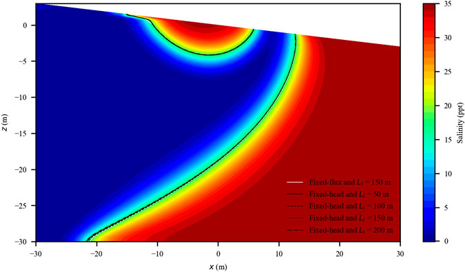
FIGURE 2. Two-year averaged salinity distribution in the aquifer (note that only the beach section is presented). The salinity is shown by different colors (the case of fixed-head (L_I = 50 m) was used). The different types of lines represent the 50% isohaline of the seawater for the different cases (largely overlapped). The salinity distributions are similar in the cases with fixed-flux (L_I = 150 m) and fixed-head (L_I = 50, 100, 150, and 200 m) inland boundaries.

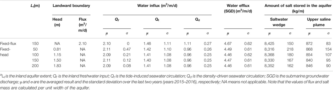
TABLE 1. Key results of the flux and salinity distributions affected by different inland boundaries^a.

We further investigated the variation of fluxes and salinity distributions (both water flux and amount of salt stored) in response to the multiconstituent tides by presenting the variation in the last two years (2015–2016). To quantify the fluctuations for the different cases, the averaged value (μ) and the standard deviation (σ) over each principal semidiurnal lunar tidal cycle (12.42 h) in these two years were calculated.

The calculated standard deviations for the tide-induced and density-driven influx were similar among the four cases with fixed-head inland boundaries and differed slightly from that for the case with fixed-flux inland boundary (Table 1). The SGD, as the total efflux across the aquifer-sea interface, varied intensively in response to the multiconstituent tides (Figure 3). The averaged values of the SGD over each principal semidiurnal lunar tidal cycle for the five cases largely overlapped. Consistently, the calculated standard deviations were quite similar and around 0.62 m³/m/d. This suggests that, for the simulated cases with similar averaged freshwater input, SGD was predominantly affected by the present tidal conditions. The response of SGD to the tidal fluctuations was mostly instantaneous; thus, the effect of the inland aquifer extent was not obvious.

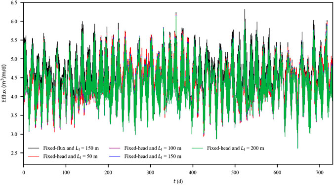
FIGURE 3. Averaged per unit width water efflux (i.e., submarine groundwater discharge) every 12.42 h for the cases with fixed-flux (L_I = 150 m) and fixed-head (L_I = 50, 100, 150, and 200 m) inland boundaries. Note that the lines are largely overlapped.

In contrast, the fluctuations of freshwater input differed case by case (Figure 4). As the inland aquifer extent decreased, the averaged values of the freshwater input over each principal semidiurnal lunar tidal cycle started to fluctuate around that for the case with fixed-flux inland boundary (2.1 m³/m/d). As L_I reduced from 200 to 150, 100, and 50 m, the standard deviation increased from 0.08 to 0.12, 0.21, and 0.47 m³/m/d, respectively. It is worth noting that the equal reduction in L_I led to unequal increase in the standard deviation of the freshwater input, leading to an accelerating trend. The inland freshwater input was controlled by the lateral hydraulic gradient. As setup in the simulations, a similar yearly averaged inland freshwater input was produced (Table 1). It is expected that the instantaneous hydraulic gradient was continuously modified by the inland watertable and seaward tidal level. The multiple tidal constituents propagated into the aquifer and thus affected the hydraulic gradient in a complex fashion. In particular, the low-frequency signals would propagate further inland and obviously affect the freshwater input (details in Analysis on Amplitude Spectrums).

FIGURE 4. Averaged inland freshwater input every 12.42 h for the cases with fixed-flux (L_I = 150 m) and fixed-head (L_I = 50, 100, 150, and 200 m) inland boundaries.

For both the cases with fixed-head and fixed-flux inland boundaries, SM_SW and SM_USP fluctuated remarkably (Figures 5, 6). Overall, the cases with fixed-head inland boundaries were related to intensive fluctuations in the averaged value over each principal semidiurnal lunar tidal cycle (Table 1). As L_I reduced from 200 to 150, 100, and 50 m, the standard deviation for SM_SW increased from 162 to 167, 180, and 218 kg/m, respectively, whereas the standard deviation for SM_USP increased from 90 to 95, 107, and 154 kg/m, respectively. Clearly, the fluctuation intensity for SM_SW was more obvious than that for SM_USP, suggesting that SM_SW tended to be more affected by the low-frequency tidal signals (details in Analysis on Amplitude Spectrums).

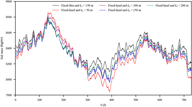
FIGURE 5. Averaged amount of salt stored in the saltwater wedge every 12.42 h for the cases with fixed-flux (L_I = 150 m) and fixed-head (L_I = 50, 100, 150, and 200 m) inland boundaries.

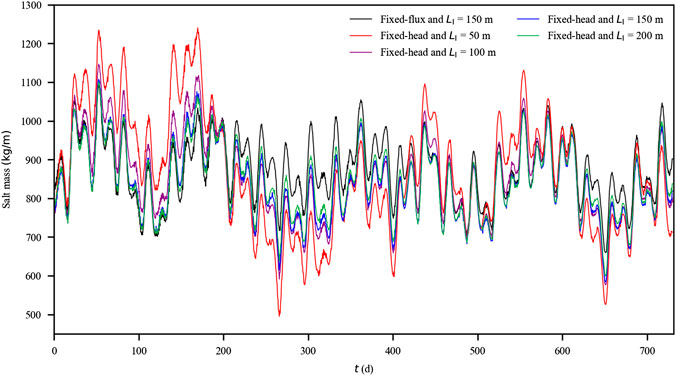
FIGURE 6. Averaged amount of salt stored in the upper saline plume every 12.42 h for the cases with fixed-flux (L_I = 150 m) and fixed-head (L_I = 50, 100, 150, and 200 m) inland boundaries.

Analysis of Amplitude Spectra

The variations of the SGD and salinity distributions could be reflected by amplitude spectra. Similar to Yu et al. (2019b), the instantaneous results were selected with a 2 h time interval (X). We also used the following standardized and nondimensional variables (X*).

As expected, four dominant frequencies (M₂, S₂, K₁, and N₂) appeared in the tidal series (Figure 7A) and also in the SGD variations (Figure 7B). As pointed out by Yu et al. (2019b), in the SGD, two new signals with frequencies of 7.83 × 10^–7 Hz (spring-neap tidal cycle, 14.8-day period) and 4.24 × 10^–7 Hz (27.3-day period) were generated by the combinations of M₂ and S₂ tidal constituents (f (S₂)−f (M₂)) and M₂ and N₂ tidal constituents (f (M₂)−f (N₂)), respectively. These two new signals also appeared in the freshwater input, SM_SW and SM_USP (Figures 7C–E).

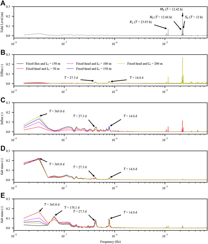
FIGURE 7. Amplitude spectra of (A) tidal level variation, (B) submarine groundwater discharge (SGD), (C) inland freshwater input, (D) amount of salt stored in the saltwater wedge (SM_SW), and (E) amount of salt stored in the upper saline plume (SM_USP). The results are standardized.

Different from the tidal and SGD series, the low-frequency signals started to play important roles in the freshwater input, SM_SW and SM_USP (Figures 7C–E). The contributions (defined as the ratio of a specific nondimensional amplitude to the sum of all the nondimensional amplitudes) of these signals changed in different ways as L_I reduced. For example, for the freshwater input, the contribution of the signal of the 365-day period decreased from 7.21% to 6.10%, 4.51%, and 1.83% as L_I reduced from 200 to 150, 100, and 50 m, respectively. The contribution of the signal of the 365-day period kept unchanged for SM_SW, whereas for SM_USP, it increased from 2.44% to 3.43%, 5.35%, and 9.33% as L_I reduced from 200 to 150, 100, and 50 m, respectively.

As mentioned earlier, the low-frequency signals likely propagated further landward and thus interacted more with the inland boundary. The boundary reflections would damp these signals. The extent of damping depended on the inland aquifer extent and the tidal frequencies. With respect to the variation of the freshwater input, the low-frequency signal of the 365-day period was not apparent with L_I = 50 m, where the high-frequency signals (M₂, S₂, K₁, and N₂) were relatively strong. Thus, the fluctuation intensity of the freshwater input was significantly enhanced in the case with L_I = 50 m.

Similar to Yu et al. (2019b) considering the fixed-flux inland boundary, the combination of M₂, S₂, and N₂ tidal constituents (3f (M₂) -2f (N₂)- f (S₂)) generated a new signal with a frequency of 6.50 × 10^–8 Hz (178.1-day period) in SM_USP (Figure 7E). However, for the cases with fixed-head inland boundaries, this signal of the 178.1-day period competed with that of the 365-day period, both affecting SM_USP (Figure 7E). The contribution of the former decreased, whereas that of the latter increased as L_I decreased. This was significantly different from the case with fixed-flux inland boundary, in which no signal of the 365-day period was detected for SM_USP.

Quantification of SGD and Salinity Distributions Affected by Multiconstituent Tides

From the spectrum analysis, it can be seen that the variations of the SGD and salinity distributions were more complex for the cases with fixed-head inland boundaries, in comparison with the case with fixed-flux inland boundary. The question of whether these variations can be quantified remained interesting, and the regression modeling approaches in Yu et al. (2019b) were tested.

Similar to the results of Yu et al. (2019b), the response of SGD to the multiconstituent tides was instantaneous. As such, the present SGD could be quantified by a linear regression model without considering the effect of the antecedent tidal conditions.

where Y is the output of the regression model. X_σ and X_M are the standard deviation of tidal level and the averaged tidal level over each semidiurnal lunar tidal cycle (12.42 h), respectively, which denote the extent of tidal fluctuations over the tidal cycle and the averaged sea level. σ and M indicate the standard deviation of tidal level and the averaged tidal level over 12.42 h, respectively.a₀, a_σ, and a_M are coefficients of the regression model and e represents the error. The performance of the regression model was indicated by the adjusted R², which was 0.78, 0.69, 0.66, and 0.65, respectively, for the cases with L_I = 50, 100, 150, and 200 m (Table 2, Supplementary Figures S1, S2). With increased inland aquifer extent, the weight of the averaged tidal level (a_M) in the regression model decreased and the performance of the regression model slightly declined.

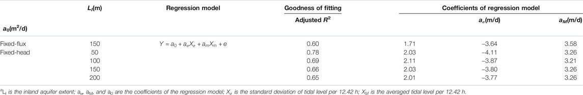
TABLE 2. Summary of regression results for submarine groundwater discharge (SGD)^a.

As expected, the response of the freshwater input, SM_SW and SM_USP, to the tides was delayed, which failed the regression model in Eq. 2 excluding the antecedent tidal conditions. Similar to Yu et al. (2019b), we defined the cumulative effect of antecedent multiconstituent tides (X_σ and X_M) in the regression models based on functional data analysis (Ramsay and Silverman, 2005). The cumulative effect was weighted in the form of the following convolution:

where DTL_i is the parametric regressor, i.e., the weighted antecedent tidal conditions combined in a cumulative fashion. The subscript i indicates the independent value. t is the present time and t − jΔt is the past time associated with the quantified antecedent tidal condition. The increment Δt of each time step was set to 12.42 h. X_i,t−jΔt is the variable at that past time. The subscript j indicates the past time period considered in the convolution, with the minimum and maximum values of n and m, respectively (set to 1 and 1,411 (two years), respectively). ${\mathit{\zeta }}_{\mathit{i}\mathrm{, }\mathit{j}}$ is a time-dependent weighting factor described by the following probability density function of the Gamma distribution:

where α_i and β_i are the shape and scale factors, respectively. The ratio α_i/β_i is the mean of the Gamma distribution, which indicates a tail of the distribution (a large α_i/β_i indicates a long tail). In addition, it reflects the overall contribution of the antecedent tidal conditions.

The freshwater inputs, SM_SW and SM_USP, were then quantified using a linear combination of $\mathit{DT}{\mathit{L}}_{\sigma }$ and $\mathit{DT}{\mathit{L}}_{\mathit{M}}$. Firstly, we tested the freshwater input using the regression model as follows:

For the cases with fixed-head inland boundaries, this regression model well captured the variation of the freshwater input for the cases with L_I = 200, 150, and 100 m (Table 3 and Supplementary Figures S3, S4; adjusted R² = 0.99, 0.99, 0.96, respectively). However, the regression result (adjusted R² = 0.65) for the case with L_I = 50 m was not as good as the other cases with longer inland aquifer extents. The freshwater input was affected by the lateral hydraulic gradient, which was a combination of the inland watertable and tidal level. Given a short inland aquifer extent, the lateral hydraulic gradient was more responsive to the tidal fluctuation as it took less time for tidal signals to propagate into the inland boundary. The signal reflection would thus moderate the inland freshwater input. In this way, the contribution of the antecedent tidal conditions would decrease, whereas that of the present tidal conditions would increase. This was clearly shown by α_i/β_i values for both $\mathit{DT}{\mathit{L}}_{\sigma }$ and $\mathit{DT}{\mathit{L}}_M$; for example, with L_I reduced from 200 to 150, 100, and 50 m, α_i/β_i for $\mathit{DT}{\mathit{L}}_{\sigma }$ decreased from 7.02 to 4.48, 2.38, and 1.44 days, respectively (Table 3 and Figure 8). As the regression model considered the antecedent tidal conditions only, it became poor for the cases with a short inland aquifer extent (e.g., that with L_I = 50 m).

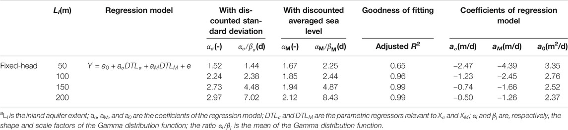
TABLE 3. Summary of regression results for inland freshwater input^a.

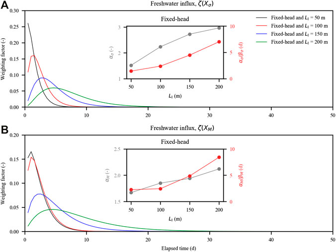
FIGURE 8. Probability density functions of inland freshwater input quantified with the antecedent tidal conditions on the aquifer: (A) time-dependent weighting factor for the standard deviation of tidal level (${\mathit{X}}_{\mathit{\sigma }}$) and (B) time-dependent weighting factor for the averaged tidal level (${\mathit{X}}_M$). The shape and mean parameters (α and α/β) of the Gamma distribution functions are given in the inserts.

Overall, α_i/β_i values for both $\mathit{DT}{\mathit{L}}_{\sigma }$ and $\mathit{DT}{\mathit{L}}_M$ were less than 10 days, suggesting that the recent tidal conditions were affected more on the freshwater input (Figure 8). Both the variation of α_i and α_i/β_i were monotonic. In particular, for all the cases with fixed-head inland boundaries, α_i values were larger than 1, suggesting that the maximum effect of the antecedent tidal conditions was delayed. With L_I reduced from 200 to 150, 100, and 50 m, ${\mathit{\alpha }}_{\sigma }$ for $\mathit{DT}{\mathit{L}}_{\sigma }$ decreased from 2.97 to 2.73, 2.24, and 1.52, respectively, whereas ${\mathit{\alpha }}_M$ for $\mathit{DT}{\mathit{L}}_M$ decreased from 8.43 to 4.87, 2.44, and 2.25 days, respectively. These trends were consistent with the tidal propagation; that is, it took less time for tidal signals to reach the inland boundary and moderate the freshwater input with the reduced L_I.

Secondly, we examined SM_SW. The regression model for the freshwater input (Eq. 5) well captured the variation of SM_SW for the cases with fixed-head inland boundaries (Table 4 and Supplementary Figures S5, S6) as well as that for the case with fixed-flux inland boundary (all the R² values were larger than 0.95). As L_I increased, both α_i and α_i/β_i values increased monotonously (Figure 9), suggesting that the effect of the antecedent tidal conditions on SM_SW was further delayed and prolonged as the inland aquifer extent increased.

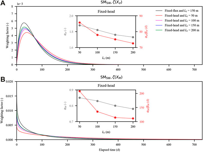
FIGURE 9. Probability density functions of the amount of salt stored in the saltwater wedge (SM_SW) quantified with the antecedent tidal conditions on the aquifer: (A) time-dependent weighting factor for the standard deviation of tidal level (${\mathit{X}}_{\mathit{\sigma }}$) and (B) time-dependent weighting factor for the averaged tidal level (${\mathit{X}}_M$). For the cases with fixed-head inland boundaries, the shape and mean parameters ($\mathit{\alpha }$ and $\mathit{\alpha }/\mathit{\beta }$) of the Gamma distribution functions are given in the inserts.

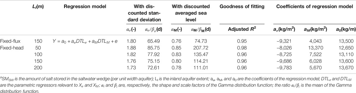
TABLE 4. Summary of regression results for SM_SW^a.

Finally, we checked SM_USP using the regression model given in Yu et al. (2019b) for the cases with fixed-flux inland boundaries.

where $\mathit{\omega }$ is the angular frequency related to the low-frequency of 6.50 × 10^–8 Hz (period of 178.1 d). ${\mathit{a}}_{\mathit{A}}$ and $\delta$ are the amplitude and the phase shift of this signal, respectively.

This regression model failed to capture the variation of SM_USP, particularly under the conditions of L_I = 50 and 100 m (Table 5 and Supplementary Figures S7, S8). The adjusted R² values for L_I = 50 and 100 m were, respectively, 0.23 and 0.47. This further demonstrated that the hydrodynamic process in the aquifers with fixed-head inland boundaries was more complicated than that with fixed-flux inland boundaries. As discussed earlier, in the former, the inland freshwater input was variable and affected by both the standard deviations and the averaged values of the antecedent tidal conditions. Therefore, we introduced the following new regression model with $\mathit{DT}{\mathit{L}}_M$ included to account for the varying freshwater input.

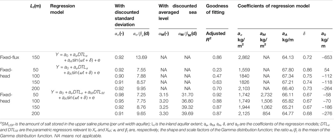
TABLE 5. Summary of regression results for SM_USP^a.

Then, the variation of SM_USP was well captured in both trend and magnitude for the cases with fixed-head inland boundaries (Table 5 and Supplementary Figures S9, S10). The fitted results were improved in the new regression model (adjusted R² of 0.23, 0.47, 0.63, and 0.70 for the old model (Eq. 6) in comparison with adjusted R² of 0.92, 0.88, 0.87, and 0.87 for the new model (Eq. 7). It is interesting that α_i/β_i values for both $\mathit{DT}{\mathit{L}}_{\sigma }$ and $\mathit{DT}{\mathit{L}}_M$ monotonically increased as L_I increased (Figure 10). However, α_i values for $\mathit{DT}{\mathit{L}}_{\sigma }$ and $\mathit{DT}{\mathit{L}}_M$ showed opposite trends. The former decreased but the latter increased. This suggests that as the inland aquifer extent increased, the effect of the mean tidal level on the USP was further delayed, whereas the effect of standard deviation was further enhanced. The USP developed in the seaside aquifer and was altered by both the fluctuation intensity of tides and the inland freshwater input. The opposite trends of the enhanced tidal effect and the reduced effect of the inland boundary on the USP are consistent with the previous studies (Werner et al., 2013; Robinson et al., 2018).

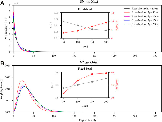
FIGURE 10. Probability density functions of the amount of salt stored in the upper saline plume (SM_USP) quantified with the antecedent tidal conditions on the aquifer: (A) time-dependent weighting factor for the standard deviation of tidal level (${\mathit{X}}_{\mathit{\sigma }}$) and (B) time-dependent weighting factor for the averaged tidal level (${\mathit{X}}_M$). For the cases with fixed-head inland boundaries, the shape and mean parameters ($\mathit{\alpha }$ and $\mathit{\alpha }/\mathit{\beta }$) of the Gamma distribution functions are given in the inserts.

Discussions

There are generally two types of inland boundary conditions for coastal unconfined aquifers: topography-controlled and constant freshwater discharge, to which the fixed-head and fixed-flux inland boundaries could be applied, respectively (Werner and Simmons, 2009). Given the similar freshwater input, the yearly averaged SGD and salinity distributions remained similar in the aquifers subjected to the multiconstituent tides. However, with the fixed-head inland boundary, the multiconstituent tides led to more remarkable fluctuations of the USP and SW, in comparison with those for the case with fixed-flux inland boundary. This reflects intensive mixing between freshwater and seawater, which was shown to intensify as the inland aquifer extent decreased. As chemical compositions of seaward seawater and land-sourced fresh groundwater are apparently different, these enhanced mixing between freshwater and seawater would favor biogeochemical reactions in coastal aquifers (Robinson et al., 2018).

With the fixed-head inland boundaries, the lateral hydraulic gradient varied in response to the multiconstituent tides. This led to a varying inland freshwater input, which was more remarkable as the inland aquifer extent decreased. However, the SGD, as the total water efflux, kept a similar fluctuation trend for all the cases and was not significantly altered by the inland aquifer extent. Based on the principle of mass conservation, it is expected that the varying inland freshwater input would moderate the storage of both the freshwater and land-sourced chemicals stored in the aquifer.

The spectrum analysis of the SGD and SM_SW showed that the importance of different signals was similar for the aquifers with fixed-head or fixed-flux inland boundaries. The spectrum of freshwater input demonstrated the significant effect of low-frequency signal (365-day period) in the fixed-head inland aquifers and its influence increased as the inland aquifer extent increased. This suggests that the signal of the year-long period in the tidal series was enhanced in the inland freshwater input. The influence of this signal also increased with the increased inland aquifer extent for the size of USP in the aquifers with fixed-head inland boundaries. Consistently, the 365-day period signal did not appear in the spectrum of SM_USP for the aquifer with fixed-flux inland boundary. These results were overall consistent with previous studies that coastal aquifers with fixed-head inland boundaries are more responsive to changes to ocean boundary conditions as groundwater discharge and salt distributions can be easily changed (Werner and Simmons, 2009; Michael et al., 2013). Our results further highlighted the importance of low-frequency tidal fluctuations. Not only the SW but also the USP was affected by low-frequency signals. In particular, the USP was affected more by low-frequency signals as the inland aquifer extent increased. At a longer-time scale, the location of the fixed-head inland boundary in a natural aquifer depends on the local topography and mean sea level. A relative sea-level rise, as a combination of the two, is expected to reduce the inland aquifer extent. In this way, the high-frequency tidal signals would play a more important role in affecting salinity distributions (both the SW and USP).

SGD is extensively recognized for delivering considerable land-sourced chemicals to the sea and thus affects marine ecosystems such as inducing coastal eutrophication. Salinity distributions in aquifers affect terrestrial ecosystems and fresh groundwater use in coastal areas. Based on our results, the response of the SGD to multiconstituent tides is mostly instantaneous. This suggests that an intensified oceanic forcing condition may instantaneously lead to large input of chemicals to the sea. The variations of the SW and USP are insensitive to the present tidal conditions but related to the antecedent tidal conditions. Oceanic forcing conditions would affect the salinity distributions in aquifers in a prolonged fashion. This suggests that the management of coastal groundwater resources such as control of seawater intrusion could carefully consider antecedent oceanic forcing conditions and long-lasting impacts of human activities (e.g., groundwater extraction and recharge). The regression models presented in this study provide a way for predicting salinity distributions in coastal aquifers under different scenarios and would help guide decision-making.

Conclusions

This article has examined the SGD and salinity distributions in coastal aquifers with fixed-head inland boundaries and subjected to the influence of multiconstituent tides. The numerical simulations with different inland aquifer extents represented the typical topography-controlled unconfined coastal aquifers. The following conclusions can be drawn:

• Given a similar yearly averaged freshwater input, the SGD responded instantaneously to the multiconstituent tides. The effect of the inland aquifer extent on SGD was minor. However, the USP and SW fluctuations were enhanced as the inland aquifer extent decreased.

• Inland freshwater input was affected by the combination of the inland aquifer extent and multiconstituent tides. Filtering effect of the aquifer on the high-frequency tidal signals was weakened as the inland aquifer extent decreased and that led to enhanced fluctuations of the freshwater input. The varying freshwater input in turn affected remarkably the salinity distributions in the aquifer.

• The regression modeling approaches developed in Yu et al. (2019b) were shown to be able to quantify the variation of the SGD and SW but did not work well for the USP. The cumulative influence of the antecedent lateral hydraulic gradients (as a combination of inland watertable and tidal level) was further included in the new regression model for the USP.

In natural systems, the inland condition is more complex than that of either fixed-head or fixed-flux inland boundary as the inland freshwater input is commonly irregular in response to local rainfall, evapotranspiration, and anthropic groundwater use. While our regression models well captured the SGD and salinity distributions in both aquifers with fixed-head and fixed-flux inland boundaries, they remain to be tested for real aquifer systems. It is worth noting that most natural aquifers are also affected by high-frequency waves and episodic rainfall. All these forcing factors would affect SGD process and salinity distributions in a prolonged fashion (Xin et al., 2014; Yu et al., 2017). Long-term investigations are necessary for applying our regression models in real coastal aquifers. With available long-term datasets, possible quantitative analysis on the interaction among these forcing factors would help to uncover complex SGD process and salinity distributions. Nevertheless, the present study has provided guidance for future research, including field investigations that aim to establish the principle link of SGD and salinity distributions to hydrological forcing factors.

Data Availability Statement

The raw data supporting the conclusions of this article will be made available by the authors, without undue reservation.

Author Contributions

XY: methodology, formal analysis, data curation, conceptualization, and writing the original draft. PX: conceptualization, methodology, supervision, and writing, review and editing. CS: methodology and supervision. LL: methodology and writing, review and editing.

Funding

This work was supported by the National Natural Science Foundation of China (U2040204 and 41807178) and the Fundamental Research Funds for the Central Universities (2019B80414 and 2019B12314).

Conflict of Interest

The authors declare that the research was conducted in the absence of any commercial or financial relationships that could be construed as a potential conflict of interest.

Supplementary Material

The Supplementary Material for this article can be found online at: https://www.frontiersin.org/articles/10.3389/fenvs.2020.599041/full#supplementary-material

Abbreviations

SGD, submarine groundwater discharge; USP, upper saline plume; SW, saltwater wedge; H_f, inland watertable elevation; H_I, inland aquifer thickness; H_S, seaward aquifer thickness; L_I, inland aquifer extent; L_S, seaward aquifer extent; SM_SW, amount of salt stored in saltwater wedge; SM_USP, amount of salt stored in upper saline plume; M₂, principal lunar semidiurnal tidal constituent; S₂, principal solar semidiurnal tidal constituent; K₁, lunisolar declinational diurnal tidal constituent; N₂, larger lunar elliptic semidiurnal tidal constituent

References

Abarca, E., Karam, H., Hemond, H. F., and Harvey, C. F. (2013). Transient groundwater dynamics in a coastal aquifer: the effects of tides, the lunar cycle, and the beach profile. Water Resour. Res. 49 (5), 2473–2488. doi:10.1002/wrcr.20075
Ataie-Ashtiani, B., Volker, R. E., and Lockington, D. A. (1999). Tidal effects on sea water intrusion in unconfined aquifers. J. Hydrol. 216 (1–2), 17–31. doi:10.1016/S0022-1694(98)00275-3
Boufadel, M. C. (2000). A mechanistic study of nonlinear solute transport in a groundwater-surface water system under steady state and transient hydraulic conditions. Water Resour. Res. 36 (9), 2549–2565. doi:10.1029/2000wr900159
Buquet, D., Sirieix, C., Anschutz, P., Malaurent, P., Charbonnier, C., Naessens, F., et al. (2016). Shape of the shallow aquifer at the fresh water–sea water interface on a high-energy sandy beach. Estuarine. Coast. Shelf Sci. 179, 79–89. doi:10.1016/j.ecss.2015.08.019
Carsel, R. F., and Parrish, R. S. (1988). Developing joint probability distributions of soil water retention characteristics. Water Resour. Res. 24 (5), 755–769. doi:10.1029/WR024i005p00755
Evans, T. B., and Wilson, A. M. (2016). Groundwater transport and the freshwater–saltwater interface below sandy beaches. J. Hydrol. 538, 563–573. doi:10.1016/j.jhydrol.2016.04.014
Geng, X., and Boufadel, M. C. (2015). Impacts of evaporation on subsurface flow and salt accumulation in a tidally influenced beach. Water Resour. Res. 51 (7), 5547–5565. doi:10.1002/2015WR016886
Geng, X., and Boufadel, M. C. (2017). Spectral responses of gravel beaches to tidal signals. Sci. Rep. 7 (1), 40770. doi:10.1038/srep40770 |
Heiss, J. W., and Michael, H. A. (2014). Saltwater-freshwater mixing dynamics in a sandy beach aquifer over tidal, spring-neap, and seasonal cycles. Water Resour. Res. 50 (8), 6747–6766. doi:10.1002/2014WR015574
Hunt, A. G., Skinner, T. E., Ewing, R. P., and Ghanbarian-Alavijeh, B. (2011). Dispersion of solutes in porous media. Eur. Phys. J. B 80 (4), 411–432. doi:10.1140/epjb/e2011-10805-y
Kuan, W. K., Jin, G., Xin, P., Robinson, C., Gibbes, B., and Li, L. (2012). Tidal influence on seawater intrusion in unconfined coastal aquifers. Water Resour. Res. 48 (2), W02502. doi:10.1029/2011WR010678
Kuan, W. K., Xin, P., Jin, G., Robinson, C. E., Gibbes, B., and Li, L. (2019). Combined effect of tides and varying inland groundwater input on flow and salinity distribution in unconfined coastal aquifers. Water Resour. Res. 55 (11), 8864–8880. doi:10.1029/2018WR024492
Levanon, E., Shalev, E., Yechieli, Y., and Gvirtzman, H. (2016). Fluctuations of fresh-saline water interface and of water table induced by sea tides in unconfined aquifers. Adv. Water Resour 96, 34–42. doi:10.1016/j.advwatres.2016.06.013
Levanon, E., Yechieli, Y., Gvirtzman, H., and Shalev, E. (2017). Tide-induced fluctuations of salinity and groundwater level in unconfined aquifers – field measurements and numerical model. J. Hydrol 551, 665–675. doi:10.1016/j.jhydrol.2016.12.045
Li, L., Barry, D. A., and Pattiaratchi, C. B. (1997). Numerical modelling of tide-induced beach water table fluctuations. Coast. Eng. 30 (1–2), 105–123. doi:10.1016/S0378-3839(96)00038-5
Li, L., Barry, D. A., Stagnitti, F., Parlange, J-Y., and Jeng, D-S. (2000). Beach water table fluctuations due to spring–neap tides: moving boundary effects. Adv. Water Resour. 23 (8), 817–824. doi:10.1016/S0309-1708(00)00017-8
Mao, X., Enot, P., Barry, D. A., Li, L., Binley, A., and Jeng, D. S. (2006). Tidal influence on behaviour of a coastal aquifer adjacent to a low-relief estuary. J. Hydrol 327 (1–2), 110–127. doi:10.1016/j.jhydrol.2005.11.030
Michael, H. A., Mulligan, A. E., and Harvey, C. F. (2005). Seasonal oscillations in water exchange between aquifers and the coastal ocean. Nature 436 (7054), 1145–1148. doi:10.1038/nature03935 |
Michael, H. A., Russoniello, C. J., and Byron, L. A. (2013). Global assessment of vulnerability to sea-level rise in topography-limited and recharge-limited coastal groundwater systems. Water Resour. Res. 49 (4), 2228–2240. doi:10.1002/wrcr.20213
Pawlowicz, R., Beardsley, B., and Lentz, S. (2002). Classical tidal harmonic analysis including error estimates in MATLAB using T_TIDE. Comput. Geosci 28 (8), 929–937. doi:10.1016/S0098-3004(02)00013-4
Robinson, C., Gibbes, B., Carey, H., and Li, L. (2007a). Salt-freshwater dynamics in a subterranean estuary over a spring-neap tidal cycle. J. Geophys. Res. 112 (C9), C09007. doi:10.1029/2006JC003888
Robinson, C., Li, L., and Barry, D. A. (2007b). Effect of tidal forcing on a subterranean estuary. Adv. Water Resour 30 (4), 851–865. doi:10.1016/j.advwatres.2006.07.006
Robinson, C., Li, L., and Prommer, H. (2007c). Tide-induced recirculation across the aquifer-ocean interface. Water Resour. Res. 43 (7), W07428. doi:10.1029/2006WR005679
Robinson, C., Gibbes, B., and Li, L. (2006). Driving mechanisms for groundwater flow and salt transport in a subterranean estuary. Geophys. Res. Lett. 33 (3), L03402. doi:10.1029/2005GL025247
Robinson, C. E., Xin, P., Santos, I. R., Charette, M. A., Li, L., and Barry, D. A. (2018). Groundwater dynamics in subterranean estuaries of coastal unconfined aquifers: controls on submarine groundwater discharge and chemical inputs to the ocean. Adv. Water Resour. 115, 315–331. doi:10.1016/j.advwatres.2017.10.041
Sawyer, A. H., David, C. H., and Famiglietti, J. S. (2016). Continental patterns of submarine groundwater discharge reveal coastal vulnerabilities. Science. 353 (6300), 705–707. doi:10.1126/science.aag1058 |
Shen, C., Zhang, C., Kong, J., Xin, P., Lu, C., Zhao, Z., et al. (2019). Solute transport influenced by unstable flow in beach aquifers. Adv. Water Resour 125, 68–81. doi:10.1016/j.advwatres.2019.01.009
Van Genuchten, M. T. (1980). A closed-form equation for predicting the hydraulic conductivity of unsaturated soils. Soil Sci. Soc. Am. J. 44 (5), 892–898. doi:10.2136/sssaj1980.03615995004400050002x
Voss, C. I., and Provost, A. M. (2010). SUTRA, A model for saturated-unsaturated variable-density ground-water flow with solute or energy transport. Available at: http://pubs.er.usgs.gov/publication/wri024231.
Werner, A. D., Bakker, M., Post, V. E. A., Vandenbohede, A., Lu, C., Ataie-Ashtiani, B., et al. (2013). Seawater intrusion processes, investigation and management: recent advances and future challenges. Adv. Water Resour 51, 3–26. doi:10.1016/j.advwatres.2012.03.004
Werner, A. D., and Simmons, C. T. (2009). Impact of sea-level rise on sea water intrusion in coastal aquifers. Ground Water 47 (2), 197–204. doi:10.1111/j.1745-6584.2008.00535.x |
Xin, P., Wang, S. S. J., Robinson, C., Li, L., Wang, Y-G., and Barry, D. A. (2014). Memory of past random wave conditions in submarine groundwater discharge. Geophys. Res. Lett. 41 (7), 2401–2410. doi:10.1002/2014GL059617
Yu, X., Xin, P., Lu, C., Robinson, C., Li, L., and Barry, D. A. (2017). Effects of episodic rainfall on a subterranean estuary. Water Resour. Res. 53 (7), 5774–5787. doi:10.1002/2017WR020809
Yu, X., Xin, P., and Lu, C. (2019a). Seawater intrusion and retreat in tidally-affected unconfined aquifers: laboratory experiments and numerical simulations. Adv. Water Resour. 132, 103393. doi:10.1016/j.advwatres.2019.103393
Keywords: submarine groundwater discharge, seawater intrusion, coastal aquifer, functional data analysis, numerical modeling
Citation: Yu X, Xin P, Shen C and Li L (2021) Effects of Multiconstituent Tides on a Subterranean Estuary With Fixed-Head Inland Boundary. Front. Environ. Sci. 8:599041. doi: 10.3389/fenvs.2020.599041
Received: 28 August 2020; Accepted: 14 December 2020;
Published: 19 January 2021.
Edited by:
Carlos Rocha, Trinity College Dublin, IrelandReviewed by:
Anupma Sharma, National Institute of Hydrology (Roorkee), IndiaPedro Giovâni Da Silva, Federal University of Minas Gerais, Brazil
Copyright © 2021 Yu, Xin, Shen and Li. This is an open-access article distributed under the terms of the Creative Commons Attribution License (CC BY). The use, distribution or reproduction in other forums is permitted, provided the original author(s) and the copyright owner(s) are credited and that the original publication in this journal is cited, in accordance with accepted academic practice. No use, distribution or reproduction is permitted which does not comply with these terms.
*Correspondence: Pei Xin, pei.xin@outlook.com