Machine Learning Using Rapidity-Mass Matrices for Event Classification Problems in HEP


Argonne National Laboratory, HEP Division, 9700 S. Cass Avenue, Argonne, IL 60439, USA
Universe 2021, 7(1), 19; https://doi.org/10.3390/universe7010019
Submission received: 17 December 2020
/
Revised: 13 January 2021
/
Accepted: 16 January 2021
/
Published: 19 January 2021
(This article belongs to the Special Issue Enhancing Sensitivity to Physics beyond the Standard Model and Detector Performance Monitoring in HEP Experiments with Machine Learning)
Abstract
:In this work, supervised artificial neural networks (ANN) with rapidity–mass matrix (RMM) inputs are studied using several Monte Carlo event samples for various collision processes. The study shows the usability of this approach for general event classification problems. The proposed standardization of the ANN feature space can simplify searches for signatures of new physics at the Large Hadron Collider (LHC) when using machine learning techniques. In particular, we illustrate how to improve signal-over-background ratios in the search for new physics, how to filter out Standard Model events for model-agnostic searches, and how to separate gluon and quark jets for Standard Model measurements.
1. Introduction
Transformations of lists with four-momenta particles produced in collision events into rapidity–mass matrices (RMM) [1] that encapsulate information on the single and two-particle densities of identified particles and jets can lead to a systematic approach to defining input variables for various artificial neural networks (ANNs) used in particle physics. By construction, the RMMs are expected to be sensitive to a wide range of popular event signatures of the Standard Model (SM), and thus can be used for various searches for new signatures beyond the Standard Model (BSM).
It is important to remember that the RMM matrix is constructed from all reconstructed objects (leptons, photons, missing transverse energies, and jets). The size of this 2D matrix is fixed by the maximum number of expected objects and the number of possible object types. The diagonal elements of the RMM represent transverse momenta of all objects, the upper-right elements are invariant masses of each two-particle combination, and the lower-left cells reflect rapidity differences. Event signatures with missing transverse energies and Lorentz factors are also conveniently included. A RMM matrix for two distinct objects is illustrated in the Appendix A. The definition of the RMM is mainly driven by the requirement of small correlations between RMM cells. The usefulness of the RMM formalism has been demonstrated in [1] using a toy example of background reduction for charged Higgs searches.
In the past, separate variables of the RMM have already been used for the “feature” space for machine learning applications in particle collisions. A recent example of a machine learning approach that uses the numbers of jets, jet transverse momenta, and rapidities as inputs for neural network algorithms can be found in [2]. Unlike a handcrafted set of variables, the RMM represents a well-defined organization principle for creating unique “fingerprints” of collision events suitable for a large variety of event types and ANN architectures due to the unambiguous mapping of a broad number of experimental signatures to the ANN nodes. Therefore, a time-consuming determination of the feature space for every physics topic, as well as preparations of this feature space (i.e., re-scaling, normalization, de-correlation etc.) for machine learning, may not be required as RMMs already satisfy the most standard requirements for supervised machine learning algorithms.
The results presented in this paper confirm that the standard RMM transformation is a convenient choice for general event classification problems using supervised machine learning. In particular, we illustrate that repetitive and tedious tasks of feature-space engineering to identify ANN inputs for different event categories can be fully or partially automated. This paper illustrates a few use cases of this technique. In particular, we show how to improve signal-over-background ratios in searches for BSM physics (Section 3), how to filter out SM events for model-agnostic searches (Section 4), and how to separate gluon and quark jets for SM measurements (Section 5).
2. Event Classification with RMM
In this section, we will illustrate that the feature space in the form of the standard RMM can conveniently be applied for event-classification problems for a broad class of collision processes simulated with the help of Monte Carlo (MC) event generators.
This analysis is based on the Pythia8 MC model [3,4] for the generation of -collision events at the TeV center of mass energy. The NNPDF 2.3 LO [5] parton density function from the LHAPDF library [6] was used. The following five collision processes were simulated: (1) multijet events from quantum chromodynamics (QCD) processes events, (2) Standard Model (SM) Higgs production, (3) production, (4) double-boson production and (5) a charged Higgs boson () process using the diagram for models with two (or more) Higgs doublets [7]. A minimum value of 50 GeV for generated invariant masses of the system was set. For each event category, all available sub-processes were simulated at leading-order QCD with parton showers and hadronization. Stable particles with a lifetime of more than seconds were considered, while neutrinos were excluded from consideration. All decays of top quarks, H and vector bosons were allowed. The files with the events were archived in the HepSim repository [8].
Jets, isolated electrons, muons, and photons were reconstructed using the procedure described in [1]. Jets were constructed with the anti- algorithm [9] as implemented in the FastJet package [10] using a distance parameter of . The minimum transverse energy of all jets was 40 GeV in the pseudorapidity range of . Jets were classified as light-flavor and as b-jets, which were identified by matching the momenta of b-quarks with reconstructed jets and requiring that the total momenta of b-quarks should be larger than 50% of the total jet energy. The b-jet fake rate was also included assuming that it increased from 1% to 6% at the largest [11].
Muons, electrons, and photons were reconstructed from Pythia8 truth-level information after applying isolation criteria [1]. These particles were reconstructed after applying an isolation radius of 0.1 in the space around the lepton direction. A lepton was considered to be isolated if it carried more than of the cone energy. To simulate the electron fake rate, we replaced jets with the number of constituents less than 10 with the electron ID using probability. In the case of muons, we used a misidentification rate; i.e., replacing jets with the muon ID in of cases. The fake rates considered here are representative and, generally, are the upper limits for the rates discussed in [12]. The minimum value of the transverse momentum of all leptons and photons was 20 GeV. The missing transverse energy is recorded above 50 GeV.
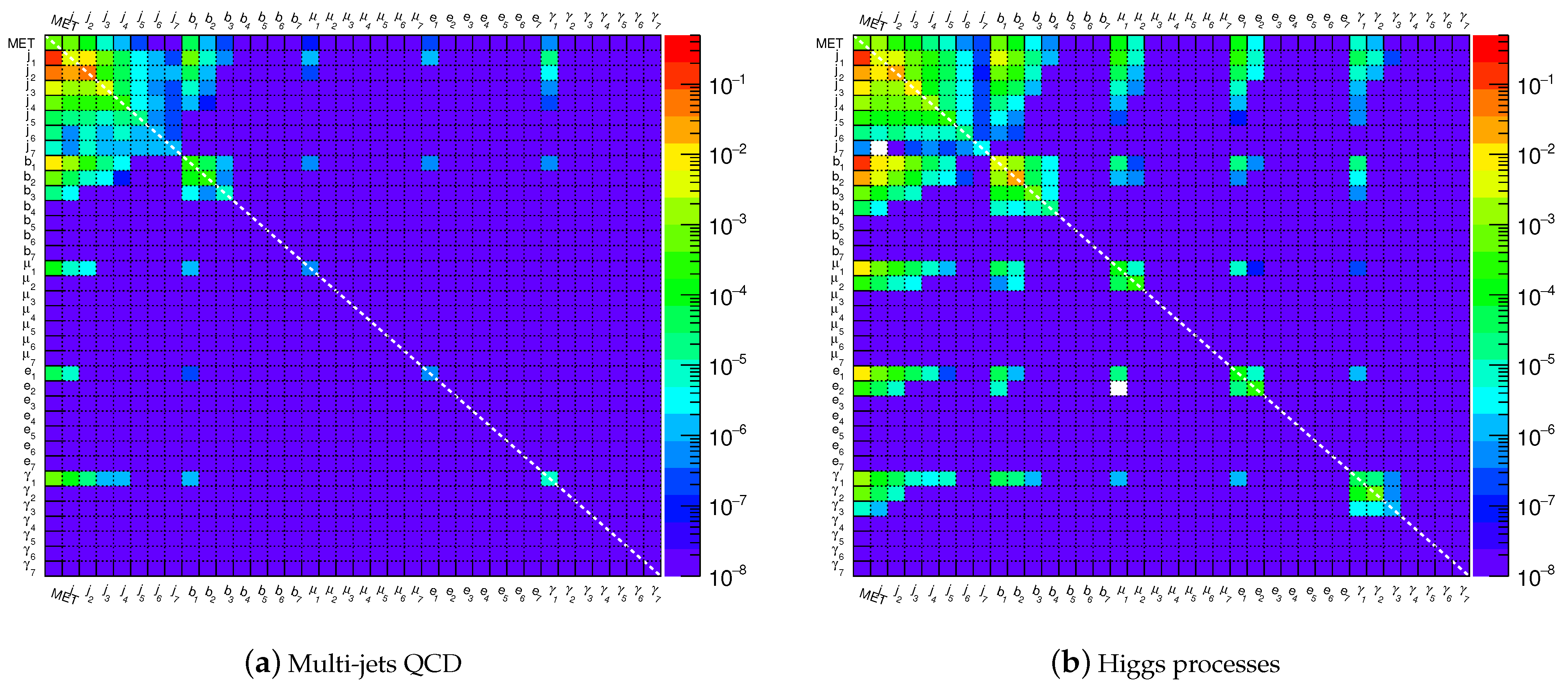
To prepare the event samples for an ANN event classification, the events were transformed to the RMMs with five types () of reconstructed objects: jets (j), b-jets (b), muons (), electrons (e), and photons (). Up to seven particles per type were considered (), leading to the so-called T5N7 topology for the RMM inputs. This transformation created RMMs with a size of 36 × 36. Only nonzero elements of such sparse matrices (and their indexes) were stored for further processing. Figure 1 shows the RMMs for multijet QCD events and the SM Higgs production after averaging the RMMs over 100,000 simulated collision events. As expected, the differences between these two processes, as seen in Figure 1, are due to the decays of the SM Higgs boson.
To illustrate the event-classification capabilities using the common RMM input space for different event categories, we have chosen to use a simple shallow (with one hidden layer) backpropagation ANN from the FANN package [13]. If the classification works for such a simple and well-established algorithm, this will build a baseline for the future exploration of more complex machine-learning techniques. The sigmoid activation function was used for all ANN nodes. No re-scaling of the input values was applied since the range is fixed by the RMM definition. The ANN had 1296 input nodes mapped to the cells of the RMM, after converting the matrices to one-dimensional arrays. A single hidden layer had 200 nodes, while the output layer had five nodes, , , corresponding to five types of events. Each node of the output layer was assigned the value 0 (“false”) or 1 (“true”) during the training process. The QCD multijet events correspond to (with all other values being zero), the Standard Model Higgs events correspond to (with all other values being zero) and so on. According to this definition, the value of the output node corresponds to the probability for identification of a given process.
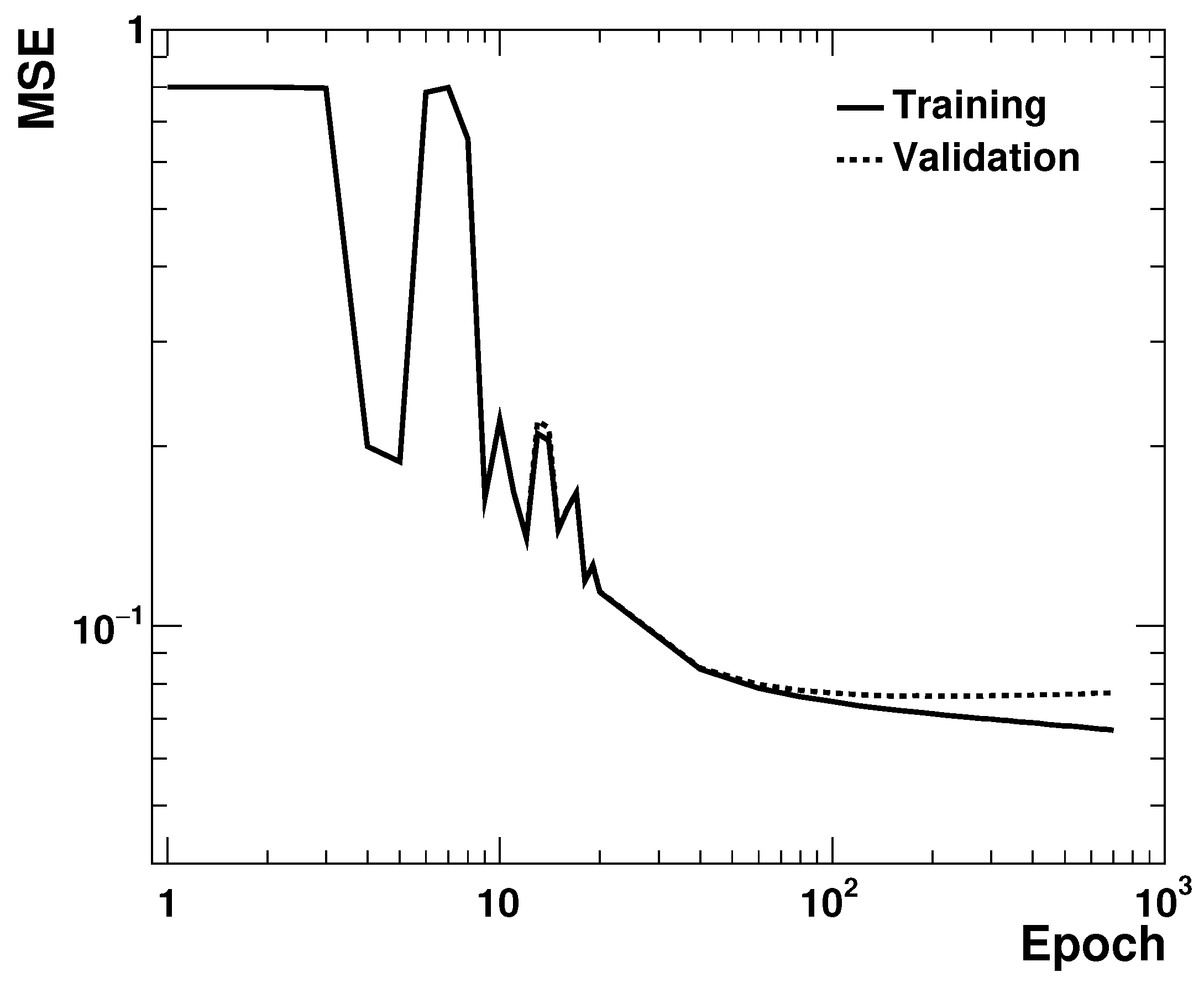
The goal of the ANN training was to reproduce the five values of the output layer for the known event types. During the training, a second (“validation”) data sample was used, which was constructed from 20,000 RMMs for each event type. Figure 2 shows the mean squared error (MSE) as a function of the number of epochs during the training procedure. The dashed line shows the MSE for the independent validation sample. As expected for a well-behaved training procedure, MSE values decreased as the number of epochs increased. The effect of over-training was observed after 100 epochs, after which the validation dataset did not show a decreasing trend for the MSE errors. Therefore, the training was terminated after 100 epochs. After the training, the MSE decreased from 0.8 to 0.065 (the value of 0.4 corresponded to the case when no training was possible). It is quite remarkable that the training based on the RMM converged after a relatively small number of epochs1.
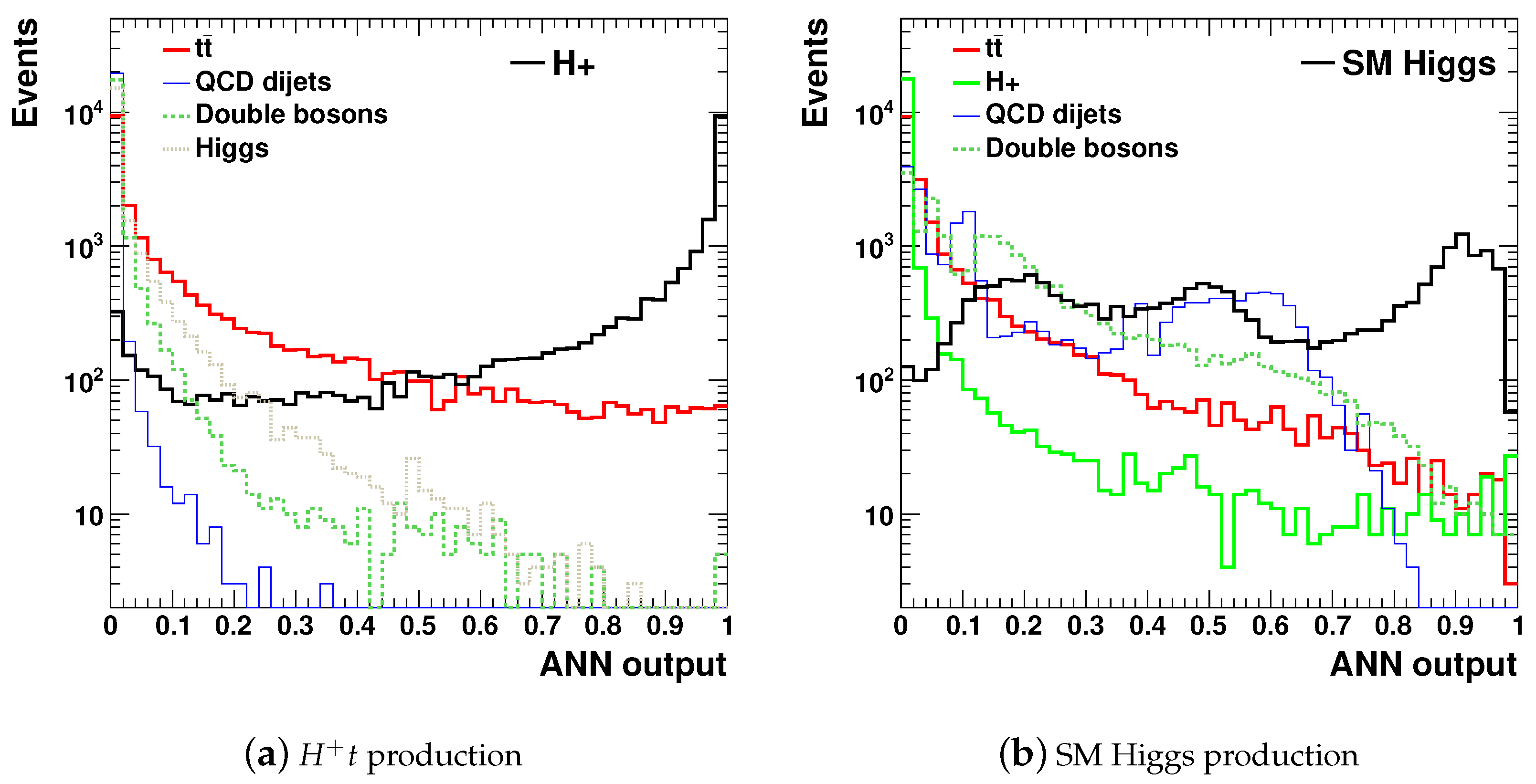
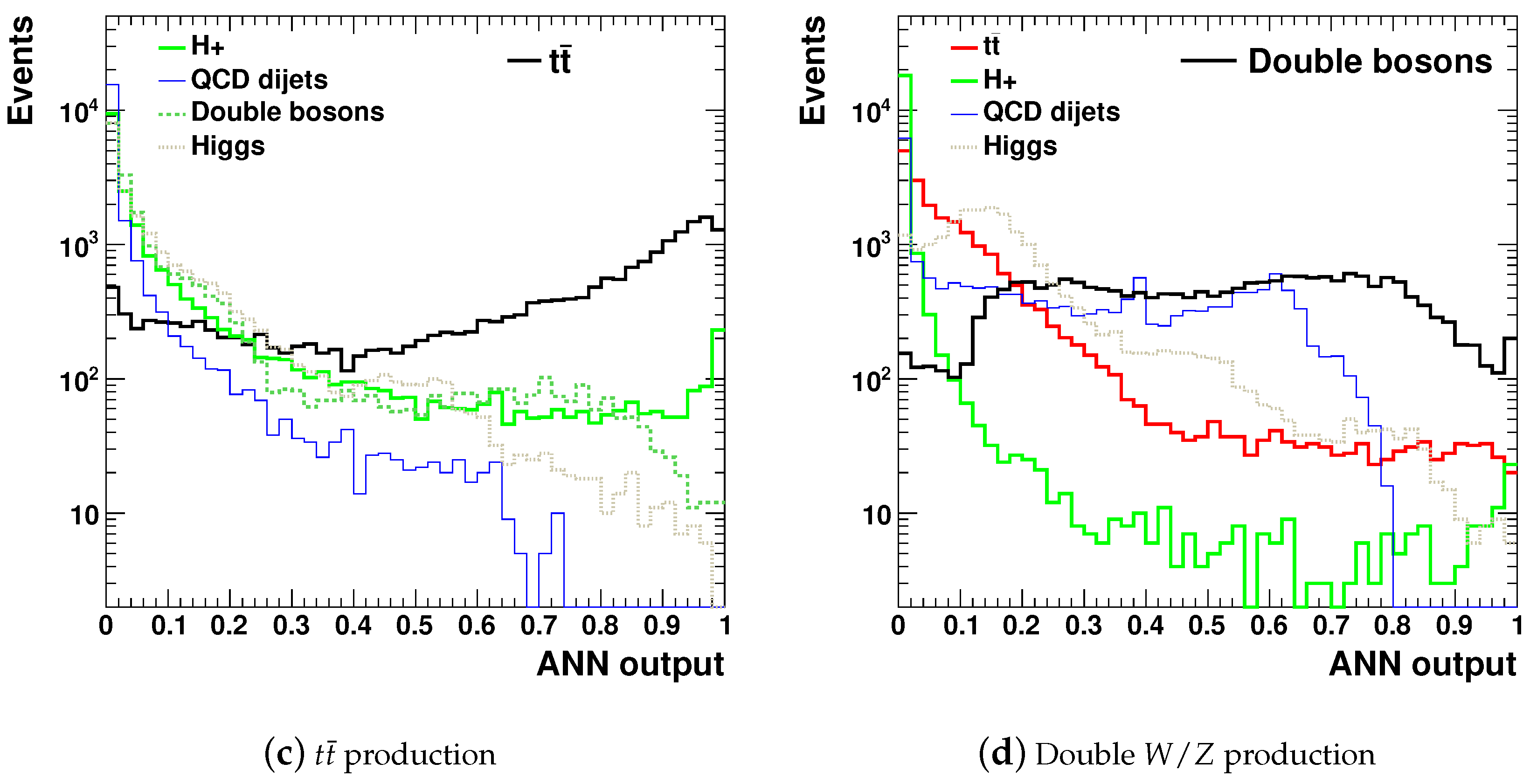
The trained ANN was applied to a third independent sample with 100,000 RMMs from all five event categories. Figure 3 shows the values of the output layer of the trained network for the charged Higgs, SM Higgs, , and double production. The ANN output values for multijet QCD events are not shown to avoid redundancy in presenting the results. As expected for robust event identification, peaks near 1 are observed for the four considered process types.
The success of the ANN training was evaluated in terms of the purity of identified events at a given value on the ANN output node. This purity was defined as a ratio of the number of events passed a cut of 0.8 on the ANN output score for a given input, divided by the total number of accepted events (regardless of their origin) above this cut. The purity of events for , and SM Higgs was close to 90%, while the purity for the reconstruction of the double-boson process was 80%. The dominant contributor to the background in the latter case was the process.
3. Background Reduction for BSM Searches
One immediate application of the RMM is to reduce a large rate of background events from SM events and to increase signal-over-background (S/B) ratios for exotic processes. As discussed before, the RMMs can be used as generic inputs without handcrafting variables for each SM and BSM event type. As a result, a single neural network with a unified input feature space and multiple output nodes can be used.
In this example, we use MC events that, typically, have at least one lepton and two hadronic jets per event. The jets can be associated with decays of heavy resonances. The Pythia Monte Carlo model was used to simulate the following event samples.
- Standard Model W + jet, Z + jets, Higgs, , and single-top events combined according to their corresponding cross sections. This event sample has a large rate of events with leptons and jets, thus it should represent the major background for BSM models predicting high rates of leptons and jets;
- events, as discussed in Section 2;
- events from the Sequential Standard Model (SSM) [14]. In this BSM model, , where W decays leptonically into and the heavy decays hadronically into two jets;
- A -model. It is a variation of technicolor models [15] where a resonance, , decays through the s-channel to the SM W boson and a technipion, , where the W and subsequently decay into leptons and jets, respectively;
- A model with heavy from the process in a simplified Dark Matter model [16] with the W production, where a decays to two jets, while W decays leptonically into .
In order to create a SM “background” sample for the BSM models considered above, the first and the second event samples were combined using the cross-sections predicted by Pythia. The event rates of the latter four BSM models, defined as , SSM, and (DM), are also predicted by this MC generator, with the settings given in [8]. The and SSM models and their settings were also discussed in [17]. The BSM models were generated assuming 1, 2, and 3 TeV masses for the , and heavy particles. About 20,000 events were generated for the BSM models, and about 2 million events were generated for the SM processes. For each event category, all available sub-processes were simulated at leading-order QCD with parton showers and hadronization. Jets, b-jets, isolated electrons and muons and photons were reconstructed using truth-level information as described in Section 2. The minimum transverse momentum of all leptons was set to 30 GeV, while the minimum transverse momentum of jets was 20 GeV.
Note that all six processes considered above have similar final states since they contain a lepton and a few jets. Therefore, the separation of such events is somewhat more challenging for the RMM–ANN approach, compared to the processes discussed in Section 2, which had distinct final states (QCD dijet events were not preselected by requiring an identified lepton).
Similar to Section 2, the generated collision events were transformed to the RMM representation with five types () of reconstructed objects. The capacity of the matrix was increased from to in order to allow contributions from particles (jets) with small transverse momenta. This “T5N10” input configuration led to sparse matrices with a size of .
The T5N10 RMM matrices were used as the input for a shallow back-propogation neural network with input nodes. The ANN had a similar structure as that discussed in Section 2: A single hidden layer had 200 nodes, while the output layer had six nodes, , , corresponding to six types of the considered events. Each node of the output layer has the value 0 (“true”) or 1 (“false”). The ANN contained 2809 neurons with 521,606 connections. The training was stopped after 200 epochs after using an independent validation sample. The CPU time required for the ANN training was similar to that discussed in the previous section.
For each MC sample, dijet invariant masses, , were reconstructed by combining the two leading jets with the highest values of jet transverse momentum. was the primary observable variable for which the impact of the ANN training procedure was tested. To avoid biases for the distribution after the application of the ANN, all cells associated with the variables were removed from the ANN training. The following cell positions were set to contain zero values:
- (1, 1), which corresponds to the energy of a leading jet;
- (1 + N, 1 + N), which corresponds to the energy of a leading b-jet;
- (2, 1), which corresponds to the of two leading light-flavor jets;
- (1 + N, 2 + N), which corresponds to the of two leading b-jets;
- (1 + N, 2), which corresponds to the of one leading light-flavor jet and b-jet.
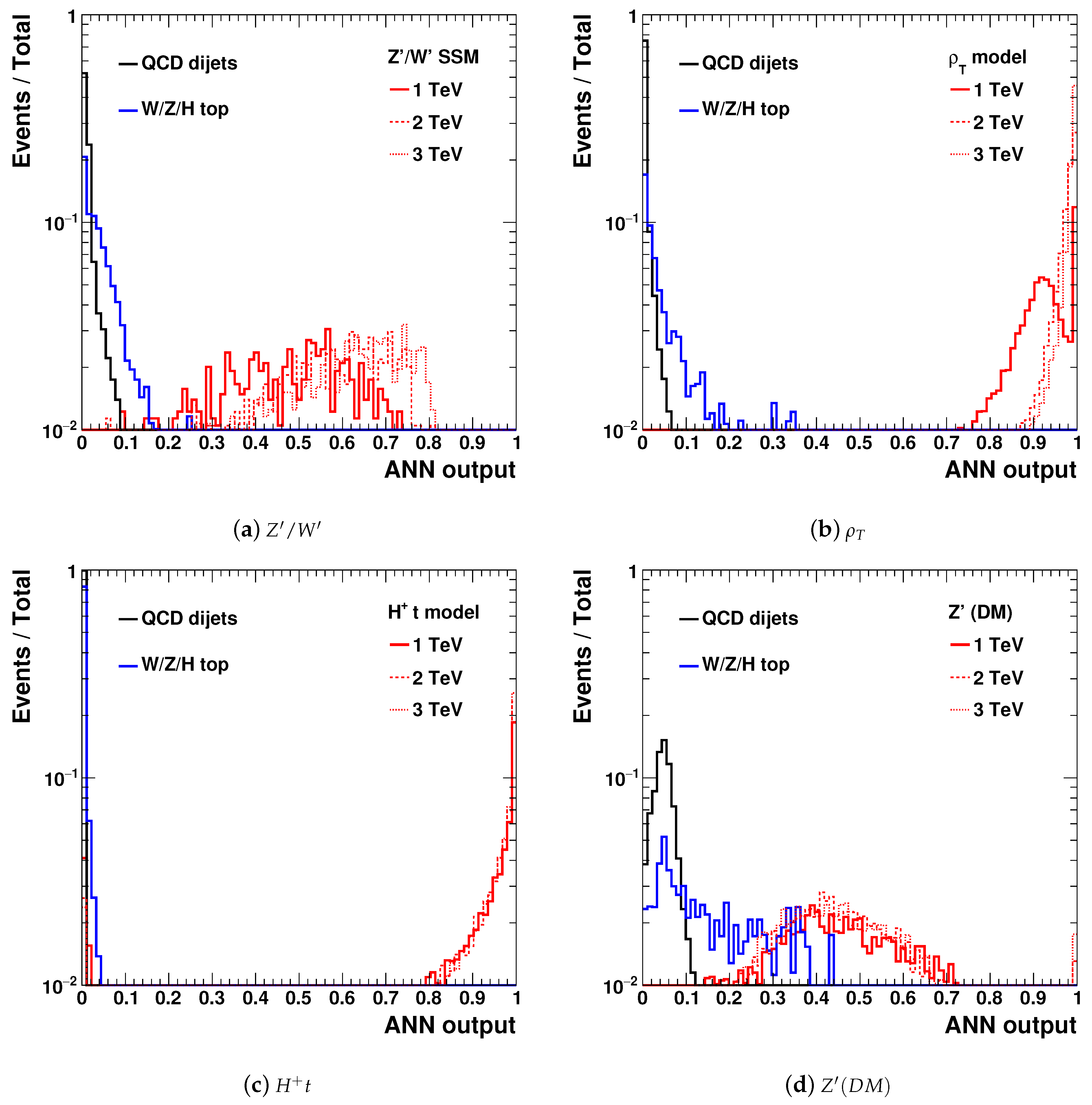
Figure 4 shows the values of the output neurons that correspond to the four BSM models, together with the values for the SM background processes. As expected, the ANN outputs were close to zero for the SM background, indicating a good separation power between the BSM models and the SM processes in the output space of the ANN. According to this figure, background events could be efficiently removed after requiring the output values on the BSM nodes above 0.2.
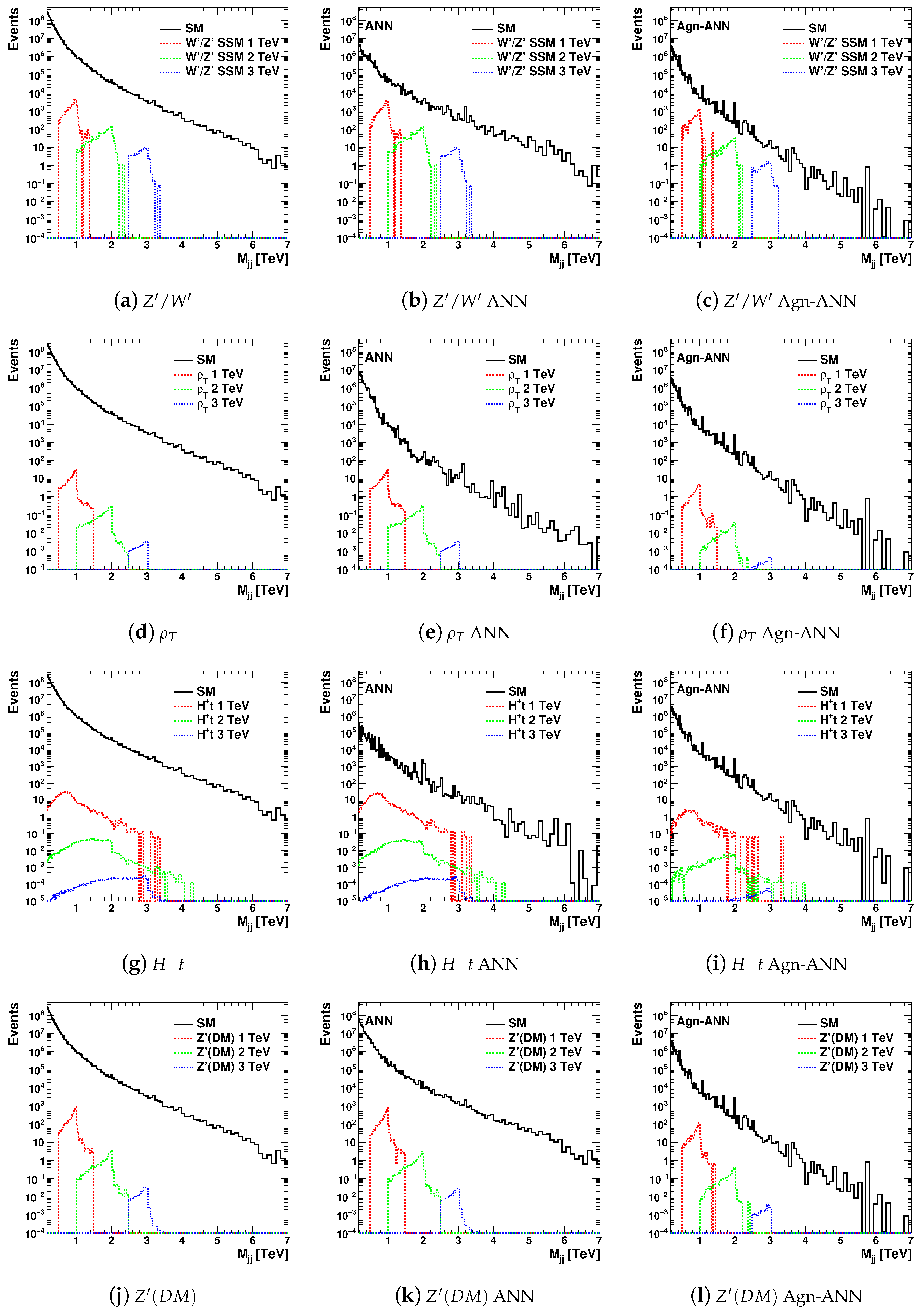
Figure 5 show the distributions for the background and signal events for collisions at = 13 TeV using an integrated luminosity of 150 fb. The SM background was a sum of the dijet QCD sample and the sample that included SM and top events. The BSM signals discussed above are shown for three representative masses, 1, 2, and 3 TeV, of , , and heavy particles. The first two particles decayed into two jets, giving rise to peaks in the distributions at similar masses. The boson had more complex decays () with multiple jets, but the two leading jets still showed broad enhancements near (but somewhat below) 1, 2, and 3 TeV masses.
Figure 5b,e,h,k shows the dijet masses after accepting events which had values for the BSM output nodes above 0.2. In all cases, the ANN increased the S/B ratio after applying the ANN-based selection. The SM background was reduced by several orders of magnitude, while the signal was decreased by less than . The actual S/B values, as well as the other plots shown in Figure 5, are discussed in the next section.
4. Model-Independent Search for BSM Signals
Another interesting application of the RMM is in the performance of a model-agnostic survey of the LHC data, or the creation of an event sample that does not belong to the known SM processes. In our new example, the goal will be to improve the chances of detecting new particles after rejecting events triggered as being SM event types, assuming that the ANN training is performed without using the BSM events. In this sense, the trained ANN represents a “fingerprint” of kinematics of the SM events. This model-independent (or “agnostic”) ANN selection is particularly interesting since it does not require the Monte Carlo modeling of BSM physics.
For this purpose, we used the T4N10 RMM with an ANN that had two output nodes: one output corresponded to the dijets QCD events, while the second output corresponded to an event sample with combined W + jet, Z + jets, SM Higgs, , and single-top events. This ANN with 2805 nodes had 520,802 connections that needed to be trained using the RMM matrices constructed from the SM events.
The ANN was trained with the T4N10 RMM inputs, and then the trained ANN was used as a filter to remove the SM events. The MSE values were reduced from 0.5 to 0.025 after 200 epochs during the training process. The ANN scores on the output nodes had well-defined peaks at 1 for the nodes that correspond to each of the two SM processes. In order to filter out the SM events, the two output neurons associated with the SM event samples were required to have values below 0.8. The result of this procedure is shown in Figure 5c,f,i,l. It can be seen that the SM background contributions are reduced, without visible distortions of the distributions.
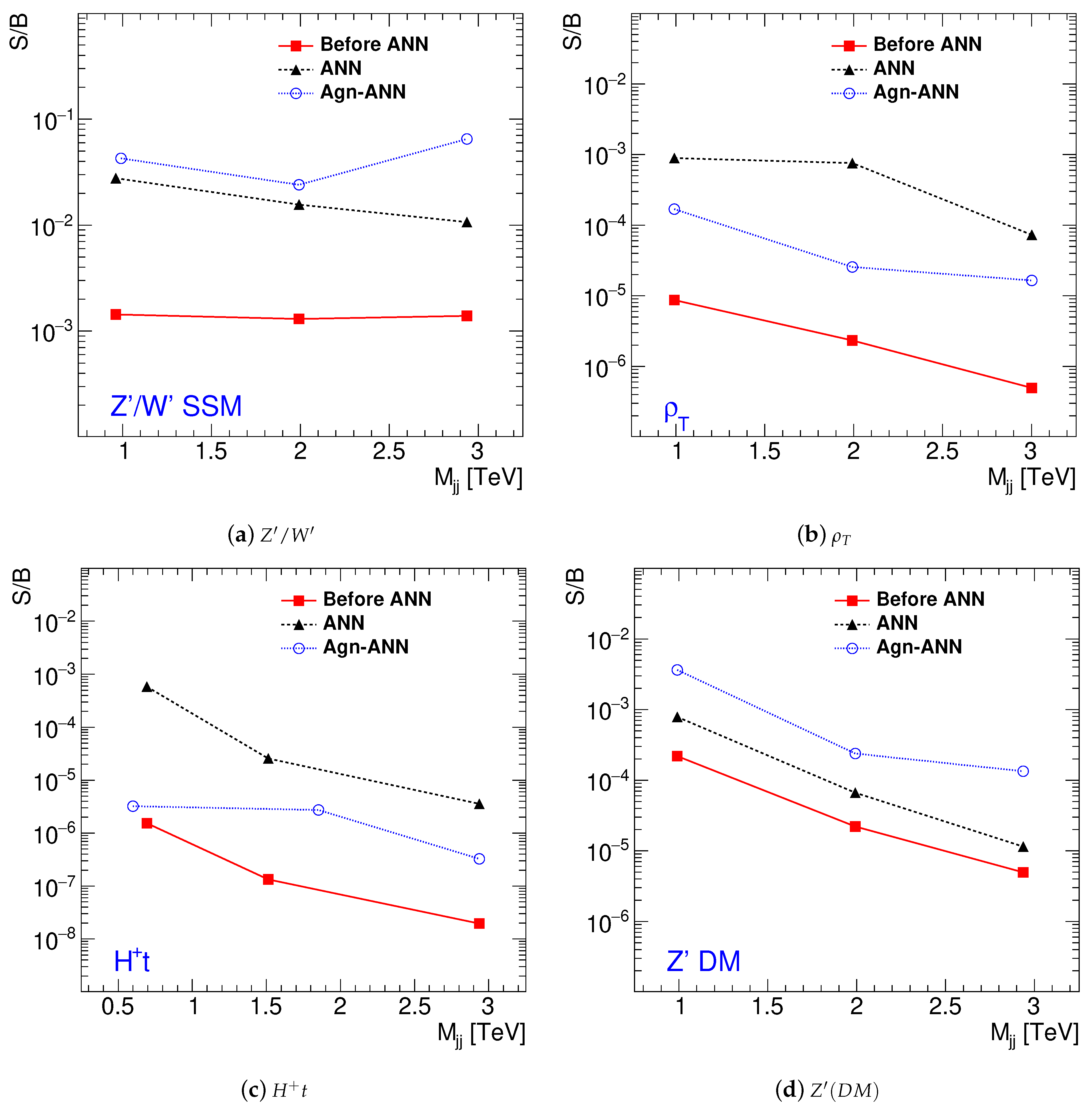
Figure 6 shows the values of the S/B ratios for the BSM models discussed in Figure 5. The ratios were defined by dividing the numbers of events of the BSM signal distributions by the number of events in the SM background near the mass regions with the largest numbers of BSM events of the distributions. The widths of the regions around the peak positions, where the events were counted, correspond to the root mean square of the histograms for the BSM models. The S/B ratios are shown for the original distribution before applying the ANN, after applying the RMM–ANN method assuming that the output ANN scores are larger than 0.2 on the output node that corresponds to the given BSM process (labeled as “ANN”) and for the model-independent RMM–ANN (“agnostic”) selection (the column “Agn-ANN”). The latter S/B ratios were obtained by removing the SM events after requiring that the output scores on the SM nodes should have values smaller than 0.8, after using RMM–ANN training without the BSM events.
This example shows that the S/B ratio can be increased by the RMM–ANN by a factor of 10–500, depending on the masses and process types. It can be seen that the S/B ratios for the and models have a larger increase for BSM-specific selection (“ANN”) compared to the BSM-agnostic selection (“Agn-ANN”). The other two BSM models show that the model-agnostic selection can even outperform the BSM-specific selection.
The latter observation is rather important. It shows that the RMM–ANN method can be used for designing model-independent searches for BSM particles without knowledge of specific BSM models. In the training procedure, the neural network “learns” the kinematic of identified particles and jets from SM events produced by Monte Carlo simulations. Then, the trained ANN can be applied to experimental data to create a sample of events that is distinct from the SM processes; i.e., that may contain potential signals from new physics. The ANN trained using the SM events, in fact, represents a numeric filter with kinematic characteristics of the SM expressed in terms of the trained neuron connections after using the RMM inputs.
A few additional comments should follow:
- The removal of the cells associated with the may not be required for model-agnostic searches since the current procedure does not use BSM models with specific masses of heavy particles. When such cells are not removed, the S/B ratio was increased by 20% compared to the case when the cell removal was applied;
- The observed increase in the S/B ratio was obtained for processes that already have significant similarities in the final states since they include leptons and jets. If no lepton selection is applied to the multi-jet QCD sample, the S/B ratio will show a larger improvement compared to that shown in Figure 6;
- For simplicity, this study combines the W+jet, Z+jets, Higgs, , and single-top events into a single event sample with a single output ANN node. The performance of the ANN is expected to be better when each distinct physics process is associated with its own output node since more neutron connections will be involved in the training;
- As a cross-check, an ANN with two hidden layers, with 300 and 150 nodes in each, was studied. Such a “deep” neural network had 3056 neurons with 826,052 connections (and 3060 neurons and 826,656 connections in the case with six outputs). The training took more time than in the case of the three-layer “shallow” ANN discussed above. After the termination of the training of the four-layer ANN using a validation sample, no improvement for the S/B ratio was observed compared to the three-layer network.
Model-independent searches using convolutional neural networks (CNN) applied to background events were discussed in [18] in the context of jet “images”. The approach based on the RMM–ANN model does not directly deal with jet shape and sub-structure variables since they are not a part of the standard RMM formalism. The goal of this paper is to illustrate that even the simplest neural networks based on the RMM feature (input) space, which reflects the kinematic features of separate particles and jets, show benefits over the traditional cut-and-count method (more detail about this can be found in Section 5). The statement about the benefit is strengthened by the fact that no detailed studies of input variables are required during the preparation step for machine learning since the RMMs can automatically be calculated for any event type. There is little doubt that more complex neural networks, such as CNNs, could show even better performance than the simplest ANN architecture used in this paper. However, comparisons of different machine learning algorithms with the RMM inputs are beyond the scope of this paper.
5. QCD Dijet Challenge
A more challenging task is to classify processes that have a mild difference between their final states. As an example of such processes, we consider the following two event types: and . Unlike the processes discussed in the previous sections, the final state consists of two jets from the hard LO process and a number of jets from the parton shower followed by hadronization. The event signatures of these two SM processes are nearly identical in terms of particle composition. Perhaps the best-known variable for separation of and dijets is the number of jet constituents. This number is larger for gluon-initiated jets due to a larger gluon color factor () compared to the quark color factor (). This can be seen in Figure 7a. Therefore, we will use the number of jet constituents of leading and sub-leading jets for ANN training. Note that jet shape and jet substructure variables can also be used (see, for example, [19]), but we limit our choice to the number of jet constituents which are outside the standard definition of the RMM.
The presence of an extra gluon in the process compared to leads to small modifications of some event characteristics. For example, Figure 7b,c shows the distributions of the number of jets per event and the transverse momentum of leading in jets. None of the analyzed kinematic distributions indicate significant differences between and so that these processes can easily be separated using cut-and-count methods.
The standard procedure for and event separation is to hand-pick variables with expected sensitivity to differences between jets initiated by quarks and gluons. Generally, a guiding principle for defining the feature space in such cases does not exist. In addition to the number of jet constituents for two leading jets, the following five input variables were selected: the total number of jets above the GeV, jet transverse momentum, rapidity and the number of constituents of two leading jets, which also show some sensitivity to the presence of the gluon shown in Figure 7b,c. Since the ANN variables need to be defined using some arbitrary criteria, we will call this approach “pick-and-use“ (PaU). Thus, the final ANN consists of seven input nodes, five hidden nodes and one output node, with zero values for the process and one for .
In the case of the RMM approach, instead of the five variables from the PaU method, we used the standard RMM discussed in the previous sections. Thus, the input had the RMM plus the number of jet constituents (scaled to the range [0, 1]). This led to 36 + 2 input nodes. The output contained one node with the value 1 for and 0 for events.
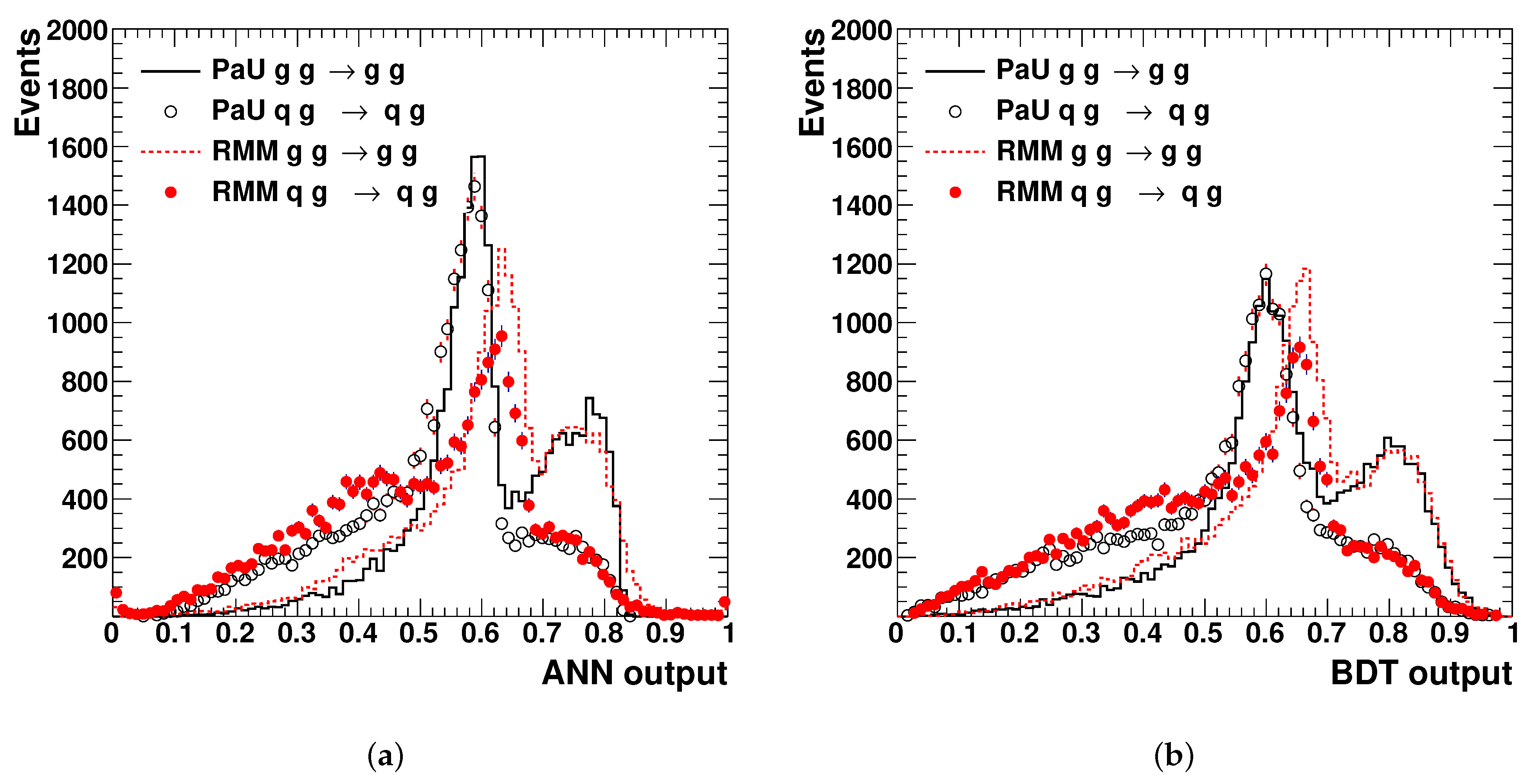
The ANN training was stopped after using a control sample. The results of the trained ANN are shown in Figure 8a. One can see that and processes can be separated using a cut at around 0.5 on the ANN output. The separation power for the PaU and RMM is similar but not the same: the separation between and for the RMM is better than for the PaU method. The PaU method leads to a purity of 65% in the identification of the process after accepting events with output node values larger than 0.5. The selection purity is 68% for the RMM inputs. The main benefit of the latter approach is the fact that the RMMs simplify the usage of machine learning, eliminating both a time-consuming feature-space study, as well as sources of ambiguity in preparing the input variables.
It is important to note that the standard RMM input can bring rather unexpected improvements for event classifications that can easily escape attention in the case of a handcrafted input for machine learning. For example, has a larger rate of isolated radiated photons of the quark from the hard process (this can be found by analyzing the RMM images). This leads to an additional separation power for the RMM inputs. In contrast, the PaU approach relies on certain expectations. In the case of the complex final states with multiple decay channels considered in the previous sections, the identification of appropriate ANN feature space becomes a complex task with the detrimental effects of ambiguity.
It should be stated that the choice of the ANN architecture with the RMM is left to the analyzer. As a check, in addition to the back-propogation neural network, we also considered a stochastic gradient-boosted decision tree with the PaU and RMM variables. The boosted decision tree (BDT) was implemented using the FastBDT package [20]. The BDT approach used 100 trees with a depth of 5. Figure 8b, confirms that the separation of from was more effective for the RMM inputs. However, the overall separation was found to be somewhat smaller for the BDT compared to the ANN method.
6. Conclusions
The experiments presented in this paper demonstrate that the RMM transformation for supervised machine learning provides an effective framework for general event classification problems. In particle physics, machine learning algorithms typically use handcrafted subject-specific variables. Such variables can be replaced by the standard RMMs, which are sensitive to a broad class of final-state phenomena in particle collisions by design. As a result, the tedious engineering of the ANN input space for different event types can be automated. At the same time, wide and shallow neural networks with multiple output nodes can be used. This paper demonstrates several such applications using the simplest back-propogration ANN and BDT techniques. It was shown that such algorithms are appropriately convergent during the training. Among several examples presented in this paper, the model-independent search that uses the ANNs trained on SM backgrounds only is an interesting direction for research into model-independent BSM searches.
Funding
The submitted manuscript has been created by UChicago Argonne, LLC, Operator of Argonne National Laboratory (“Argonne”). Argonne, a U.S. Department of Energy Office of Science laboratory, is operated under Contract No. DE-AC02-06CH11357. The U.S. Government retains for itself, and others acting on its behalf, a paid-up nonexclusive, irrevocable worldwide license in said article to reproduce, prepare derivative works, distribute copies to the public, and perform publicly and display publicly, by or on behalf of the Government. The Department of Energy will provide public access to these results of federally sponsored research in accordance with the DOE Public Access Plan. http://energy.gov/downloads/doe-public-access-plan. Argonne National Laboratory’s work was funded by the U.S. Department of Energy, Office of High Energy Physics under contract DE-AC02-06CH11357.
Institutional Review Board Statement
Not applicable.
Informed Consent Statement
Not applicable.
Data Availability Statement
The used MC data are available from the HepSim repository [8].
Acknowledgments
V. Pascuzzi, A. Milic, W. Islam and H. Meng are gratefully acknowledged for providing Monte Carlo settings for the BSM models used in this paper. V. Pascuzzi is especially acknowledged for their discussions of the machine learning methods used in this paper.
Conflicts of Interest
No conflict of interest.
Appendix A
An example of the RMM matrix with two object types, jets (j) and muons (), is shown in Equation (A1). The maximum number for each particle types in this example is fixed to a constant N. The first element at the position (1, 1) contains an event missing transverse energy scaled by , where is a center-of-mass collision energy. Other diagonal cells contain the ratio , where is the transverse energy of a leading in object i (a jet or ), and transverse energy imbalances
for a given object type i. All variables of the RMM are strictly ordered in transverse energy; i.e., . The non-diagonal upper-right values are , where are two-particle invariant masses. The first row contains transverse masses of objects for two-body decays with undetected particles, scaled by , i.e., . The first column vector is , where y is the rapidity of a particle , and C is a constant defined such that the average values of are similar to those of and , which is important for certain algorithms that require input values to have similar weights. The value is constructed from the rapidity differences between i and j.
References
- Chekanov, S.V. Imaging particle collision data for event classification using machine learning. Nucl. Instrum. Meth. 2019, 931, 92–99. [Google Scholar] [CrossRef] [Green Version]
- Santos, R.; Nguyen, M.; Webster, J.; Ryu, S.; Adelman, J.; Chekanov, S.; Zhou, J. Machine learning techniques in searches for h in the h→ decay channel. J. Instrum. 2017, 12, P04014. [Google Scholar] [CrossRef] [Green Version]
- Sjostrand, T.; Mrenna, S.; Skands, P.Z. PYTHIA 6.4 Physics and Manual. J. High Energy Phys. 2006, 5, 026. [Google Scholar] [CrossRef]
- Sjostrand, T.; Mrenna, S.; Skands, P.Z. A Brief Introduction to PYTHIA 8.1. Comput. Phys. Commun. 2008, 178, 852–867. [Google Scholar] [CrossRef] [Green Version]
- Ball, R.D.; Bertone, V.; Carrazza, S. Parton distributions for the LHC Run II. J. High Energy Phys. 2015, 4, 040. [Google Scholar] [CrossRef] [Green Version]
- Buckley, A.; Ferrando, J.; Lloyd, S.; Nordström, K. LHAPDF6: Parton density access in the LHC precision era. Eur. Phys. J. 2015, 75, 132. [Google Scholar] [CrossRef] [Green Version]
- Akeroyd, A.G. Prospects for charged Higgs searches at the LHC. Eur. Phys. J. 2017, C 77, 276. [Google Scholar] [CrossRef]
- Chekanov, S.V. HepSim: A repository with predictions for high-energy physics experiments. Adv. High Energy Phys. 2015, 2015, 136093. Available online: http://atlaswww.hep.anl.gov/hepsim/ (accessed on 1 February 2019). [CrossRef] [Green Version]
- Cacciari, M.; Salam, G.P.; Soyez, G. The anti-kt jet clustering algorithm. J. High Energy Phys. 2008, 4, 063. [Google Scholar] [CrossRef] [Green Version]
- Cacciari, M.; Salam, G.P.; Soyez, G. FastJet User Manual. Eur. Phys. J. 2012, 72, 1896. Available online: http://fastjet.fr/ (accessed on 1 February 2019). [CrossRef] [Green Version]
- Aad, G. (ATLAS Collaboration) Performance of b-Jet Identification in the ATLAS Experiment. J. Instrum. 2016, 11, P04008. [Google Scholar] [CrossRef]
- Aad, G. (ATLAS Collaboration) Expected Performance of the ATLAS Experiment—Detector, Trigger and Physics. Preprint CERN-OPEN-2008-020. 2009. Available online: http://cds.cern.ch/record/1125884 (accessed on 18 January 2021).
- Nissen, S. FANN. Fast Artificial Neural Network Library. Web Page. Available online: http://leenissen.dk/fann/wp/ (accessed on 1 February 2019).
- Altarelli, G.; Mele, B.; Ruiz-Altaba, M. Searching for new heavy vector bosons in colliders. Z. Phys. C 1989, 45, 109. [Google Scholar] [CrossRef]
- Eichten, E.; Lane, K.D.; Womersley, J. Finding low scale technicolor at hadron colliders. Phys. Lett. 1997, 405, 305–311. [Google Scholar] [CrossRef] [Green Version]
- Abercrombie, D. Dark Matter Benchmark Models for Early LHC Run-2 Searches: Report of the ATLAS/CMS Dark Matter Forum. arXiv 2015, arXiv:1507.00966. [Google Scholar] [CrossRef]
- Aad, G. Search for Dijet Resonances in Events with an Isolated Lepton Using = 13 TeV Proton–Proton Collision Data Collected by the ATLAS Detector; Technical Report ATLAS-CONF-2018-015; CERN: Geneva, Switzerland, 2018. [Google Scholar]
- Farina, M.; Nakai, Y.; Shih, D. Searching for New Physics with Deep Autoencoders. arXiv 2018, arXiv:1808.08992. [Google Scholar] [CrossRef] [Green Version]
- Gallicchio, J.; Schwartz, M.D. Quark and Gluon Tagging at the LHC. Phys. Rev. Lett. 2011, 107, 172001. [Google Scholar] [CrossRef] [PubMed] [Green Version]
- Keck, T. FastBDT: A speed-optimized and cache-friendly implementation of stochastic gradient-boosted decision trees for multivariate classification. arXiv 2016, arXiv:1609.06119. [Google Scholar]
- Map2RMM Library. Available online: https://atlaswww.hep.anl.gov/asc/map2rmm/ (accessed on 18 January 2021).
| 1. | The RMM + ANN training with 100 epochs took 3 h using 16 threads of the Intel Xeon E5-2650 (2.20 GHz) CPU. |
Figure 1.
Visualization of the rapidity–mass matrixes (RMMs) for (a) multijet QCD events and (b) for the Standard Model Higgs production (all decays of the Higgs are allowed). The definition of the RMM is given in the text. The RMMs were obtained after averaging over 100,000 collision events generated using Pythia8 after parton showers and hadronization. The several empty cells shown in white color are due to the lack of statistics.

Figure 2.
Variation of mean squared error (MSE) vs. the number of epochs for the training and validation RMM data. The MSE for training and validation samples are similar for a small number of epochs. The large oscillations in MSE are due to finding the most optimal weights in the presence of empty RMM cells (which are similar for the validation and training sample). The deviation between the training and validation sample after 100 epochs indicates over-training.

Figure 3.
The ANN output scores for Monte Carlo events with the charged Higgs (), Standard Model (SM) Higgs, ,
and double production. The black solid lines show the output for a given (known) event category. Other lines show
the values of other nodes in the output ANN layer. The collision events were generated using Pythia8 after parton
showers and hadronization. All decays of heavy bosons and top quarks allowed by the Pythia8 were included.


Figure 4.
The artificial neural network (ANN) output scores for the output nodes of the beyond Standard Model (BSM) models for the background (thick black and blue solid lines) and those corresponding to the BSM model for different mass assumptions (red lines). The collision events were generated using Pythia8 after parton showers and hadronization.

Figure 5.
The distributions for 150 fb of collisions at TeV for the background and BSM models (shown for three representative masses of heavy particles) before and after applying the RMM–ANN selections. (b,e,h,k) use a cut on the ANN scores for the BSM output nodes. (c,f,i,l) show a model-independent selection that does not use BSM events for the ANN training.

Figure 6.
The values of the signal-over-background (S/B) ratios for three masses of BSM heavy particles that create peaks. The values are shown for the original distribution, after applying cuts on the output nodes of the corresponding BSM event types (labeled as “ANN”), and for a model-independent (agnostic) selection (labeled as “Agn-ANN”) without using the BSM events for the ANN training. The latter S/B ratios were obtained by filtering out the SM processes after requiring that the SM output nodes should have values smaller than 0.8.

Figure 7.
The comparison between several distributions for and processes. The collision events were generated using Pythia8 after parton showers followed by hadronization. (a) The distributions of the number of jet constituents (for all jets above GeV). (b) The distribution of the numbers of jets. (c) The transverse momentum of jets leading in .

Figure 8.
(a) The ANN output for and events in the case of a “pick-and-use“ (PaU) approach based on seven selected input variables and the RMM. (b) The output of the boosted decision tree (BDT) for the same inputs as in (a). The events were generated using Pythia8 after parton showers followed by hadronization.

Publisher’s Note: MDPI stays neutral with regard to jurisdictional claims in published maps and institutional affiliations. |
© 2021 by the author. Licensee MDPI, Basel, Switzerland. This article is an open access article distributed under the terms and conditions of the Creative Commons Attribution (CC BY) license (http://creativecommons.org/licenses/by/4.0/).
Share and Cite
MDPI and ACS Style
Chekanov, S.V. Machine Learning Using Rapidity-Mass Matrices for Event Classification Problems in HEP. Universe 2021, 7, 19. https://doi.org/10.3390/universe7010019
AMA Style
Chekanov SV. Machine Learning Using Rapidity-Mass Matrices for Event Classification Problems in HEP. Universe. 2021; 7(1):19. https://doi.org/10.3390/universe7010019
Chicago/Turabian StyleChekanov, Sergei V. 2021. "Machine Learning Using Rapidity-Mass Matrices for Event Classification Problems in HEP" Universe 7, no. 1: 19. https://doi.org/10.3390/universe7010019
Note that from the first issue of 2016, this journal uses article numbers instead of page numbers. See further details here.