Model Predictive Control for the Process of MEA Absorption of CO2 Based on the Data Identification Model


1
College of Electrical and Information Engineering, Lanzhou University of Technology, Lanzhou 730050, China
2
Key Laboratory of Gansu Advanced Control for Industrial Processes, Lanzhou 730050, China
3
College of Physics and Electrical Engineering, Weinan Normal University, Weinan 714000, China
*
Author to whom correspondence should be addressed.
Processes 2021, 9(1), 183; https://doi.org/10.3390/pr9010183
Submission received: 21 December 2020
/
Revised: 8 January 2021
/
Accepted: 14 January 2021
/
Published: 19 January 2021
(This article belongs to the Special Issue Carbon Capture and Utilisation)
Abstract
:The absorption process of CO by ethanolamine solution is essentially a dynamic system, which is greatly affected by the power plant startup and flue gas load changes. Hence, studying the optimal control of the CO chemical capture process has always been an important part in academic fields. Model predictive control (MPC) is a very effective control strategy used for such process, but the most intractable problem is the lack of accurate and effective model. In this work, Aspen Plus and Aspen Plus Dynamics are used to establish the process of monoethanolamine (MEA) absorption of CO related models based on subspace identification. The nonlinear distribution of the system under steady-state operation is analyzed. Dynamic tests were carried out to understand the dynamic characteristics of the system under variable operating conditions. Systematic subspace identification on open-loop experimental data was performed. We designed a model predictive controller based on the identified model combined with the state-space equation using Matlab/Simulink to analyze the changes of the system under two different disturbances. The simulation results show that the control performance of the MPC algorithm is significantly better than that of the traditional proportion integral differential (PID) system, with excellent setpoint tracking ability and robustness, which improve the stability and flexibility of the system.
1. Introduction
Since the industrial revolution, the increase of CO content in the atmosphere has led to the increase of the greenhouse effect year by year, which leads to a series of extreme weather problems [1,2,3]. CO emissions come mainly from the combustion of fossil fuels, especially coal-fired power plants, which are recognized as point sources of CO emissions that exacerbate greenhouse effects. The capture and recovery of CO are the key measures for effective emission reduction [4]. Compared with other carbon dioxide capture theories, the post-combustion amine capture technology is the closest technology to commercial operation and is suitable for the transformation of existing power plants. It is the mainstream technology of carbon capture at present [5,6,7].
Hence, since the implementation of the Post-combustion CO Capture Process (PCCP), scholars in the process control field and engineers have invested a lot of time and money to solve and improve the capture performance of CO capture systems [8]. U.S. technology company CANSOLV achieved cost reduction by combining CO capture and capture of pollutants, such as CO, nitrogen oxides, and mercury [9]. The Center for International Cooperation on CO Capture, Storage and Utilization (iCCSU), established by Professor Tong Baidong, Hunan University in September 2009, has carried out fruitful applied basic research and key technology development on the frontier of CO capture, separation and purification, and solidification of carbon dioxide materials [10].
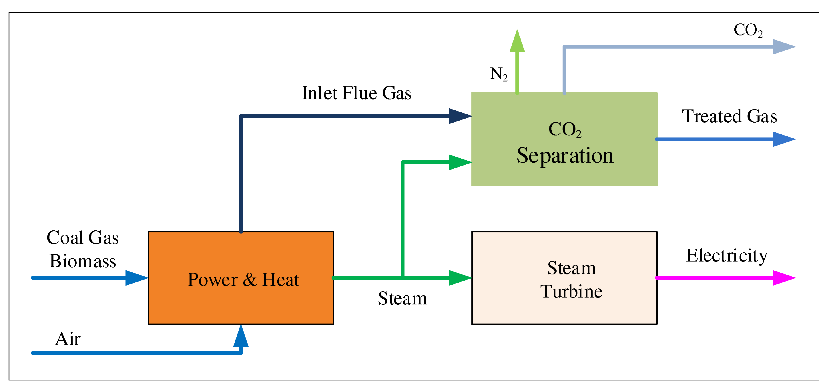
Regarding the industrial process, under the background of the chemical process industry, the improvement space of the process operation will always exist. In view of the technology that PCCP can improve the efficiency of power generation by improving the operation process, scholars have carried out a lot of research in recent years [11,12]. Figure 1 shows traditional power plants and carbon dioxide capture processes.
Shan et al. [13] proposed a model of absorption tower and desorption tower based on the kinetic relationship between the column enhancement factor and the chemical reaction and verified it in MATLAB/Simulink. In [14], under the open loop condition, the flue gas flow is fixed, and the other inputs remain constant. The dynamic response of the absorption tower model established in Modelica is compared with the dynamic response in the actual plant, and the correctness of the absorption tower model is verified. In terms of model establishment, the above studies only verified a certain link of the system, and did not conduct a systematic dynamic analysis of the overall model. On this basis, Lin et al. [15] established a complete CO capture system model in Aspen Plus Dynamics and determined the factors that affect CO removal performance, energy efficiency, and the long-term stability of the absorption/stripping CO capture process using monoethanolamine solution. Three important factors, namely lean solvent flow rate, lean solvent load, and water replenishment of the balance system, provide guidance for the dynamic modeling of the CO capture system. Kvamsdal et al. [16] designed a CO dynamic capture model based on the rate level in Matlab and compared the data obtained in the steady-state and dynamic tests with the data collected in VOCC (validation of carbon capture) to verify the accuracy of the model when the absorption tower is in a specific working condition. Subraveti et al. [17] established an equilibrium model based on the post-combustion CO capture model in Modelica and used steady-state experimental data to adjust the model coefficients related to mass/heat transfer and chemical reactions to make the model more suitable for actual plants under nominal operating conditions.
The study of PCCP operation control by Mechleri et al. [18] was carried out using conventional single-loop disturbance suppression methods, such as stabilizing the CO content of the intake channel, keeping the steam temperature and heat capacity of the reboiler constant, maintaining the MEA content of the stripping unit constant, etc. Lin et al. proposed two different proportional-integral (PI) control strategies to maintain the desired absorption efficiency by using the lean solvent flow rate and reboiler input heat as manipulation variables [19]. Beedelbayev et al. gave the single machine type only for the absorber MPC control scheme [20]. Panahi and Skogtogad implemented a MPC control strategy using the degree of CO recovery and reboiler temperature as controlled variables [21,22]. From the current research situation, existing PCCP dynamic research focuses on the study of the dynamic characteristics of a single tower or a single unit and simple PI control algorithms.
However, the complete dynamic performance of the capture rate of the actual power plant PCCP device under the condition of flue gas disturbance is still lacking. In variable operating conditions, the control effect is not particularly ideal. For the purpose of solving the problem of the slow response and system constraint of PCCP regulating systems in variable working conditions, Section 1 introduces the background, motivation, and contribution. Section 2 introduces the dynamic behavior of the system, establishes the complete CO capture system in the Aspen Plus and Aspen Plus Dynamics, and determines the state space model with high fitting degree according to the experimental data in Section 3. Section 4 shows the design of the MPC controller in the Matlab/Simulink and establishes the capture rate adjustment model of the CO capture system; the system simulation is qualitatively analyzed according to the performance index. It is found that the MPC algorithm can achieve the given capture rate results more accurately and stably than the conventional PID algorithm regulation system, and the regulation system has good control performance, which provides a reference for the flexible design of the PCCP capture rate.
2. Description of the Post-Combustion Capture CO System
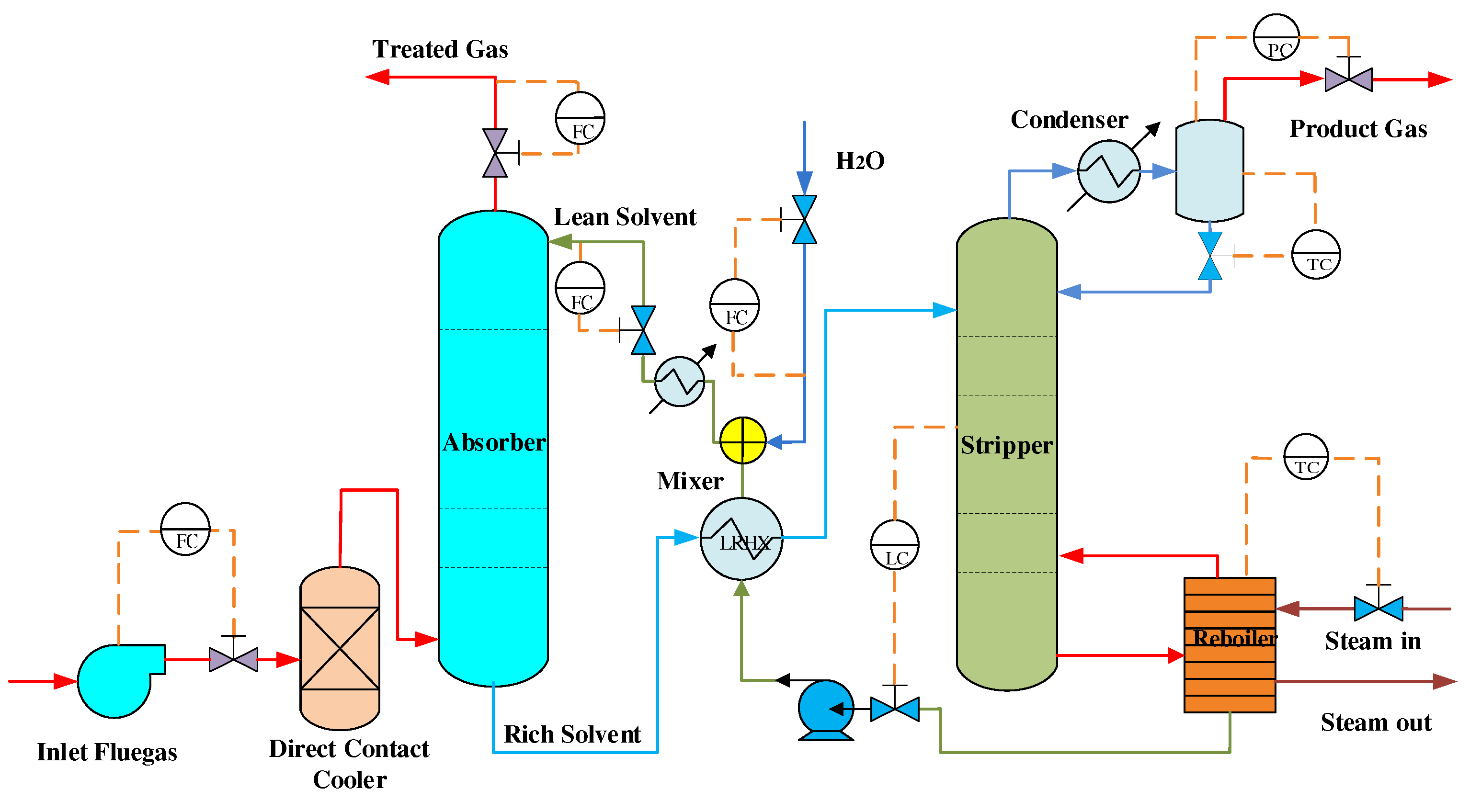
Studies have shown that the core of CO capture technology is to improve the operation process by implementing advanced control technology on the CO capture device. MEA is the best choice for the CO absorbent with its absorptivity of up to 90% [23,24]. Therefore, capture CO equipment and its process based on MEA combustion are the most commercially attractive options in the world. Figure 2 shows a schematic diagram of the CO capture device after combustion in an amine-based power plant.
As shown in Figure 2, after desulfurization [25], the flue gas reacts with the MEA solvent flowing into the top of the tower by fan pressurization to remove carbon dioxide from the furnace gas. The rich liquid absorbs carbon dioxide from the bottom of the absorption unit and then heats up into the stripping unit. The lean solvent produced by the reaction is recycled from the bottom of the stripping unit to the absorption unit, and the analytical carbon dioxide is purified. Finally, the high-pressure carbon dioxide gas is used. To maintain the water balance of the system, water is replenished in the system [26].
2.1. Mathematical Model of a Post-Combustion Capture CO System
In the mathematical model, the description of the absorption unit and the stripping unit is consistent. The difference is that the reboiler unit is added to the stripping unit and the gas is stripped at the high temperature produced by it. The mathematical model of each unit reflects the dynamic behavior of each part of the system.
2.1.1. Modeling Assumptions
The assumptions used in the modeling of the PCCP plant are:
- All reactions reach equilibrium.
- The velocity of any section of the axial surface is constant, and the pressure drop is linear along the axial direction of the tower.
- Mass and heat transfer are described by the two-film theory [27].
- The interface between the liquid film and the gas film is in phase equilibrium.
- Solution degradation is negligible.
- No heat losses to the surrounding area.
2.1.2. Absorption and Stripping Units
Equations (1)–(4) describe the mass and energy balances along the axial direction in the two reaction towers.
Here, (mol/m) and (mol/m) are the gas and liquid concentrations of each component, F (m/s) is phase volumetric flow, (m) is the radius of the reaction column, (mol/m/s) is the molar flux i the component, T (K) is the temperature of the liquid and gas phases, (m/ m) is the gas–liquid contact area, is the length of the reaction column, (kJ/kmol) is heat capacity, and Q (kJ/ms) is the heat transfer rate. The i components in the column are MEA, N, CO, and HO. In the absorption unit, is the operating variable to control the carbon dioxide capture rate and is a disturbance from the power plant.
2.1.3. Heat Exchanger Model
The lean-rich heat exchanger considered in the process is assumed to be a counter-current shell and tube heat exchanger.
where T (K) is the temperature, (m/s) is volume flow, V (m) is volume, (kJ/s) is the heat transfer rate, (kmol/m) represents the average molar density, and the subscripts tube, shell, in, and out represent the management side, shell side, inlet, and outlet of the heat exchanger, respectively.
2.1.4. Reboiler Model
In the reboiler unit, the CO-absorbed rich solvent is heated to break the chemical bond between the CO and MEA. The remaining components (HO, CO and MEA) evaporate and enter the bottom of the stripper. The solvent with low amount of CO exists from the bottom of the reboiler and enters a new cycle. Its mass and energy balance are shown in Equations (7) and (8):
The components i are MEA, CO, and HO. (kmol) is the mass holdup of component i, F (kmol/s) is the molar flow rate, F and L are the flow rates of steam and liquid, and the subscripts in and out represent the input and output. In the description of energy balance, (K) is temperature, (kmol/m) is density, (kJ/kmol) is molar heat capacity, V (m) is retention volume, H (kJ) is enthalpy, and (kJ/s) is heat input.
2.2. Steady-State and Dynamic Model
The steady-state model uses ELECNRTL physical method and CO–MEA–HO systems containing the following five equilibrium reactions to describe the absorption equilibrium in the system.
The kinetic reversible reactions involve can be expressed as:
The power plant lean solvent flowrate is 0.458 kg/s [28] and the CO capture rate is fixed at 70%. The reboiler type in the stripper is selected. Flue gas condition in PCC plant is shown in Table 1. The parameters corresponding to the absorber and the stripper are shown in Table 2.
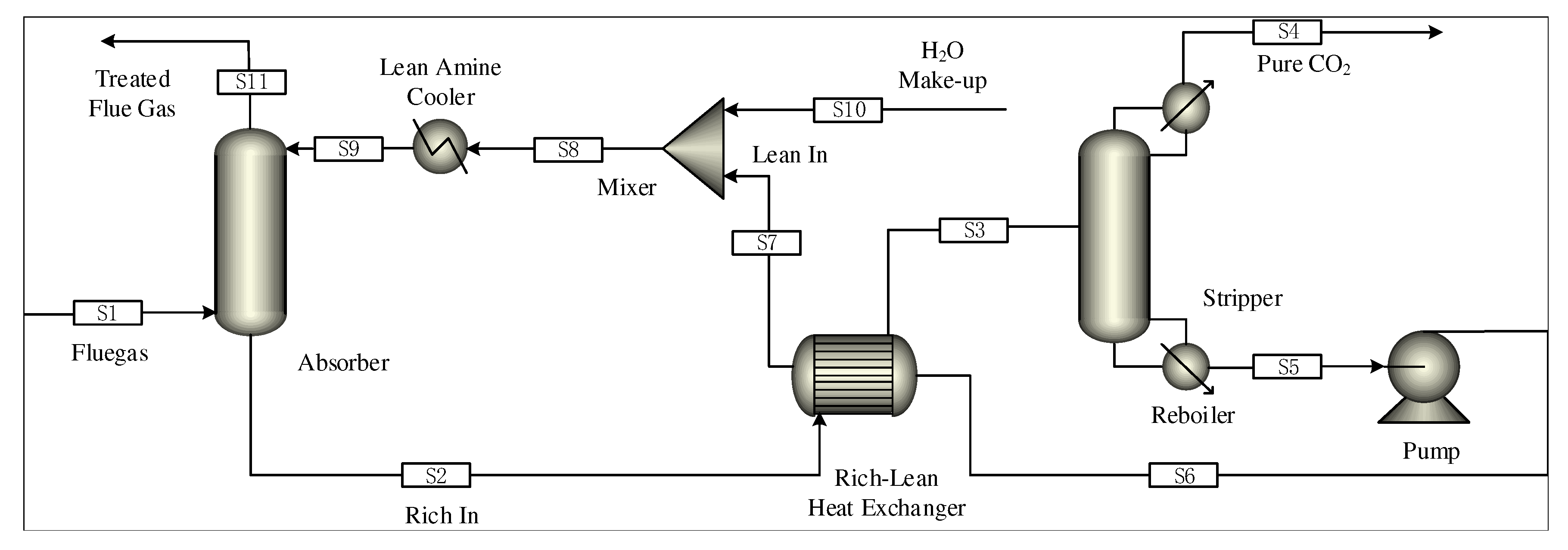
The size of absorber/stripper is added to the steady-state model under the above optimal working conditions, and the parameters needed for the dynamic models such as the liquid level and pressure are set. The steady-state model is derived as the initial value file of dynamic model driven by pressure. Compared with the equilibrium-based model, the rate-based model can predict and simulate the results more accurately. Therefore, the rate model is recognized as the most reliable process model of absorption and desorption. However, the dynamic simulation in the Aspen Plus Dynamics does not support the rate level model, so the equilibrium level model is selected in this paper [17]. The steady-state model of the post-combustion CO capture system in Aspen Plus is shown in Figure 3.
The system capture rate is defined as
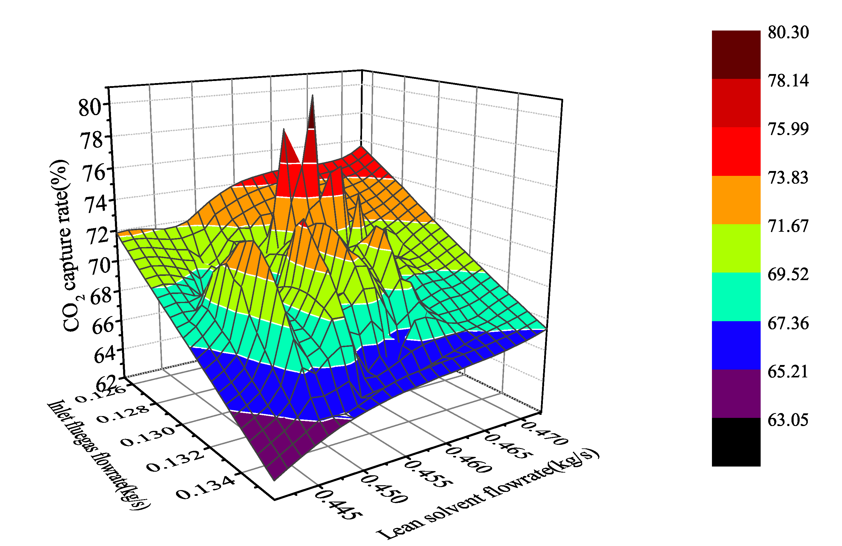
where CO% represents the CO capture rate, is the CO moles flow in flue gas, and the subscripts in and out represent exports and imports. Under the above definition, we can obtain the nonlinear distribution of carbon dioxide capture system under specified working conditions (capture rate 63.05–80.25%, flue gas flowrate 0.125–0.136 kg/s, and lean solvent flowrate 0.439–0.472 kg/s) by dynamic analysis in aspen plus dynamics (Figure 4).
According to the analysis of the trapping rate distribution in the figure, when the flue gas flow is at a high flow rate and the lean liquid flow is at a low flow rate, the capture rate is low. When the flue gas flow is at a low flow rate but the lean solvent flow is high, the system capture rate is increased quickly, which improves the ability of the collection system to operate flexibly. However, in steady state operation, only points can be taken individually to obtain singular information of a certain working condition, and it is impossible to flexibly study the changes of the system with input. Therefore, dynamic testing of the system in Aspen plus Dynamics was performed to understand that the system is dynamically changing.
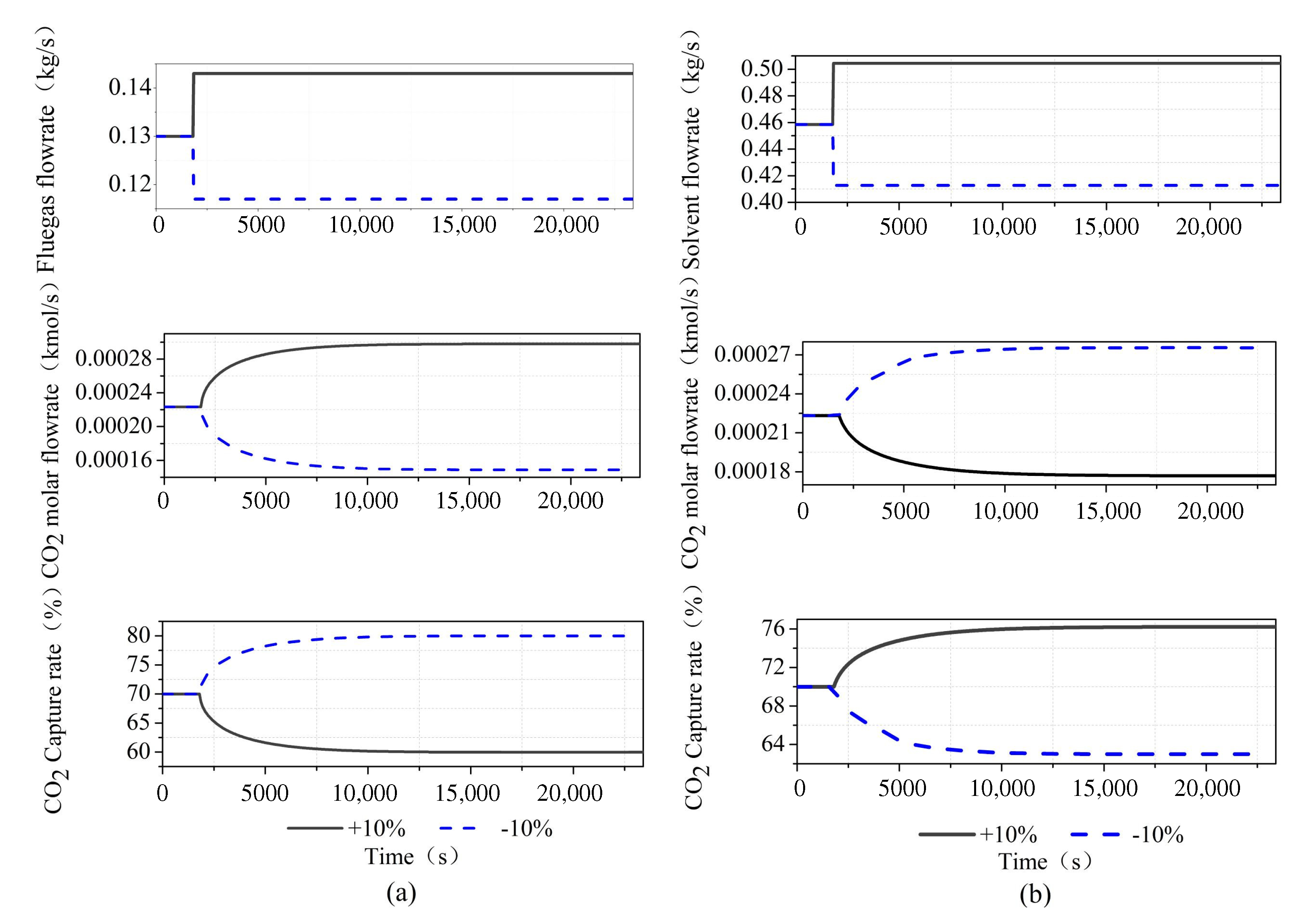
We have conducted a dynamic test on the system, as shown in Figure 5. We perturb the flue gas flow and lean solvent flow by , and it can be seen that it is consistent with the steady-state operation trend. When the flue gas flow rate increases, the MEA solution cannot completely absorb the CO in the flue gas, resulting in an increase in the outlet CO concentration and a decrease in the capture rate. When the lean solvent flow rate increases, the CO in the flue gas is completely absorbed by the MEA solution, and the carbon capture rate increases. From the viewpoint of mass transfer kinetics, according to the two-film theory analysis, the transfer of gas and liquid phases in the two-film and the absorption of CO by MEA require a certain amount of time for diffusion and material conversion. The increase in the gas flow rate reduces the reaction time of the gas–liquid phase in the film, and MEA is too late to absorb CO. Therefore, increasing the flue gas flow rate will gradually reduce the capture rate. Increasing the flow rate of the absorbent enables the limited carbon dioxide in the flue gas to be fully captured, thus greatly improving the capture rate of the system.
3. Model Predictive Control for the Post-Combustion Capture CO System
The model predictive control algorithm is the earliest computer optimization control algorithm in the industrial fields in the United States and France, developed in the late 1970s [29]. The model predictive control is based on the predictive model, rolling optimization, and feedback correction control strategy in the implementation process. These methods not only have strong robustness and better control effect but also require low accuracy of the control system model. Based on the advantages of model predictive control, it has been widely used in process control, mechanical engineering, and chemical production [30].
3.1. Model Identification
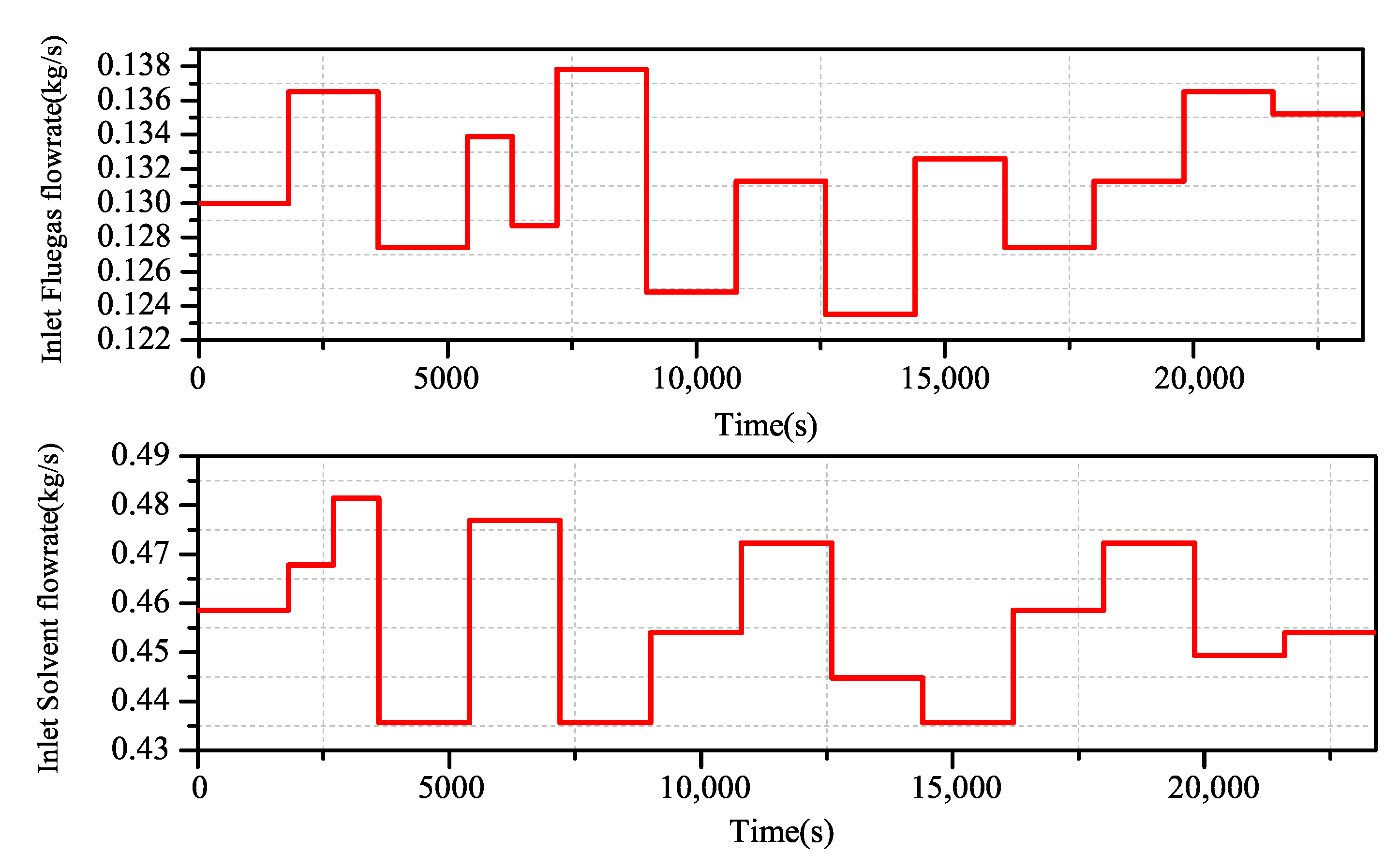
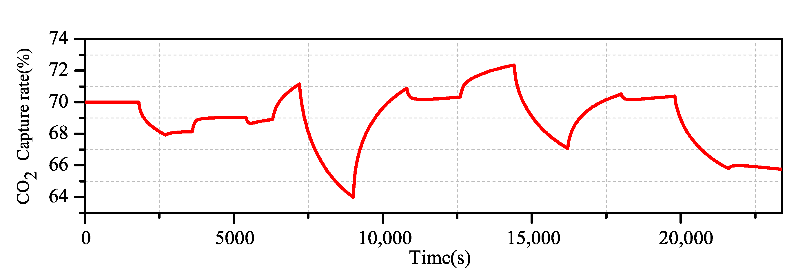
By using the Aspen Plus Dynamics software, the open loop experimental data of the change of flue gas flow and lean liquid flow on the carbon dioxide capture rate are obtained, and the excitation signal shown in Figure 6 is added to the flue gas flow end and the lean solvent flow end. The actual output of the system is obtained (Figure 7).
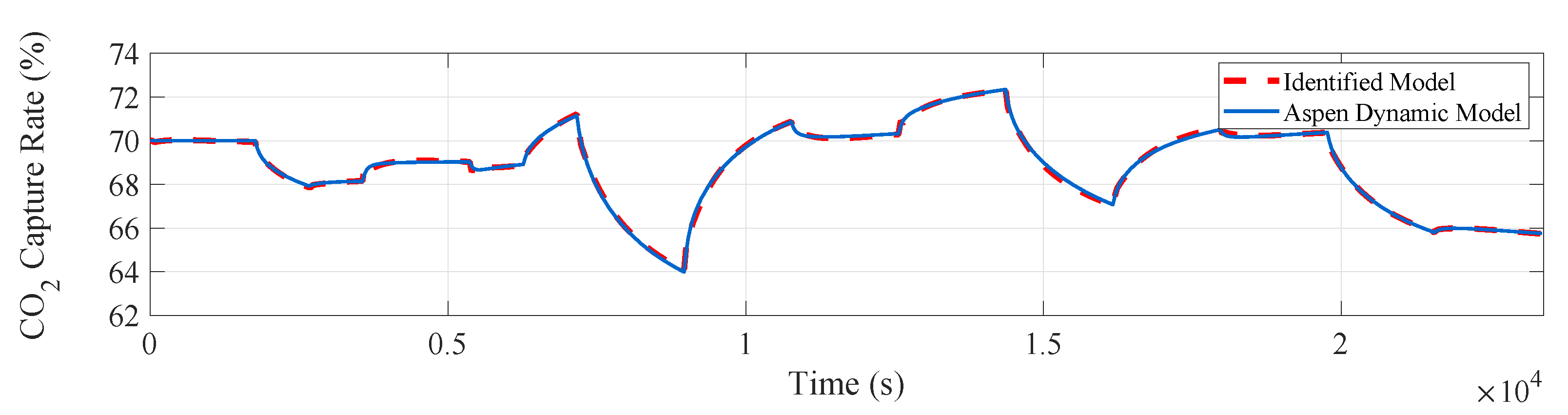
The input and output data are imported into the identification toolbox by using the system identification toolbox in Matlab. We adopt the method of subspace identification, the sampling time is 0.01 h (36 s), for subspace identification of the experimental data. The fitting curve of the actual output and model output of the system is obtained, reaching a 96.42% fitting degree and achieving a satisfactory fitting degree, which in shown in Figure 8.
The identification models of the flue gas flow rate, carbon dioxide capture rate, lean solvent flowrate, and carbon dioxide capture rate are obtained, as shown in Table 3.
By doing the open-loop disturbance experiment, we no longer need to establish the complex mechanism model of the controlled object, which is more convenient to study the control strategy.
3.2. Model Predictive Control Algorithm for the Post-Combustion Capture CO2 System
The traditional control method is usually used to solve a feedback control law offline, and the feedback control law is always applied to the system. Relative to other controls, the main feature of MPC is to solve open-loop optimization problems online and obtain open-loop optimization sequences. Its operating mechanism is mainly divided into three steps: (1) the future dynamics of the system is predicted; (2) the optimization problem is solved; and (3) the first element of the solution acts on the system.
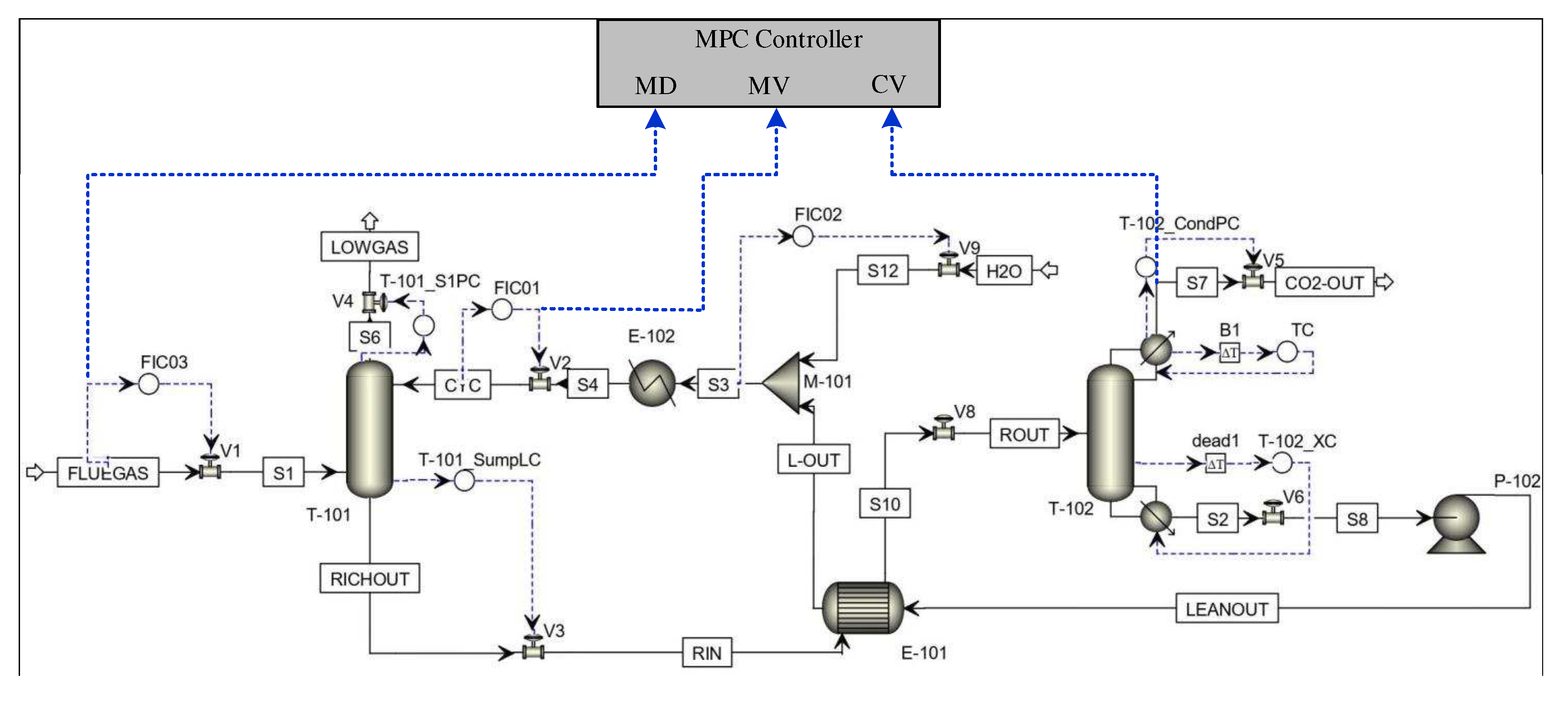
A MPC controller is designed based on model predictive control principle. Figure 9 shows the MPC control diagram of the PCCP system.
Consider the equation of state space for linear discrete-time systems
In Equation (12), is a state variable, is the control input variable, is the controlled output variable, and is a measurable external interference variable. Among them, , , and . is the lean solvent flow rate and is inlet flue gas flow rate, which is the main measurable disturbance. is the CO capture rate. A, , , and can be obtained by system identification.
First, based on the Equation (12), the future dynamics of the system is predicted with the latest measurement value as the initial condition. Prediction time domain is set as , control time domain as , and . Then, the prediction output of the future steps of the post-combustion CO capture system can be expressed by the following prediction equations:
The CO capture system objective function can be described as follows:
where is the set point for the controlled variables and and are the weighted matrices of the predicted output vector and the input vector, respectively. The goal of the optimization function is to make the capture rate of the CO capture system track the given desired trajectory as soon as possible. The first part of Equation (14) reflects the tracking ability of the system to the desired trajectory. The second part reflects the stability requirements of the control quantity. For the purpose of solving the optimization problem, the derivative of in Equation (14) can be expressed as
If Equation (15) takes zero, the solution of the minimum value is obtained from the extreme value condition, that is, the optimal control sequence at k time:
The control movement has maximum and minimum bounds of ±0.1%/s of the nominal values to prevent highly aggressive control actions.
Because, in the actual process, there is a certain constraint problem, the capture rate output is required to have no overshoot; that is, there is a constraint output
4. Simulation and Results Analysis
The dynamic characteristic model of rear combustion CO capture in a power plant with lean solvent flow as the controlled input, carbon dioxide capture rate as the controlled output, and flue gas flow as the disturbance variable as established in Matlab/Simulik. This paper takes the principles of small overshoot, fast response speed, and good tracking of a set value. The control effect of the system after combustion was verified by simulation experiments and compared with traditional PID. The key parameters of the tuning controller are shown in Table 4.
This paper generally does not adopt the differential term in the PID controller because of the more interference in the actual control in the PID control strategy. Since the sampling time is 0.01 h in the actual chemical simulation and system identification, the sampling time in this paper is 36 s. First, both kinds of simulation add Gaussian distributed random signal.
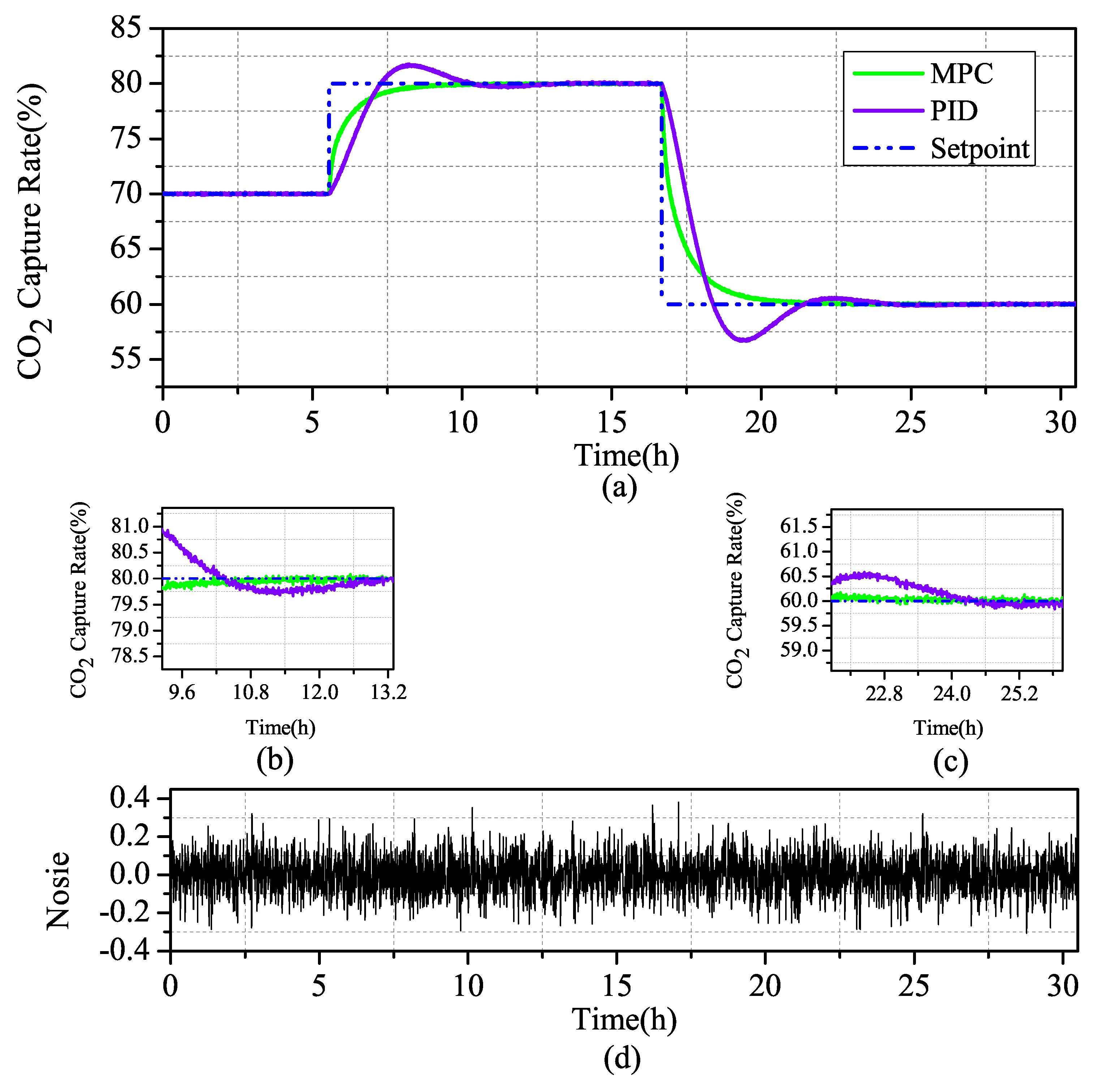
Transient response to a step change of lean solvent flow: In Scenario 1 of a given reference value input to a two-segment step signal, when the system runs stably for 4.1 h, the system steps up under the condition of a setting value of 70% and changes the setting value to 80%. When the system is under stable operation, at 18.0 h, the set value is reduced from 80% to 60%, and the stability of the controller design is investigated.
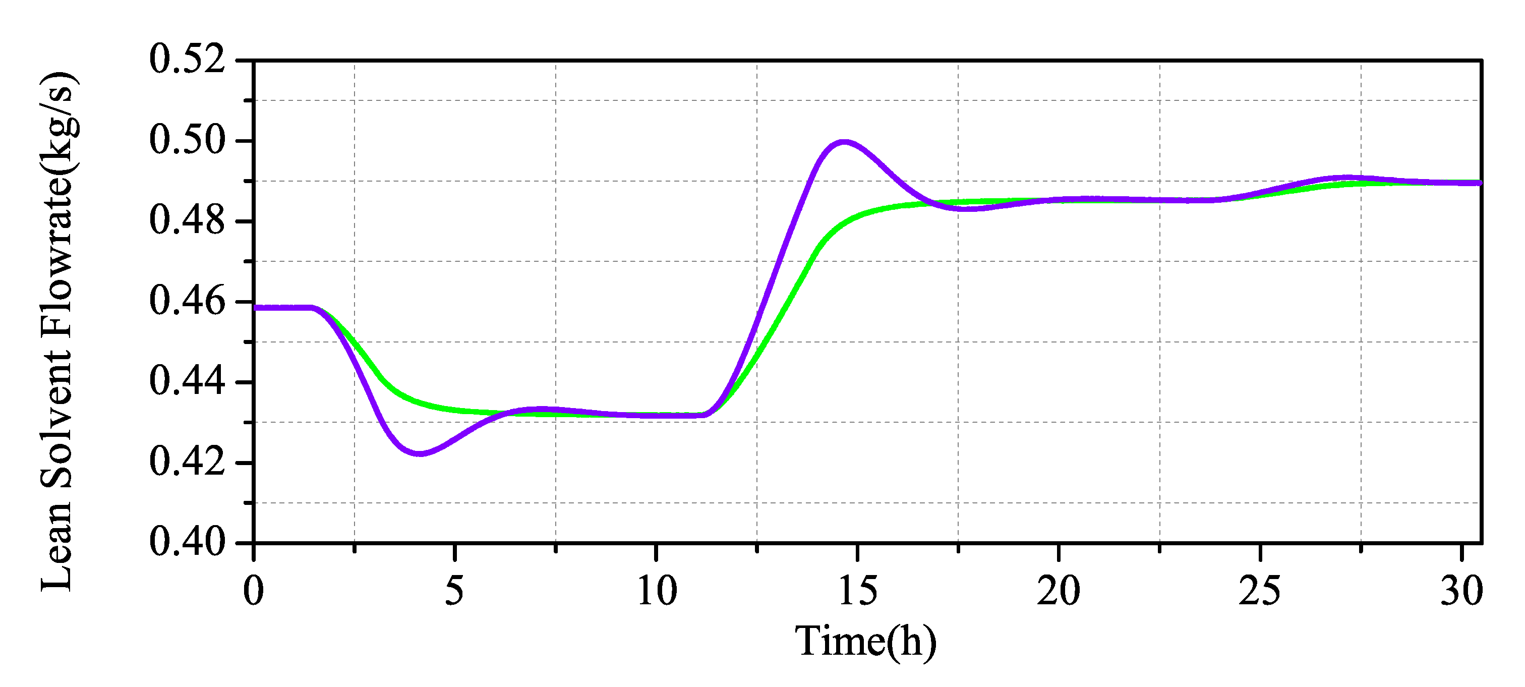
Transient response to a ramp change of lean solvent flow: Scenario 2 starts with steady-state operation. The three-stage slope signal was investigated: (a) at 1.4 h, to give reference to the descent ramp signal and decreased to 15% at a rate of 9%/h; (b) at this stage of steady operation to 11.1 h, a rising signal at a rate of 10.8%/h, steady state operation to 23.6 h; and(c) at 23.6 h, at a rate of 0.9%/h, and stable operation to 3.0 h, comprehensively consider the stability of the MPC and PID control when the system is undergoing a large decline, a large rise, and a small rise.
The simulation results in Figure 10 and Figure 11 show that the output of the CO capture system increases with the increase of the measured input value, which is in line with the actual process. When the system changes slightly, the overshoot of the PID is not high, but the MPC has almost no overshoot. When the system decreases greatly, the overshoot of the PID increases obviously, while the overshoot of the MPC maintains almost no overshoot stability.
The results in Table 5 show that, in terms of rapid performance, the CO capture system under MPC control is higher than that under traditional PID control, although the rise time are higher than those under PID control. Under the MPC control strategy and the PID control strategy, the overshoot difference is two orders of magnitude, which is obviously better than the control. When the steady-state time of the system is analyzed, it can be seen that, under the condition of sudden change of set value, the system under MPC control can pull the system back to the stable state more quickly, while the traditional PID still has to go through a large fluctuation before it can gradually stabilize. The robustness of MPC is greatly improved compared with that of PID, by multiplying the absolute value error integral by time. According to the overall analysis, the MPC achieved a better control effect.
Through the comparative analysis of Figure 12 and Figure 13, it can be seen that MPC and PID control strategies can control the system in a stable state after a period of time, but, in terms of stability, MPC is obviously better than PID, for control effect. During the large change of the system, the fluctuation of the PID adjusted system changes greatly, and only after two periods of fluctuation near the set value can the set value be returned. During the small change of the system, although the PID has a small shock, it quickly returns to the set value. It can be seen that the regulation performance is still better in PID when faced with small changes in the system, but, in MPC, where the regulation time is longer and the control system is more stable and slower when the system changes substantially, the MPC-regulated system has almost no fluctuation under noise disturbance and stable fluctuation near the set value.
5. Conclusions
The process of MEA Absorption of CO to implement high-quality and high-performance predictive control algorithms is limited by low-quality and imprecise mathematical models. This challenge could be dealt with using a high-performance model identification algorithm, which as far as possible considers all actual operations of the process. In this work, we built the rate-based steady-state Aspen Plus model and established a dynamic model of the PCCP system based on the equilibrium level, which was driven by pressure in the Aspen Plus Dynamics. The non-linear distribution of the CO capture system under different operating conditions was analyzed. In Aspen Plus Dynamic, the dynamic characteristics of the system were analyzed and explained from the perspective of mass transfer, and the lean solvent flow rate was determined as the main control variable of the system. The system model was identified under open-loop experimental data. Then, the identified model-based predictive controller was designed for the process of MEA absorption of CO. Finally, its performance was compared with the traditional PID control performance.
The simulation results and performance analysis index show that the subspace identification model-based MPC control strategy can improve the dynamic adjustment ability of the system, the time that the system reaches the steady state can be shortened, and it has stronger anti-interference ability and more robust performance. If a controlled system can reach the steady state earlier in the actual industry, it means more considerable economic benefits.
Author Contributions
Conceptualization, Q.L. and A.A. and W.Z.; methodology, Q.L. and W.Z.; validation, Q.L., A.A. and Y.Q.; formal analysis, Q.L.; investigation, Q.L.; resources, Y.Q.; data curation, W.Z.; writing—original draft preparation, Q.L.; writing—review and editing, Q.L. and W.Z.; visualization, Y.Q.; supervision, A.A.; project administration, A.A.; and funding acquisition, A.A. All authors have read and agreed to the published version of the manuscript.
Funding
This research was funded by the National Science Foundation of China (61563032 and 61963025) and Project 18JR3RA133 supported by Gansu Basic Research Innovation Group, China.
Conflicts of Interest
The authors declare no conflict of interest.
Abbreviations
The following abbreviations are used in this manuscript:
| CO | Carbon dioxide |
| iCCSU | International Cooperation on CO Capture, Storage and Utilization |
| ITAE | Integrated Time and Absolute Error |
| LRHX | Lean-Rich Heat Exchanger |
| MEA | Monoethanolamine |
| MPC | Model Predictive Control |
| PCCP | Post-combustion CO Capture Process |
| PI | Proportion Integral |
| PID | Proportion Integral Differential |
| VOCC | Validation Of Carbon Capture |
References
- Ouyang, Z.; Qi, D.; Chen, L.; Takahashi, T.; Zhong, W.; DeGrandpre, M.D.; Chen, B.; Gao, Z.; Nishino, S.; Murata, A.; et al. Sea-ice loss amplifies summertime decadal CO2 increase in the western Arctic Ocean. Nat. Clim. Chang. 2020, 10, 678–684. [Google Scholar] [CrossRef]
- Tzeremes, P. The impact of total factor productivity on energy consumption and CO2 emissions in G20 countries. Econ. Bull. 2020, 40, 2179–2192. [Google Scholar]
- Shan, Y.; Guan, D.; Zheng, H.; Ou, J.; Li, Y.; Meng, J.; Mi, Z.; Liu, Z.; Zhang, Q. China CO2 emission accounts 1997–2015. Sci. Data 2018, 5, 170201. [Google Scholar] [CrossRef] [PubMed] [Green Version]
- Adamu, A.; Russo-Abegão, F.; Boodhoo, K. Process intensification technologies for CO2 capture and conversion—A review. BMC Chem. Eng. 2020, 2, 1–18. [Google Scholar] [CrossRef]
- Zhu, Q. Developments on CO2-utilization technologies. Clean Energy 2019, 3, 85–100. [Google Scholar] [CrossRef] [Green Version]
- Aoxiang, J.; Chang, L.; University, Y. The Modeling and Optimization of Oxygen-enriched Combustion. Guangdong Chem. Ind. 2018, 45, 34–37. [Google Scholar]
- Subraveti, S.G.; Pai, K.N.; Rajagopalan, A.K.; Wilkins, N.S.; Rajendran, A.; Jayaraman, A.; Alptekin, G. Cycle design and optimization of pressure swing adsorption cycles for pre-combustion CO2 capture. Appl. Energy 2019, 254, 113624. [Google Scholar] [CrossRef]
- Han, T.; Zhao, R.; Zhang, S.; Yu, X.H.; Liao, H.Y. Research and application on carbon capture of coal-fired power plant. Coal Eng. 2017, 49, 24–28. [Google Scholar]
- Singh, A.; Stéphenne, K. Shell Cansolv CO2 capture technology: Achievement from first commercial plant. Energy Procedia 2014, 63, 1678–1685. [Google Scholar] [CrossRef]
- Duan, L.; Zhao, M.; Yang, Y. Integration and optimization study on the coal-fired power plant with CO2 capture using MEA. Energy 2012, 45, 107–116. [Google Scholar] [CrossRef]
- Hwang, J.; Kim, J.; Lee, H.W.; Na, J.; Ahn, B.S.; Lee, S.D.; Kim, H.S.; Lee, H.; Lee, U. An experimental based optimization of a novel water lean amine solvent for post combustion CO2 capture process. Appl. Energy 2019, 248, 174–184. [Google Scholar] [CrossRef]
- Akinola, T.E.; Oko, E.; Gu, Y.; Wei, H.L.; Wang, M. Non-linear system identification of solvent-based post-combustion CO2 capture process. Fuel 2019, 239, 1213–1223. [Google Scholar] [CrossRef]
- Gáspár, J.; Cormoş, A.M. Dynamic modeling and validation of absorber and desorber columns for post-combustion CO2 capture. Comput. Chem. Eng. 2011, 35, 2044–2052. [Google Scholar] [CrossRef]
- Åkesson, J.; Laird, C.D.; Lavedan, G.; Prölß, K.; Tummescheit, H.; Velut, S.; Zhu, Y. Nonlinear model predictive control of a CO2 post combustion absorption unit. Chem. Eng. Technol. 2012, 35, 445–454. [Google Scholar] [CrossRef]
- Lin, Y.J.; Pan, T.H.; Wong, D.S.H.; Jang, S.S.; Chi, Y.W.; Yeh, C.H. Plantwide control of CO2 capture by absorption and stripping using monoethanolamine solution. Ind. Eng. Chem. Res. 2011, 50, 1338–1345. [Google Scholar] [CrossRef]
- Kvamsdal, H.M.; Chikukwa, A.; Hillestad, M.; Zakeri, A.; Einbu, A. A comparison of different parameter correlation models and the validation of an MEA-based absorber model. Energy Procedia 2011, 4, 1526–1533. [Google Scholar] [CrossRef] [Green Version]
- Van De Haar, A.; Trapp, C.; Wellner, K.; De Kler, R.; Schmitz, G.; Colonna, P. Dynamics of postcombustion CO2 capture plants: Modeling, validation, and case study. Ind. Eng. Chem. Res. 2017, 56, 1810–1822. [Google Scholar] [CrossRef] [Green Version]
- Mechleri, E.; Lawal, A.; Ramos, A.; Davison, J.; Dowell, N.M. Process control strategies for flexible operation of post-combustion CO2 capture plants. Int. J. Greenh. Gas Control 2017, 57, 14–25. [Google Scholar] [CrossRef]
- Lin, Y.J.; Wong, D.S.H.; Jang, S.S.; Ou, J.J. Control strategies for flexible operation of power plant with CO2 capture plant. AIChE J. 2012, 58, 2697–2704. [Google Scholar] [CrossRef]
- Bedelbayev, A.; Greer, T.; Lie, B. Model Based Control of Absorption Tower for CO2 Capturing. In Proceedings of the 49th International Conference of Scandinavian Simulation Society, Oslo, Norway, 7–8 October 2008; Volume 11, pp. 7–8. [Google Scholar]
- Panahi, M.; Skogestad, S. Economically Efficient Operation of CO2 Capturing Process Part I: Self-Optimizing Procedure for Selecting the Best Controlled Variables. Chem. Eng. Process 2011, 50, 247–253. [Google Scholar] [CrossRef]
- Panahi, M.; Skogestad, S. Economically Efficient Operation of CO2 Capturing Process. Part II. Design of Control Layer. Chem. Eng. Process 2012, 52, 112–124. [Google Scholar] [CrossRef]
- Davison, J.; Mancuso, L.; Ferrari, N. Costs of CO2 Capture Technologies in Coal Fired Power and Hydrogen Plants. Energy Procedia 2014, 63, 7598–7607. [Google Scholar] [CrossRef] [Green Version]
- Saeed, I.M.; Alaba, P.; Mazari, S.A.; Basirun, W.J.; Lee, V.S.; Sabzoi, N. Opportunities and challenges in the development of monoethanolamine and its blends for post-combustion CO2 capture. Int. J. Greenh. Gas Control 2018, 79, 212–233. [Google Scholar] [CrossRef]
- Marx-Schubach, T.; Schmitz, G. Modeling and simulation of the start-up process of coal fired power plants with post-combustion CO2 capture. Int. J. Greenh. Gas Control 2019, 87, 44–57. [Google Scholar] [CrossRef]
- Li, X.; Wang, S.; Chen, C. Investigation of the Dynamic Behavior and Control Strategies for a CO2 Capture System Using Amine Solution. Proc. CSEE 2014, 34, 1215–1223. [Google Scholar]
- Whitman, W.G. The two film theory of gas absorption. Int. J. Heat Mass Transf. 1962, 5, 429–433. [Google Scholar] [CrossRef]
- Lin, J.; Pan, L.; Wu, X.; Liang, X. A DMC scheme with feedforward compensation of CO2 capture process from power plant. In Proceedings of the 2017 36th Chinese Control Conference (CCC), Dalian, China, 26–28 July 2017; pp. 9113–9118. [Google Scholar]
- Emhemed, A.A.A.; Mamat, R. Model predictive control: A summary of industrial challenges and tuning techniques. Int. J. Mechtron. Electr. Comput. Technol. 2019, 10, 4441–4459. [Google Scholar]
- Rawlings, J.B. Tutorial overview of model predictive control. IEEE Control Syst. Mag. 2000, 20, 38–52. [Google Scholar]
Figure 1.
Schematic illustration of generation and CO capture processes in power plants.

Figure 2.
Schematic of the capture device after combustion CO amine-based power plant.

Figure 3.
Steady-state model of carbon capture system in Aspen Plus.

Figure 4.
Non-linear distribution of CO capture system under different working conditions.

Figure 5.
Dynamic test of CO capture system in Aspen Plus Dynamics: (a) step of flue gas flowrate; and (b) step of lean solvent flowrate.
Figure 5.
Dynamic test of CO capture system in Aspen Plus Dynamics: (a) step of flue gas flowrate; and (b) step of lean solvent flowrate.

Figure 6.
CO capture system input excitation signal.

Figure 7.
Actual output of the CO capture system.

Figure 8.
Measured and simulated model outputs of the CO capture system.

Figure 9.
Schematic diagram of MPC control of the MEA-based post-combustion CO capture process in Aspen Plus Dynamics.
Figure 9.
Schematic diagram of MPC control of the MEA-based post-combustion CO capture process in Aspen Plus Dynamics.

Figure 10.
Scenario1: (a) Comparison of MPC and PID simulation of controlled variables in the CO capture system; (b) zoom in current step-up at 4.2 h; (c) zoom in current step-up at 18.0 h; and (d) Gaussian distributed random signal in the system.
Figure 10.
Scenario1: (a) Comparison of MPC and PID simulation of controlled variables in the CO capture system; (b) zoom in current step-up at 4.2 h; (c) zoom in current step-up at 18.0 h; and (d) Gaussian distributed random signal in the system.

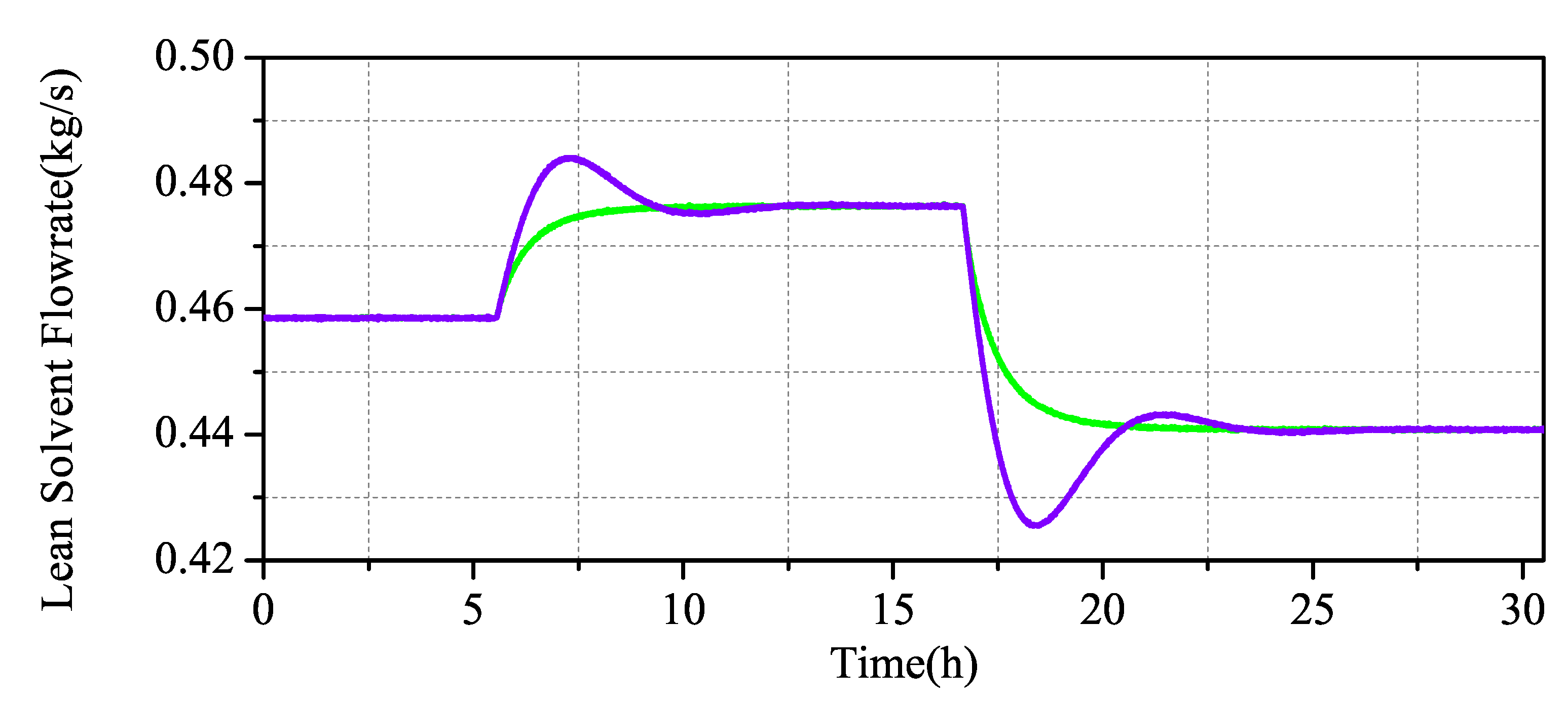
Figure 11.
Scenario 1: Comparison of MPC and PID simulation of the CO capture system.

Figure 12.
Scenario 2: (a) Comparison of MPC and PID simulation of controlled variables in CO capture; (b) zoom in current ramp-down at 1.4 h; (c) zoom in current ramp-up at 11.1 h; (d) zoom in current ramp-up at 23.6 h; and (e) Gaussian distributed random signal in the system.
Figure 12.
Scenario 2: (a) Comparison of MPC and PID simulation of controlled variables in CO capture; (b) zoom in current ramp-down at 1.4 h; (c) zoom in current ramp-up at 11.1 h; (d) zoom in current ramp-up at 23.6 h; and (e) Gaussian distributed random signal in the system.

Figure 13.
Scenario 2: Comparison of MPC and PID simulation of the CO capture system.


Table 1.
Flue gas condition.
| Property | Value | |
|---|---|---|
| Mole fraction | CO fraction HO fraction N fraction | 0.175 0.025 0.8 |
| Inlet gas flow rate/kg/s | 0.13 | |
| Temperature/K | 333 | |
| CO molar flowrate/kmol/s | 2.233 ×10 | |
Table 2.
Absorber/stripper parameters.
| Property | Absorber | Stripper |
|---|---|---|
| Pressure/kPa | 120 | 200 |
| Pressure drop/kPa | 10 | 10 |
| Equilibrium series | 20 | 20 |
| Packing Type | IMTP#40 | |
| Packing height/m | 6.1 | |
| Column internal diameter/m | 0.43 | |
Table 3.
Identification model of the post-combustion CO2 capture process.
| Object | A | B | C | D |
|---|---|---|---|---|
| Lean Solvent Flowrate to Capture rate | ||||
| Inlet Flue Gas to Capture rate |
Table 4.
Control parameters.
| Controller Type | Key Parameters |
|---|---|
| PID | = 1.5 = 0.2 = 0 |
| MPC | = 0.56 = 20 = 36 = 20 = 5 |
Table 5.
Step 1 performance indicators.
| Control Type | RT(s) | OS (%) | ST(s) | ITAE |
|---|---|---|---|---|
| MPC | 6709.50 | 0 | 2.7793 × | 6.0134 × |
| PID | 4600.763 | 16.47 | 3.7053 × | 1.2052 × |
Publisher’s Note: MDPI stays neutral with regard to jurisdictional claims in published maps and institutional affiliations. |
© 2021 by the authors. Licensee MDPI, Basel, Switzerland. This article is an open access article distributed under the terms and conditions of the Creative Commons Attribution (CC BY) license (http://creativecommons.org/licenses/by/4.0/).
Share and Cite
MDPI and ACS Style
Li, Q.; Zhang, W.; Qin, Y.; An, A. Model Predictive Control for the Process of MEA Absorption of CO2 Based on the Data Identification Model. Processes 2021, 9, 183. https://doi.org/10.3390/pr9010183
AMA Style
Li Q, Zhang W, Qin Y, An A. Model Predictive Control for the Process of MEA Absorption of CO2 Based on the Data Identification Model. Processes. 2021; 9(1):183. https://doi.org/10.3390/pr9010183
Chicago/Turabian StyleLi, Qianrong, Wenzhao Zhang, Yuwei Qin, and Aimin An. 2021. "Model Predictive Control for the Process of MEA Absorption of CO2 Based on the Data Identification Model" Processes 9, no. 1: 183. https://doi.org/10.3390/pr9010183
Note that from the first issue of 2016, this journal uses article numbers instead of page numbers. See further details here.