Differential Entropy Feature Signal Extraction Based on Activation Mode and Its Recognition in Convolutional Gated Recurrent Unit Network

Introduction

Signal recognition plays an important role in BCI devices [1]. The ability of perceived robots for expressing similar human behaviors is considered to be more approachable and humanized, which can obtain higher participation and more pleasant interaction in reality [2]. In recent years, an increasing number of researchers are attracted to the research of signal recognitions by computers. Electroencephalogram (EEG) signals can avoid the camouflage and subjectivity of human behaviors [3]. Therefore, feature signal recognition based on BCI devices is becoming a research focus.

At present, there are two technical problems in the process of feature signal recognition based on BCI devices. One is how to extract distinctive feature signals from original signals, and the other is how to establish a more effective feature recognition calculation model [4, 5]. Fast Fourier transform (FFT) was a common method to extract feature signals from the original signal [6]. However, FFT cannot reflect temporal information in frequency signal, so a short-time Fourier transform was used to extract time-frequency domain features which were recognized as a feature signal [7]. Human brain is a nonlinear dynamic system. It is difficult to analyze the original signal by traditional time-frequency feature extraction and analysis methods. So, by calculating the DE of the original signal, the differential asymmetry and rational asymmetry signals of the symmetrical electrodes in the left and right hemispheres of a brain were used for feature signal recognition, which achieved an average recognition accuracy of 69.67% on the DEAP dataset [8]. However, this could only explore the relationship between symmetric electrodes, not connect all electrodes in a spatial position. Recent research has shown that distinctive feature signals were closely related to multiple areas of the cerebral cortex in BCI [9]. The weights of brain areas were calculated by attention mechanism and the sum of weights was taken as the contribution value of brain areas, which showed that frontal lobe areas play an important role in feature signal recognition experiments [5]. The feature signals of different activation areas were extracted by DE and PSD topographic distribution, which found that prefrontal and temporal lobes of the cerebral cortex were related to feature signal states [10]. However, they did not use the relevant brain areas to improve the recognition rate of feature signals. Hence, a feature extraction method of multivariate empirical mode decomposition (MEMD) was used to select feature signal of appropriate channels, which achieved 75.00% on arousal and 72.87% on valence for feature signal recognition based on an Artificial Neural Network (ANN) classifier [11]. However, the traditional machine learning model is unable to extract more subtle feature signals, which could lead to a low performance of feature signal recognition. In recent years, feature signal recognition methods based on deep learning have developed rapidly. Especially, CNN model has become a leading method to improve recognition performance. A method of feeding time-frequency features of each channel into a 2DCNN model for feature signal state recognition was proposed, which achieved 78.12% on arousal and 81.25% on valence [12]. The original signal was decomposed into time frames, and the multi-channel time frame signals were used as inputs of a 3DCNN model, which achieved a recognition accuracy of 88.49% on arousal and 87.44% on valence [13]. The frequency domain feature, spatial feature and frequency band features of fusion multi-channel signals were fed into a Capsule Network (CapsNet) based on CNN, which achieved 68.28% on arousal and 66.73% on valence [14]. Although the CNN model can effectively extract the spatial information from feature signals, it cannot effectively extract the temporal information. Therefore, a hybrid neural network model combined CNN and Recurrent Neural Network (RNN) was proposed [15]. They used CNN model to extract the correlation of signals in physical adjacent channels, and used RNN model to mine the context information of feature signal sequences, which achieved 74.12% on arousal and 72.06% on valence. A Stack AutoEncoder (SAE) was used to establish a linear mixed model, and a long-short-term memory recurrent neural network (LSTM-RNN) was used for feature signal recognition, which could achieve 81.10% on arousal and 74.38% on valence. However, the unidirectional RNN and LSTM cannot backward learn the feature signal sequences, which was the reason of a low recognition rate.

For solving existing problems in previous studies, firstly, considering that different areas played different roles in feature signal recognition, activation pattern was introduced to reflect the weight of region contribution. So, a method of the DE feature signal extraction based on an activation mode was proposed. Secondly, a 1D and 3D feature signal representation method of considering the spatial-temporal information were also proposed, which could improve the recognition rate of feature signals by utilizing the temporal information of different areas and spatial connection of electrode positions. Lastly, a recognition framework based on Convolutional Gated Recurrent Unit network were proposed in this paper. The recognition framework was composed of 2DCNN and BiGRU in parallel, which could not only learn more distinctive and robust feature signals but also improve the recognition rate.

Methodlogy

DE Feature Signal Extraction

Original signals collected by the BCI include rhythm signals, event-related potentials, and spontaneous potential activity signals [4]. A Butterworth filter [16] is used to decompose the original signal (X) into four frequency band signals: X_θ, X_α, X_β, and, X_γ where θ is 4–7 Hz, α is 8–13 Hz, β is 14–30 Hz, and γ is 31–45 Hz.

DE Algorithm

DE is suitable for decoding characteristic signals [7, 10]. Each frequency band signal is divided into $X_i/\tau$ equal parts by a time window τ, and then analyzed by a DE algorithm. DE can discretize the value of continuous random variables. The signal sequence values are divided into small parts with ∆x. According to the mean value theorem, there is always a value x_i in each part to make Eq. 1 true.

where p(x_i) is a probability density function of discrete signals. Each point at i is assigned to x_i, and then the Eq. 1 is substituted into the Shannon formula for the discrete variables. The process is shown in Eq. 2.

When $△x$ approaches 0, ${\displaystyle {\sum }_{i=1}^{n}p\left(x_i\right)△x}$ approaches 1 and $\ln △x$ approaches −∞. So, the right side of the Eq. 2 approaches ∞, and the left side of Eq. 2 is seen as the DE of a continuous signal in Eq. 2. The DE can be defined as Eq. 3.

where X is a random variable, f(x) is a probability density function of X. Assuming that the original signal X obeys normal distribution $N\left(\mu ,\mathit{ }{\sigma }^2\right)$, the DE can be solved as Eq. 4.

where μ is a mean of X, and σ² is a variance of X. In Eq. 4, the DE of signal source X_i can be calculated as long as σ² is known, and the variance of normal distribution $N\left(\mu ,\mathit{ }{\sigma }^2\right)$ can be calculated via Eq. 5.

The spectral energy of the discrete signal is defined as $P={\displaystyle {\int }_{-\infty }^{+\infty }{f}^2\left(t\right)}\mathrm{ }dt$. According to Eq. 5, the variance of signal source X_i is an average spectral energy value P. From Eq. 4, the variance of X_i is a constant multiple $\left(P_i/N^2\right)$ of the spectral energy in each frequency band. So, the DE of a specific frequency band can be defined as Eq. 6.

where $H_i\left(X\right)$ is the DE of X_i , P_i is a spectral energy of X_i , σ_i² is a variance of X_i , and N is a constant.

DE Feature Signal Vector

A distinctive feature vector is constructed by using $H_i\left(X\right)$, the processing process for a baseline signal of a specific frequency band can be expressed as Eq. 7.

Where t is a total signal time, τ is a time sliding window, $v_j^i$ is the final DE feature vector at jth segment of ith band, $v_{trail}^i\left(j\right)$ is a DE feature vector at jth segment of ith frequency band, $v_{base}^i\left(k\right)$ is a DE feature vector of a baseline signal in jth segment of ith band, and m is a number of segments in baseline signals. So, a 1D DE feature signal vector can be expressed as $v_j^i={\left[c_{\tau }^1,\mathrm{ }{c}_{\tau }^2,\mathrm{ }\mathrm{...}\mathrm{ },c_{\tau }^n\right]}^T\in R^n$, where n is the number of electrode channels, $c_j^n$ is the pre-processed signal at nth channel of jth segment.

The 1D data of n channels are filled into the space electrode position of d×d, and the unused electrode position is filled with zero value. Then, a 2D matrix (f_τ) can be obtained. In order to make the matrix denser, a radial basis function (RBF) interpolation of Gaussian kernel function [17] is used to fill in zero values. This process can be expressed as Eq. 8.

Where σ is an extension constant of the RBF function, x is a center point, c is an electrode channel point, and $\Vert \cdot \Vert$ is 2-norm.

Convolutional Gated Recurrent Unit Network

The convolutional gated recurrent unit network is composed of 2DCNN and BiGRU in parallel, as shown in Figure 1.

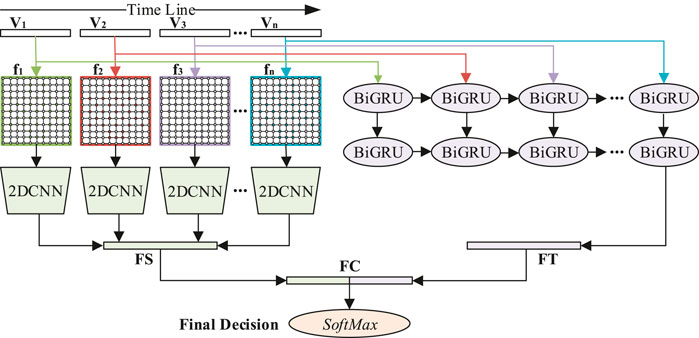
FIGURE 1. Schematic diagram of DE feature signal recognition model based on 2DCNN-BiGRU. The 1D feature sequences of each time step are fed into BiGRU to extract the time information of feature signals. The 2D feature matrices of each time step are fed into 2DCNN to extract the spatial information of feature signals. Finally, the decision layer gives the recognition result.

Structural Principle of 2DCNN

CNN is a kind of forward feedback neural network. The model structure mainly includes input layers, hidden layers and output layers. The network structure of 2DCNN is shown in Figure 2. The feature signal matrix ${\stackrel{\mathrm{ }\mathbf{\wedge }}{\mathbf{f}}}_{\tau }\left(c\right)$ is used as the input of 2DCNN. The abstract feature extraction of the DE feature signal is completed by setting the size of the 2D filters, the process can be defined as Eq. 9.

where W is the convolution kernel, (m, n) is the size of the convolution kernel W, ${\stackrel{\mathrm{ }\mathbf{\wedge }}{\mathbf{f}}}_{\tau }$ is the input matrix, (i, j) is the matrix coordinate. After each convolution operation, the feature data of each layer is batch-normalized (BN), and a RELU activation function is added to make the model have nonlinear feature transformation capability. The RELU function is expressed as Eq. 10.

where max is the maximum function, x is the inputs. The feature matrix S is fed into the fully connected layer to make it more expressive in space. The process is shown as Eq. 11.

where R¹⁰¹⁴ represents a dimension of 1,024, FC is the fully connection layer, and FS is a 1,024-dimensional vector.

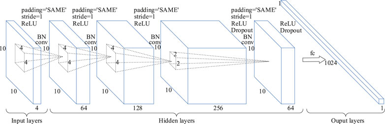
FIGURE 2. Schematic diagram of the 2DCNN model. The inputs are a 3D DE feature matrix of 10 × 10 × 4, and its construction process is shown in Construction of 3D DE Feature Matrix section. Padding = ‘SAME’ represents the edge information is filled with zeros, Stride = 1 means that the step size of each convolution operation is 1, and Dropout means that hidden neurons are deleted randomly.

Structural Principle of BiGRU

GRU [18] is an improvement of LSTM [19]. Compared with LSTM, GRU is capacity of dealing with a smaller amount of data, which has a faster calculation speed and can better solve the problem of gradient disappearance. The schematic diagram of GRU is shown in Figure 3A. The GRU processes sequence information by resetting gate r_z and updating gate z_t, and its parameter update equation is shown in Eqs. 12–15.

where w_r, w_z, w_h, U_r, U_z, and U_h are the weight parameters of the BiGRU network, r_t is reset gate, z_t is update gate, ${\tilde{h}}_t$ is candidate activation unit, h_t is the hidden unit at time t, h_t-1 is the hidden unit at time t−1, σ is the activation function, V_t is the GRU input at time t, ⊗ represents multiplying by elements, and ⊕ represents adding by elements.

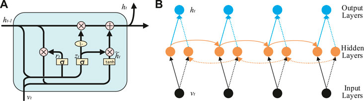
FIGURE 3. (A) Schematic diagram of GRU network. (B) Schematic diagram of BiGRU network.

DE feature matrix V is exploited to be the original input of BiGRU network. The BiGRU network is composed of forward GRU, backward GRU, and forward-backward output state connection layers. The structure of BiGRU network is shown in Figure 3B, which mainly includes input layers, hidden layers and output layers.

Experimental Results and Discussion

In this part, the experimental processes would be introduced and our method would be compared with other methods. Then, the effectiveness of our framework was evaluated on the DEAP dataset. To achieve a more reliable emotion recognition process, the emotion recognition performance of the EEG access was analyzed by a 5-fold cross-validation technology.

Experimental Environment and Experimental Dataset

Table 1 Shows the specific experimental environment for experiments.

TABLE 1. Specific experimental environment.

In the DEAP dataset [4], EEG signals of 32 subjects who watched 40 1-minute music videos were recorded, and each subject contained 63s EEG data of 32 electrode channels. Among them, the first 3s was the baseline signal recorded in the relaxed state, and the last 60s was the trial signal recorded when watching the videos.

According to the level of arousal and valence, the distinctive categories of DE feature signal states were obtained. In our experiment, the DE feature signal recognition was divided into two binary classifications. If scores of the arousal or valence were less than or equal to 5, the label was marked as low. If scores were greater than 5, the label was marked as high. Thus, there were four labels on arousal and valence: high arousal (HA), low arousal (LA), high valence (HV) and low valence (LV).

Data Preprocessing

In order to improve the accuracy of recognition, the influence of baseline signals on trial signals needs to be considered. Before extracting the DE feature signal of original signals, the original signals are usually divided into short time frames [15, 19, 20]. The baseline signal was divided into three segments with a 1s sliding window and the trial signal into $n=60/\tau$ segments with a τwindow. As shown in Figure 4, a channel signal of the original data was taken out, and the original signal of each second is decomposed into θwave, αwave, βwave, and γwave through the Butterworth filters. The DE vectors Base_Vector (i) of the three baseline signals and the DE vectors Trail_Vector (n) of the trial signals in each time window were calculated by the DE algorithm. Then, n-feature signals ($\mathrm{D}{\mathrm{E}}_{i=\theta ,\alpha ,\beta ,\gamma }^1$) in this channel could be obtained by Trail_Vector (n) minus Mean∑_i=1,2,3 Base_Vector (i) in turn. Finally, the 1D vector $D{E}_i=\left[D{E}_i^1,\mathrm{ }D{E}_i^1,\mathrm{ }\mathrm{...}\mathrm{ },\mathrm{ }D{E}_i^{32}\right]$ of 32 electrode channels could be obtained, where i is the frequency band.

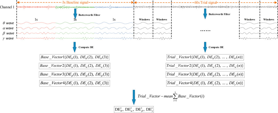
FIGURE 4. Schematic diagram of the original signal preprocessing flow. Among them, Trail_Vector (n) is the baseline signal feature vector. Trail_Vector (n) is the trial signal feature vector. $D{E}_i=\left[D{E}_i^1,\mathrm{ }D{E}_i^1,\mathrm{ }\mathrm{...}\mathrm{ },\mathrm{ }D{E}_i^{32}\right]$ is the DE feature signal vector of 32 channels. Mean ∑ Base_Vector (i) is the sum average DE of three baseline segmentations.

Construction of 3D DE Feature Matrix.

The DE feature signal value of 32 channels was filled to the orange position in Figure 5B, and the gray point was filled with zero values. The electrodes circled in orange were the test points used in the DEAP dataset, as shown in Figure 5A. The electrodes of the international 10–20 system [10] were connected with the test electrodes of the DEAP dataset, which could construct a square matrix N × N (N is the maximum number of points between the horizontal test points and the vertical test points). In addition, in order to avoid the loss of edge information, a layer of gray unused points was added to the outer layer of the matrix, as shown in Figure 5B. In order to make the matrix denser, the RBF interpolation was used to fill in the zero values [17]. Finally, a 3D feature matrix was obtained by stacking the 2D feature matrices of four frequency bands, as shown in Figure 5C.

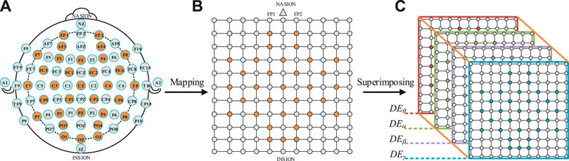
FIGURE 5. Schematic diagram of a 3D feature signal matrix construction. (A) International 10–20 system [10]. (B) A 2D square matrix of 32 EEG channels. (C) A 3D feature matrix of DE_θ, DE_α, DE_β and DE_γ.

The sliding windows of 1, 10, 30 and 60s were used to divide the original signals, and the number of DE feature signal samples obtained is shown in Table 2. Notably, the time step window of 60s was the original signal length. The total samples of each frequency band were 32 × 40 × n, where 32 was the number of subjects, 40 was the number of experiments of each subject, and n was the number of signals divided by the time window. Finally, the same number of samples of the 1D feature signal vectors and 2D feature signal matrices of each frequency band were obtained.

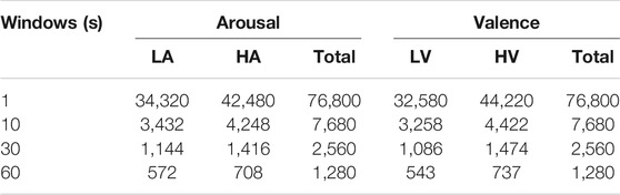
TABLE 2. The number of feature signal samples of each frequency band signal at 1, 10, 30, and 60s time windows.

2DCNN-BiGRU Model Training and Parameter Setting

The 1D feature signal vectors and 3D feature signal matrices were fed into BiGRU model and 2DCNN model respectively. The proposed model was implemented with Tensorflow framework and trained on an NVIDIA GeForce RTX 2060 GPU. The Adam optimizer was adopted to minimize the cross-entropy loss function. The keep probability of dropout operation was 0.5. The penalty strength of L2 was 0.5. The hidden sates of the GRU cell is the number of channels. The learning rate was initialized to 0.001. When the verification errors of the model stopped dropping, the learning rate was divided by 10 until the iteration stopped.

In the 2DCNN model of the first three convolutional layers, 64, 256, and 512 convolution kernels with a size of 4 × 4 were used respectively. In order to reduce the amount of calculation, 64 convolution cores with a size of 2 × 2 were used in the fourth convolution layer, which added a dropout operation. In addition, in each convolutional layer, stride was set to 1, padding was set to SAME, and zero padding was used to prevent information from being lost at the edge of the inputs. A fully connected layer was used to convert input features into spatial abstract features. In order to avoid learning overfitting and improve the generalization ability of the model, L2 regularization was added to the network. And then, two layers BiGRU were used to fused the temporal features obtained by the BiGRU model with the spatial features obtained by the 2DCNN model. Finally, the DE feature signal recognition result was obtained through a SoftMax classifier.

Results of 2DCNN-BiGRU in All Electrode Channels

The 5-fold cross-validation technology was used to validate all subjects and the recognition results of θ frequency band, α band signal, β frequency band signal, γ band signal and four band signal combinations were counted at four-time windows. The recognition results were shown in Table 3. In the dimensions of arousal and valence, the high frequency band (β and γ) had higher average recognition accuracy than the low frequency band (θ and α), which showed that the high frequency band had more abundant DE feature signal information. It also could be observed that the accuracy of all band combinations was higher than a single band. The 2DCNN-BiGRU model achieved the highest average recognition accuracy of 87.20 and 87.90% on arousal and valence at the 10s sliding window.

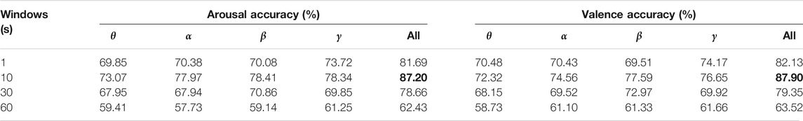
TABLE 3. When the inputs of the 2DCNN-BiGRU model were data of 32 electrodes, the DE feature signal recognition results of each frequency band signal and all frequency band combinations under the time window of 1, 10, 30, and 60s, respectively.

Results of DE Feature Signal Recognition in Activation Mode

In order to explore the influence of electrode channels on the recognition rate of DE feature signals, the activation model of DE feature signals and PSD feature signals were studied [19]. The DE feature signals were classified by reducing the electrode channels under the activation model. A brief framework for the recognition process is shown in Figure 6.

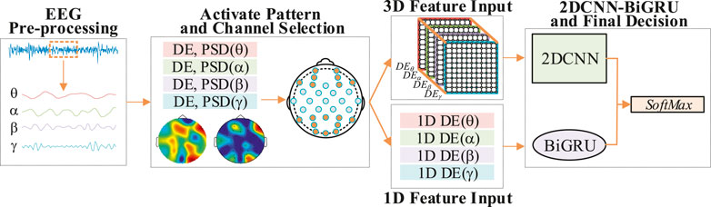
FIGURE 6. A brief frame diagram of DE feature signal recognition of convolutional gated recurrent network based on activation mode.

In the DEAP dataset, the average value of DE and PSD were calculated, which were from the 32 electrode channels of all subjects at different time windows. Figure 7A and Figure 7B showed the averaged PSD and DE distribution, where four frequency bands (theta, alpha, beta and gamma) represented four activation models. It was found that the electrode channels located in the frontal and occipital lobes had a higher activation capacity. However, different time windows have similar activation patterns on different frequency bands, which is the reason for the lower recognition accuracy of DE feature signals. The activation ability of high frequency bands (beta and gamma) is greater than that of low frequency band (theta and alpha), which also explains that beta and gamma bands have better recognition effect than theta and alpha bands. According to the spatial locations of the electrodes, the 32 electrodes used in the DEAP dataset were divided into five clusters, namely, five brain areas, as shown in Figure 8A. Table 4 summaries the electrode channels in each brain region, where the frontal lobe represents the electrodes of FP1, AF3, F7, F3, FP2, AF4, F8, F4, and FZ, the central lobe represents the electrodes of FC1, CP1, C3, FC2, CP2, C4, and CZ, the temporal lobe represents the electrodes of FC5, T7, CP5, FC6, T8, and CP6, the parietal lobe represents the electrodes of P7, P3, P8, P4, and PZ, and the occipital lobe represents the electrodes of PO3, O1, PO4, O2, and OZ.

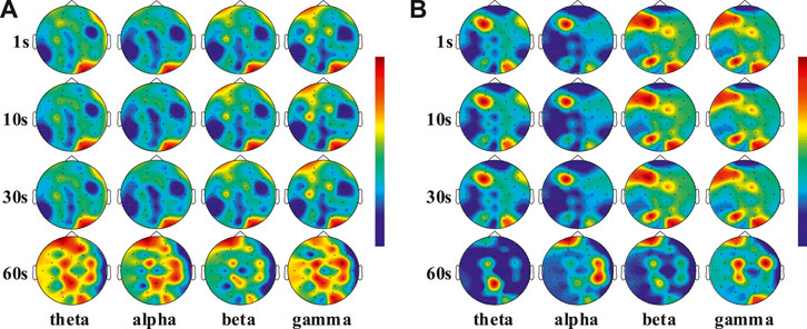
FIGURE 7. (A) Scalp distribution of the DE feature signal at 1, 10, 30, and 60s windows of different frequency bands. (B) Scalp distribution of the PSD feature signal at 1, 10, 30, and 60s windows of different frequency bands.

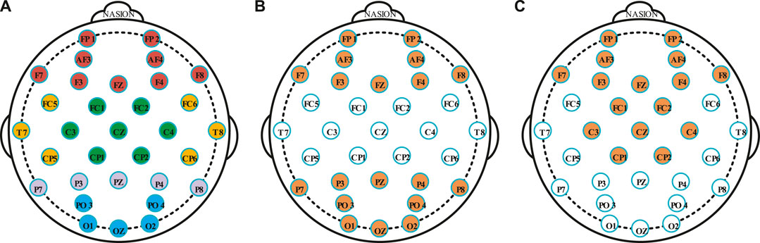
FIGURE 8. (A) The 32 electrodes of the DEAP dataset are divided into five groups, and the same color represents the same group of areas. (B) The 19 electrodes are selected by the activation modes at the 1, 10, and 30s windows. (C) The 16 electrodes are selected by the activation modes at the 60s windows.

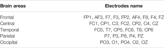
TABLE 4. The 32 electrodes in the DEAP dataset are divided into five areas and the electrodes represents by each brain area.

According to the activation areas of each time window, the combinations of different areas were selected. As shown in Figure 8B, the frontal, parietal, and occipital areas were considered as the DE feature signal activation areas at 1, 10, and 30s windows. The number of electrodes were reduced from 32 to 19, where the selected electrodes were FP1, AF3, F7, F3, FP2, AF4, F8, F4, FZ, P7, P3, P8, P4, PZ, PO3, O1, PO4, O2, and OZ. Under the 60s-time step window, the frontal lobe and central area were used as the activation areas of the DE feature signals, as shown in Figure 8C. The number of electrodes were reduced from 32 to 16, and the selected electrodes were FP1, AF3, F7, F3, FP2, AF4, F8, F4, FZ, FC1, CP1, C3, FC2, CP2, C4, and CZ.

The DE feature signals of the four frequency bands were used as the inputs of the 2DCNN-BiGRU model, and the DE feature signal recognition experiments with the selected electrode were performed at each time window. The recognition results were shown in Figure 9. At 1s window, the recognition rate of 19 electrodes improved by 0.06% on valence compared with 32 electrodes, while decreased by 0.69% on arousal. At 10s window, the recognition rate of 19 electrodes improved by 0.79% on arousal and 0.06% on valence compared with 32 electrodes. At 30 s window, the recognition rate of 19 electrodes decreased by 0.77% on arousal and 1.21% on valence compared with 32 electrodes. At 60 s window, the recognition rate of 16 electrodes improved by 0.04% on arousal and 0.19% on valence compared with 32 electrodes. Notably, when the time window was 10 s, the 2DCNN-BiGRU model achieves the highest accuracy. Experimental results showed that there were different activation modes at different time scales. By reducing the number of electrodes in the activation mode, not only could achieve the recognition rate which was similar to all electrodes of DE feature signal recognition, but also the performance and robustness of the recognition models could be improved.

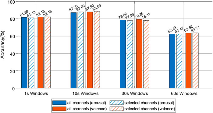
FIGURE 9. DE feature signal recognition results of 2DCNN-BiGRU in activation mode.

In order to further verify the reduction of electrode channels could achieve similar accuracy to all electrodes, and to verify that the hybrid model is better than the single model, four models of 2DCNN, BiLSTM, BiGRU, and 2DCNN-BiLSTM are compared with the 2DCNN-BiGRU. Table 5 shows the structure and inputs of different models.

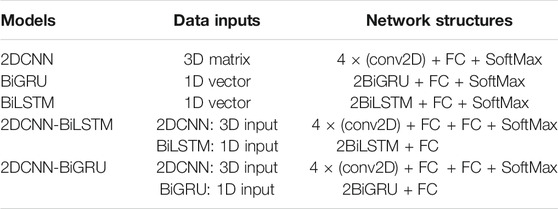
TABLE 5. The structure and inputs of 2DCNN, BiLSTM, BiGRU, 2DCNN-BiLSTM, and 2DCNN-BiGRU models.

In the experiment, the data of the 10s window were used as the inputs of the models, and the sum average of arousal and valence as the final results. In order to make the experiment comparable, the convolutional kernels of each model and the fully connected layer parameter settings were consistent in experiments. The DE feature signal recognition rate of each model was shown in Figure 10. The recognition rate of the selected electrodes was slightly higher than that of all electrodes in different models. The recognition rate of 2DCNN-BiLSTM and 2DCNN-BiGRU is higher than that of 2DCNN, BiLSTM and BiGRU, which indicated that the hybrid models could effectively extract the spatial-temporal features of DE feature signals. The recognition rate of the 2DCNN-BiGRU model was slightly higher than that of the 2DCNN-BiLSTM model, which indicated that the GRU unit was superior to the LSTM unit in handling small samples.

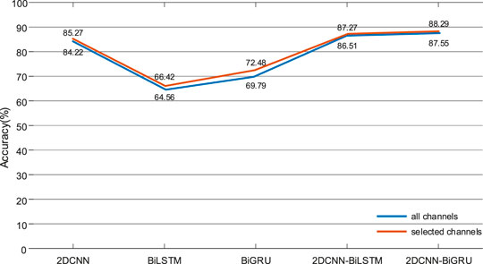
FIGURE 10. At the 10s windows, the DE feature signal recognition results of 2DCNN, BiLSTM, BiGRU, 2DCNN-BiLSTM, and 2DCNN-BiGRU in the activation mode.

Comparison of the results of different experimental methods.

The proposed method was compared with the current recognition methods based on feature signals, which were applied to the DEAP dataset. As shown in Table 6, the binary classification experiments of valence and arousal were carried out, and the similar methods were followed to evaluate the recognition accuracy.

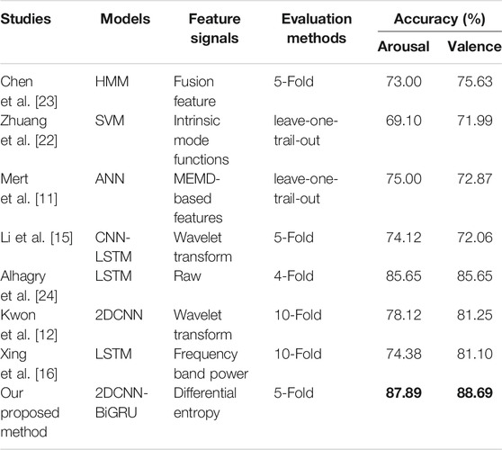
TABLE 6. Comparison of the different experimental methods in the DEAP dataset.

Our model was compared with traditional machine learning models of HMM [21], SVM [22] and ANN [11], as shown in Figure 11. The accuracy of our method improved by 12.89% on arousal and 13.06% on valence, which showed that the DE feature signal recognition based on deep learning method could deeply extract more subtle abstract features and achieve higher recognition rate.

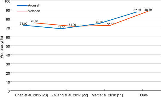
FIGURE 11. The proposed method is compared with the traditional machine learning methods.

In order to further verify the effectiveness of the proposed method, the 2DCNN-BiGRU model was compared with the latest deep learning methods, such as 2DCNN [12], LSTM [19, 23] and CNN-LSTM [15], as shown in Figure 12. Compared with the 2DCNN model, our model improved by 9.77% on arousal and 7.44% on valence, which indicated that BiGRU could handle the dynamic information of deep feature signal sequences. Compared with the LSTM model, our model improved by 2.24% on arousal and 3.04% on valence, which indicated that the 2DCNN model could effectively extract the spatial feature. Compared with the CNN-LSTM model, our model improved by 13.77% on arousal and 16.63% on valence, which indicated that our spatial-temporal features based on the activation modes are more effective. In addition, the DE feature signal was compared with wavelet transform (WT) [12, 15] power spectral density (PSD) [19] and raw signals [24], which showed that the DE feature signals are more effective in our model. However, on one hand, the hybrid 2DCNN-BiGRU model contains massive amounts of parameters, which is necessarily unfriendly to hardware devices. On the other hand, a more advanced Graph Convolution Network (GCN) [23, 25] can be considered to further explain the relationship between the electrodes.

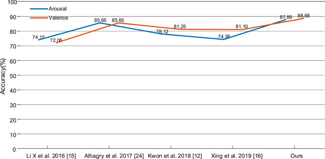
FIGURE 12. The proposed method is compared with other deep learning methods.

Conclusion

In this paper, a DE feature signal extraction method based on an activation mode and its recognition in a Convolutional Gated Recurrent Unit network were proposed. The DE and PSD feature signals were used to mine activation patterns at different time scales to reduce electrode channels. The 1D temporal and 3D spatial feature signals were respectively fed into 2DCNN and BiGRU models, which achieved a recognition accuracy of 87.89% on arousal and 88.69% on valence of the DEAP dataset. It was found that DE feature signals of reducing electrode channels could achieve similar recognition accuracy to all electrode channels, which was of great significance to develop a recognition device based on BCI system.

Data Availability Statement

Publicly available datasets were analyzed in this study. This data can be found here: http://www.eecs.qmul.ac.uk/mmv/datasets/deap/index.html.

Author Contributions

YZ designed the framework, conducted experiments and wrote the manuscript. QZ carried out experiments and analyzed the results and presented the discussion and conclusion parts.

Funding

This research was funded by the National Natural Science Foundation of China (No. 61871433), the Natural Science Foundation of Guangdong Province (No. 2019A1515011940), the Science and Technology Program of Guangzhou (Nos. 202002030353 and 2019050001), the Science and Technology Planning Project of Guangdong Province (Nos. 2017B030308009 and 2017KZ010101), the Guangdong Provincial Key Laboratory of Optical Information Materials and Technology (No. 2017B030301007), and the Guangzhou Key Laboratory of Electronic Paper Displays Materials and Devices.

Conflict of Interest

The authors declare that the research was conducted in the absence of any commercial or financial relationships that could be construed as a potential conflict of interest.

References

1. Korovesis N, Kandris D, Koulouras G, Alexandridis A. Robot motion control via an EEG-based brain–computer interface by using neural networks and alpha brainwaves. Electronics (2019) 8(12):1387–1402. doi:10.3390/electronics8121387
2. Xiao G, Ma Y, Liu C, Jiang D. A machine emotion transfer model for intelligent human-machine interaction based on group division. Mech Syst Signal Process (2020) 142:106736–850. doi:10.1016/j.ymssp.2020.106736
3. Hu B, Li X, Sun S, Ratcliffe M. Attention recognition in EEG-based affective learning research using CFS+KNN algorithm. IEEE/ACM Trans Comput Biol Bioinf (2018) 15(1):38–45. doi:10.1109/tcbb.2016.2616395
4. Koelstra S, Muhl C, Soleymani M, Lee J-S, Yazdani A, Ebrahimi T, et al. DEAP: a database for emotion analysis; using physiological signals. IEEE Trans Affective Comput (2012) 3(1):18–31. doi:10.1109/t-affc.2011.15
5. Li Y, Zheng W, Wang L, Zong Y, Cui Z. From regional to global brain: a novel hierarchical spatial-temporal neural network model for EEG emotion recognition. IEEE Trans Affective Comput (2019) 99:1. doi:10.1109/taffc.2019.2922912
6. Yin Z, Wang Y, Liu L, Zhang W, Zhang J. Cross-subject EEG feature selection for emotion recognition using transfer recursive feature elimination. Front Neurorobot (2017) 11:19. doi:10.3389/fnbot.2017.00019
7. Liu YJ, Yu M, Zhao G, Song J, Ge Y, Shi Y. Real-time movie-induced discrete emotion recognition from EEG signals. IEEE Trans Affective Comput (2018) 9(4):550–62. doi:10.1109/taffc.2017.2660485
8. Zheng WL, Zhu JY, Lu BL. Identifying stable patterns over time for emotion recognition from EEG. IEEE Trans Affective Comput (2019) 10(3):417–29. doi:10.1109/taffc.2017.2712143
9. Zhong Q, Zhu Y, Cai D. Electroencephalogram access for emotion recognition based on deep hybrid network. Front Hum Neurosci (2020) 14:1–13. doi:10.3389/fnhum.2020.589001
10. Li P, Liu H, Si Y, Li C, Li F, Zhu X, et al. EEG based emotion recognition by combining functional connectivity network and local activations. IEEE Trans Biomed Eng (2019) 66(10):2869–81. doi:10.1109/tbme.2019.2897651
11. Mert A, Akan A. Emotion recognition from EEG signals by using multivariate empirical mode decomposition. Pattern Anal Appl (2016) 21(1):81–9. doi:10.1007/s10044-016-0567-6
12. Kwon YH, Shin SB, Kim SD. Electroencephalography based fusion two-dimensional (2D)-convolution neural networks (CNN) model for emotion recognition system. Sensors (2018) 18(5):1383–95. doi:10.3390/s18051383
13. Salama ES, El-Khoribi RA, Shoman ME, Shalaby MAW. EEG-based emotion recognition using 3D convolutional neural networks. Int J Adv Comput Sci Appl (2018) 9(8). doi:10.14569/IJACSA.2018.090843
14. Chao H, Dong L, Liu Y, Lu B. Emotion recognition from multiband EEG signals using CapsNet. Sensors (2019) 19(9):2212. doi:10.3390/s19092212
15. Li X, Song D, Zhang P, Yu G, Hou Y, Hu B. Emotion recognition from multi-channel EEG data through convolutional recurrent neural network. IEEE Int Conf Bioinform Biomed (2016) 1:352–9. doi:10.1109/bibm.2016.7822545
16. Mahata S, Saha SK, Kar R, Mandal D. Optimal design of fractional order low pass Butterworth filter with accurate magnitude response. Digital Signal Process (2018) 72:96–114. doi:10.1016/j.dsp.2017.10.001
17. Cho J, Hwang H. Spatio-temporal representation of an electoencephalogram for emotion recognition using a three-dimensional convolutional neural network. Sensors (2020) 20(12):3491–508. doi:10.3390/s20123491
18. Cho K, Van Merrienboer B, Gulcehre C, Bahdanau D, Bougares F, Schwenk H. Learning phrase representations using rnn encoder-decoder for statistical machine translation. Comput Sci (2014) 2014: 1724–34. doi:10.3115/v1/D14-1179
19. Xing X, Li Z, Xu T, Shu L, Hu B, Xu X. SAE+LSTM: a new framework for emotion recognition from multi-channel EEG. Front Neurorobot (2019) 13:37. doi:10.3389/fnbot.2019.00037
20. Wang XW, Nie D, Lu BL. Emotional state classification from EEG data using machine learning approach. Neurocomputing (2014) 129:94–106. doi:10.1016/j.neucom.2013.06.046
21. Chen J, Hu B, Xu L, Moore P, Su Y. Feature-level fusion of multimodal physiological signals for emotion recognition. IEEE Int Conf Bioinform Biomed (2015) 1:395–99. doi:10.1109/bibm.2015.7359713
22. Zhuang N, Zeng Y, Tong L, Zhang C, Zhang H, Yan B. Emotion recognition from EEG signals using multidimensional information in EMD domain. Biomed Res Int (2017) 2017:83173579. doi:10.1155/2017/8317357
23. Xiao L, Hu X, Chen Y, Xue Y, Gu D, Chen B, et al. Targeted sentiment classification based on attentional encoding and graph convolutional networks. Appl Sci (2020) 10(3):957–73. doi:10.3390/app10030957
24. Alhagry S, Fahmy AA, El-Khoribi RA. Emotion recognition based on EEG using LSTM recurrent neural network. Int J Adv Comput Sci Appl (2017) 8(10):355–8. doi:10.14569/IJACSA.2017.081046
Keywords: differential entropy, signal extraction, activation mode, convolutional neural network, bidirectional gated recurrent unit network
Citation: Zhu Y and Zhong Q (2021) Differential Entropy Feature Signal Extraction Based on Activation Mode and Its Recognition in Convolutional Gated Recurrent Unit Network. Front. Phys. 8:629620. doi: 10.3389/fphy.2020.629620
Received: 15 November 2020; Accepted: 04 December 2020;
Published: 18 January 2021.
Edited by:
Zichuan Yi, University of Electronic Science and Technology of China, ChinaReviewed by:
Congcong Ma, Nanyang Institute of Technology, ChinaJunsheng Mu, Beijing University of Posts and Telecommunications (BUPT), China
Guodong Liang, Jinan University, China
Copyright © 2021 Zhu and Zhong. This is an open-access article distributed under the terms of the Creative Commons Attribution License (CC BY). The use, distribution or reproduction in other forums is permitted, provided the original author(s) and the copyright owner(s) are credited and that the original publication in this journal is cited, in accordance with accepted academic practice. No use, distribution or reproduction is permitted which does not comply with these terms.
*Correspondence: Qinghua Zhong, zhongqinghua@m.scnu.edu.cn