Finding Optimal Stations Using Euclidean Distance and Adjustable Surrounding Sphere


1
Data & High Performance Computing Science, University of Science and Technology, Daejeon 34113, Korea
2
Korea Institute of Science and Technology Information, Daejeon 34141, Korea
3
Faculty of Informatics, Burapha University, Chon Buri 20131, Thailand
*
Authors to whom correspondence should be addressed.
Appl. Sci. 2021, 11(2), 848; https://doi.org/10.3390/app11020848
Submission received: 31 December 2020
/
Revised: 14 January 2021
/
Accepted: 15 January 2021
/
Published: 18 January 2021
(This article belongs to the Special Issue Advances in Air Quality Monitoring and Assessment)
Abstract
:Air quality monitoring network (AQMN) plays an important role in air pollution management. However, setting up an initial network in a city often lacks necessary information such as historical pollution and geographical data, which makes it challenging to establish an effective network. Meanwhile, cities with an existing one do not adequately represent spatial coverage of air pollution issues or face rapid urbanization where additional stations are needed. To resolve the two cases, we propose four methods for finding stations and constructing a network using Euclidean distance and the k-nearest neighbor algorithm, consisting of Euclidean Distance (ED), Fixed Surrounding Sphere (FSS), Euclidean Distance + Fixed Surrounding Sphere (ED + FSS), and Euclidean Distance + Adjustable Surrounding Sphere (ED + ASS). We introduce and apply a coverage percentage and weighted coverage degree for evaluating the results from our proposed methods. Our experiment result shows that ED + ASS is better than other methods for finding stations to enhance spatial coverage. In the case of setting up the initial networks, coverage percentages are improved up to 22%, 37%, and 56% compared with the existing network, and adding a station in the existing one improved up by 34%, 130%, and 39%, in Sejong, Bonn, and Bangkok cities, respectively. Our method depicts acceptable results and will be implemented as a guide for establishing a new network and can be a tool for improving spatial coverage of the existing network for future expansions in air monitoring.
1. Introduction
Air quality monitoring networks (AQMN) are established as tools that determine policies and strategies for achieving air quality standards. A plan for designing an AQMN depends on objectives such as urban planning, environmental policies, and budget. Generally, designing an AQMN is done by environmental authorities or governmental organizations based on empirical judgments. An expert group assesses various criteria to make their decisions, such as budget and population thresholds. These play a significant role in determining the required number and location of monitoring stations. For example, Thailand and South Korea set up air monitoring stations in government office areas to reduce the cost of installation, maintenance, and the safety of the devices [1,2]. Guidelines of the USA and Australia suggest installing new air quality monitoring stations based on population size [3,4]. In such cases, monitoring stations are often considered in an ad hoc fashion.
The critical issues in AQMN designing are separated into a setting up network for allocating optimum stations and optimizing the existing network to better reflect air quality in the area. There are different methods to design a new network, all of which must comply with the Environmental Protection Agency (EPA) guideline or local government regulations [5]. Furthermore, various studies mainly consider pollution data, population density, land-use regression, distance to major roads, and high-risk observation regions to identify new air quality monitoring stations [6,7,8,9,10]. Some studies investigated pollution indicators in the area surrounding stations [11,12,13]. Such a zone is called a sphere of influence (SOI) and the original algorithm was developed by Liu et al. in 1986. Their proposed method uses air pollution data to determine spatial coverage and the number of air monitoring stations [14].
Optimization, evaluation, and revision of existing AQMN to meet changing local area pollution levels has been an important research topic over the past few decades [15,16,17,18]. The main cause regarding the distribution of air pollution and emission source changed caused by urbanization. The rapid expansion of the urban areas in developing countries of Asia leads to air quality monitoring issues such as excessive numbers of stations in urban regions and a lack of adequate numbers of stations in rural areas [19]. Consequently, several approaches have suggested adding or removing stations by considering various constraints such as population density, historical pollution data, terrain conditions, budget, and health impact. They use statistical analytics, weight criteria, holistic approaches, data simulation, and pure measurement for AQMN optimization [20,21,22]. Moreover, some studies apply terrain maps, heat maps, gridded synthetic assessment, and graphical information systems (GIS) to show high pollution concentration areas. They analyze pollution criteria and combine them with spatial statistics to determine suitable areas to recommend for station location sites [23,24,25,26,27].
However, studies of optimal designs or revision of AQMN in less developed countries (LDCs) are relatively scarce. Such studies in the literature are mostly related to minimizing air pollution’s health impact [28,29]. The LDCs have different issues than in developed countries, such as limited budgets to establish the stations, lack of historical pollution data, and requirements that demand air pollution monitoring cover vast areas. All of these constraints are critical factors for AQMN design [30]. Therefore, recommending the station location to cover a prospective land use expansion has an important key role for sustainable development of air pollution control and helps assess air pollution’s spatial variability for better monitoring of air quality [31].
Previous studies attempted to design air monitoring networks by considering specific air pollution concentration, cost, population data, and other parameters, while spatial coverage was ignored. Such a design methodology causes station locations to have high density in some particular regions, especially in urban areas. It does not distribute coverage to rural areas with a sufficient number of stations. The incremental building of air quality monitoring in urban areas can make better monitoring of the specific areas. However, it leads to an increase in installation and maintenance costs, which is one of the main constraints for designing a dense air quality monitoring network. Furthermore, none of the methods in previous studies mentioned designing an AQMN without historical pollution data or city characteristics data. Furthermore, it is important to consider that the air monitoring networks designed are not only for use today but also for urban expansion in the future.
We organized the rest of the paper as follows. Problem formulation is introduced in Section 2. We describe the study areas in Section 3. In Section 4 proposes four methods for finding the best next station, which includes algorithms and equations. In Section 5, the evaluation criteria will be explained. The results of the proposed methods are compared and discussed in Section 6. Finally, Section 7 draws our conclusion and suggests possible future work.
2. Problem Formulation
The studied problem is based on finding the next stations to achieve maximum spatial coverage. We apply the concept of Euclidean Distance and the k-nearest neighbor algorithm (k-NN) to calculate the distance between station neighbors. The objectives are set up a network and improve an existing network. In the preparation process, we divide map of study areas into a square of a grid and identify latitude longitude pairs at the centroid of all grids. Such geographic coordinates are used to calculate the distance. Given only a study area map and a specified number of stations, how can one calculate and recommend the stations to achieve maximum spatial coverage? The objective is to find the stations which meet the following constraints:
- (i)
- Achieve maximum spatial coverage while maintaining proper overlapped area between the nearest-neighbors’ stations
- (ii)
- Propose methods without using historical pollution and city characteristics data.
The proposed method was tested and demonstrated in three real cities and compared with existing network coverage. This study can provide recommendations for environmental authorities or city planners to select the stations for increasing spatial coverage of air quality monitoring.
3. Study Areas
This study used three cities—Sejong: South Korea, Bangkok: Thailand, and Bonn: Germany—as the primary research areas. The three cities are developed smart city prototypes facing urban expansion shortly. Another reason for our choices is that the three regions have different sizes and shapes. The sizes of the cities in ascending order are Bonn, Sejong, and Bangkok, respectively. Because the size of Sejong is in the middle, we chose Sejong city as the primary implementation, and the other two cities are used as test cases. Our study areas are described in this section.
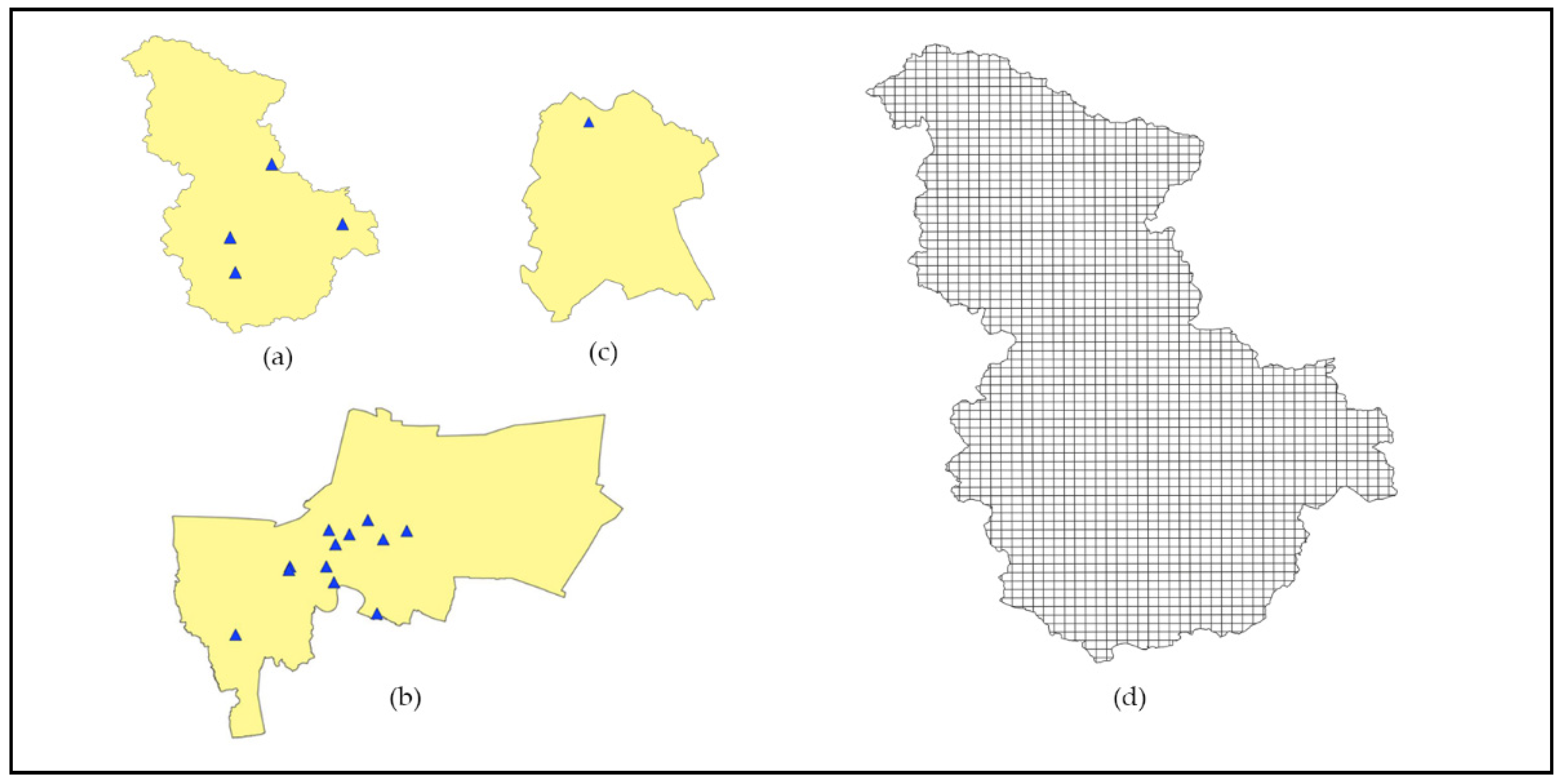
Sejong city is located almost the middle of Korea on a long, stretching mainly north to south. The population was about 350,000 in October 2020, and the size of Sejong city is 465.23 km2. Sejong was specifically designed to be a smart city, so it serves as an example of the standard for the other cities experimenting with developing smart city infrastructure. Sejong city has four air quality monitoring stations, as shown with triangle symbols in Figure 1a. For this study, the whole area of the city is divided into 2024 grid cells of 500 × 500 m, as shown in Figure 1d.
Bangkok is the capital city of Thailand. The city is located in almost the middle of Thailand and occupies 1568.7 km2. Because this city has the highest population density in Thailand, Bangkok city has an air pollution problem from traffic and energy consumption. There are 12 air quality monitoring stations from the pollution control department, which are depicted with the triangle symbols, as shown in Figure 1b. Our experiment divided the area of Bangkok into 7010 grid cells of the same size as we used for Sejong city.
Bonn city is located in western Germany and occupies 141.06 km2. This city is one of eight major smart cities studied and one of two cities that will now access their brand new 5G network. Bonn has only one air quality monitoring station, which is located in the north of the city. Figure 1c shows the map and location of the air quality monitoring station in Bonn. Furthermore, for our experiment, the whole area of the city is divided into 653 grid cells.
4. Proposed Methods
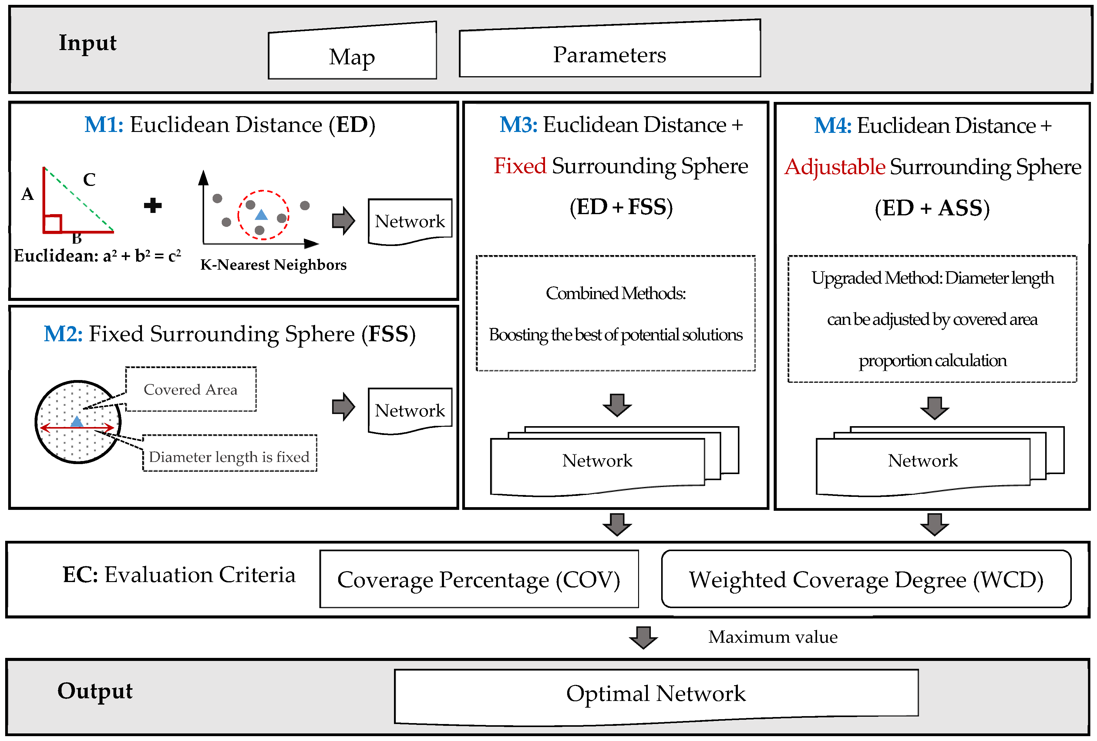
In this study, finding optimal stations’ main target goal is achieving the maximum spatial coverage while still preserving appropriate overlapping areas. The maximum spatial coverage designed can be realized through the optimal placement of the stations in the city. Moreover, maintaining a relevant overlapped area can enhance effectiveness for more reliable and accurate data collection. Accordingly, in this section, we proposed finding the stations based on the Euclidean Distance and the k-nearest neighbor’s algorithm (k-NN). The proposed methods framework consists of four main methods and two evaluation criteria, as shown in Figure 2.
In the proposed framework, our input consists of a map and parameters. The map of the study area is divided into a square of continue grid. A centroid of each square grid is a point that consists of latitude-longitude coordinates. For simple understanding throughout this paper, we use the term “location” (Li), i = 1 … N to represent the centroid of a grid. The parameters consisted of (i) a grid index at the center of the map, (ii) a specified number of stations, and (iii) the diameter length of the surrounding sphere of each station as described in Section 6.1. Next, we give stations in area A, which consist of η stations. The value S = {Sj, …, Sη} is a list of stations. Each station Sj, j = 1 … η is at a location in our study area. All of the input will use to calculate by our proposed methods.
M1: Euclidean Distance (ED) and M2: Fixed Surrounding Sphere are the initial method for finding the next stations. The M3 method is a combination of previous methods. The M4 is an upgraded version of M3. Our evaluation criteria, coverage percentage (COV), and weighted coverage degree (WCD) are used to evaluate the results from the methods then return the optimal network. The comprehensive methods are described in the following sections.
4.1. Euclidean Distance (ED)
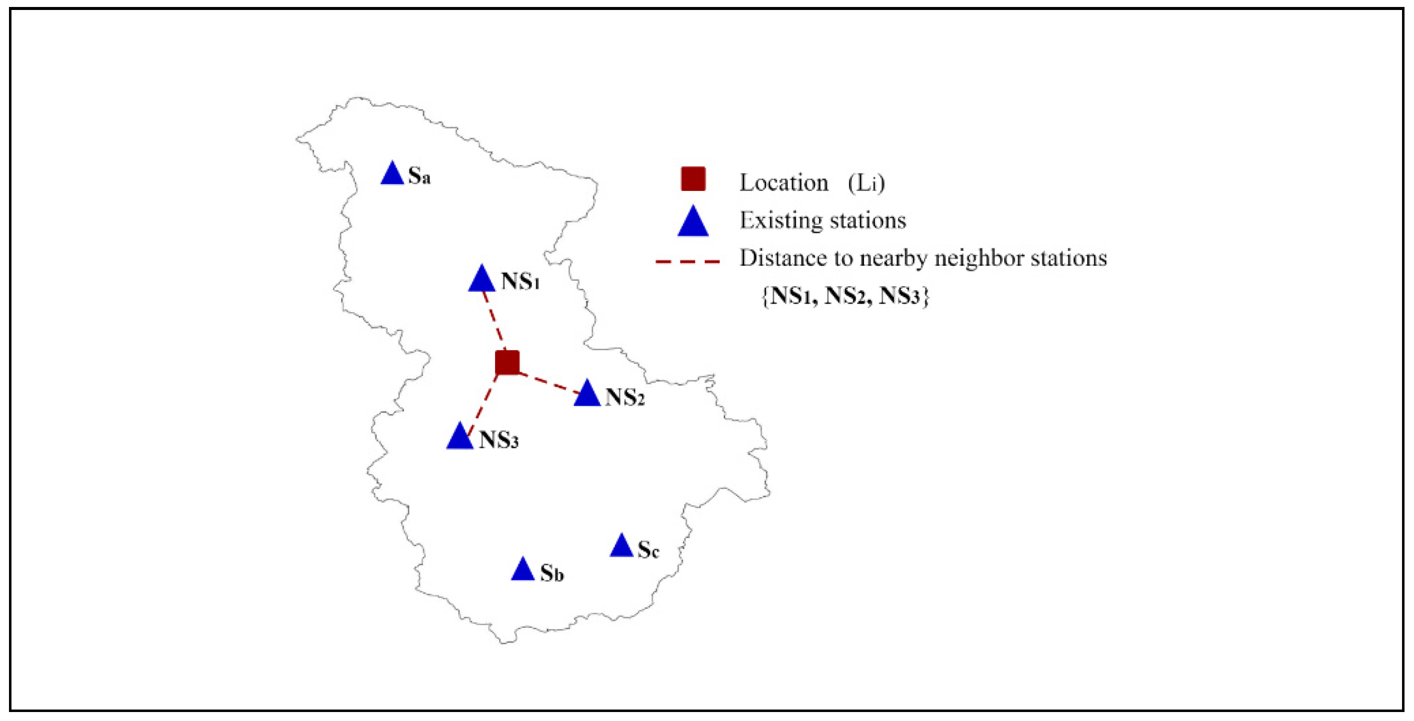
In this study, we apply the Euclidean Distance function to calculate distance from location (Li) to three nearest neighbor stations {NS1, NS2, NS3}, as illustrated in Figure 3. We use k-NN (k = 3) because the nearby stations can exchange data reliability with existing stations. Let NS1, NS2, and NS3 be members of the set of nearest neighboring stations of Li, where Li is a position to calculate EDi. We calculate the Euclidean Distance (EDi) at any Li as:
EDi denotes Euclidean Distance at Li, where i is an index of the location, and each parenthesized value is the distance from Li to NS1, NS2, and NS3, respectively. If k < 3, then we adapt the equation by using only existing stations. For example, if k = 2, then is equal to zero. Thus, EDi is calculated using only and .
In order to calculate and find the next station, the following definitions are used. Let S denote a list of stations in a network and let Lt be a candidate station to be evaluated for the possibility of it being the next station. Thus, the current station network is S + Lt. Here, we calculate EDi according to Equation (1). Subsequently, we sum EDi values as:
TEDLt denotes the total of EDi, where Lt is a candidate for the next station, and N is the number of locations. The candidate with the lowest TEDLt will be defined as the additional station.
4.2. Fixed Surrounding Sphere (FSS)
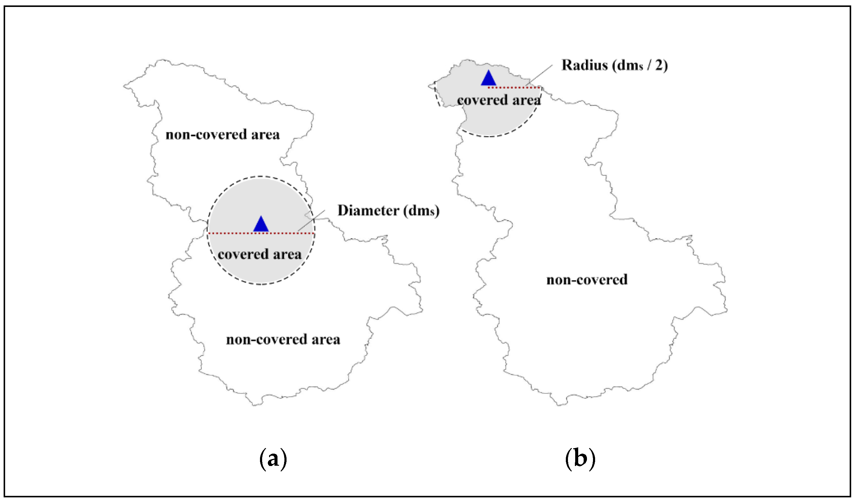
The fixed surrounding sphere (FSS) method was inspired by the original sphere of influence (SOI) [12]. We applied such an idea for determining the area surrounding each station without using pollution concentration data. The constant value is identified to a diameter length of FSS with reference to city air quality monitoring network designing in Seoul city [2]. In Seoul’s existing air monitoring network, the 25 stations are located approximately 5 km away from each other. They are not located close to the road, high emission concentration sources, or high-density population areas. On the other hand, these stations are distributed throughout the city. Consequently, we predefined a fixed diameter (dms) of FSS to divide the covered and non-covered areas under stations. As shown in Figure 4, the triangle symbols represent stations. The surrounding covered area of the stations is illustrated as a circle shape in Figure 4a and a pie shape in Figure 4b by determining a diameter length. The areas outside represent the non-covered areas. The shapes depend on the position of stations on the map. However, such areas are defined as covered areas, although the shapes of the areas are different.
The procedure to classify the covered and non-covered areas under a station are described in this subsection. Let station Sj be a location of station and the diameter of Sj be equal to . The location (Li) is covered (monitored) by a station Sj when the distance from Li to Sj is less than and also such Li will be members of all covered areas for Asj. Equation (3) represents the probability p(Li,Sj) that a location is covered by station Sj.
i is the index of location from 0 to N − 1, where N represents the number of locations in area A, and j provides an index of stations in S.
The Algorithm 1 Fixed Surrounding Sphere (FSS) can be described as follows:
| Algorithm 1. Fixed Surrounding Sphere (FSS) |
 |
4.3. Euclidean Distance + Fixed Surrounding Sphere (ED + FSS)
This method combines the concepts Euclidean Distance (ED) and Fixed Surrounding Sphere (FSS). However, the difference between this method and the previous one is the location of the first station. For ED and FSS, the first stations are set at the center of the map, while for ED + FSS, all map locations are tried as a first station. The output of this method is a multi-list of stations in which the first stations are different. Consequently, further evaluation criteria have been introduced to evaluate the best network with a maximum of spatial coverage.
We divide ED + FSS into two processes: (i) finding the next stations and (ii) evaluating a maximum coverage percentage while still preserving an appropriate overlapped area for the network. The first process, finding the next stations, is described with Algorithm 2 Euclidean Distance + Fixed Surrounding Sphere (ED + FSS) as follows:
| Algorithm 2. Euclidean Distance + Fixed Surrounding Sphere (ED + FSS) |
 |
After we obtain a multi-list of stations, the next process is to evaluate the maximum coverage percentages of all Sx. The ED + FSS will use two criteria, Coverage Percentage (COV) and Weighted Coverage Degree (WCD), for selecting the best network. The descriptions of COV and WCD criteria are outlined in Section 5.
4.4. Euclidean Distance + Adjustable Surrounding Sphere (ED + ASS)
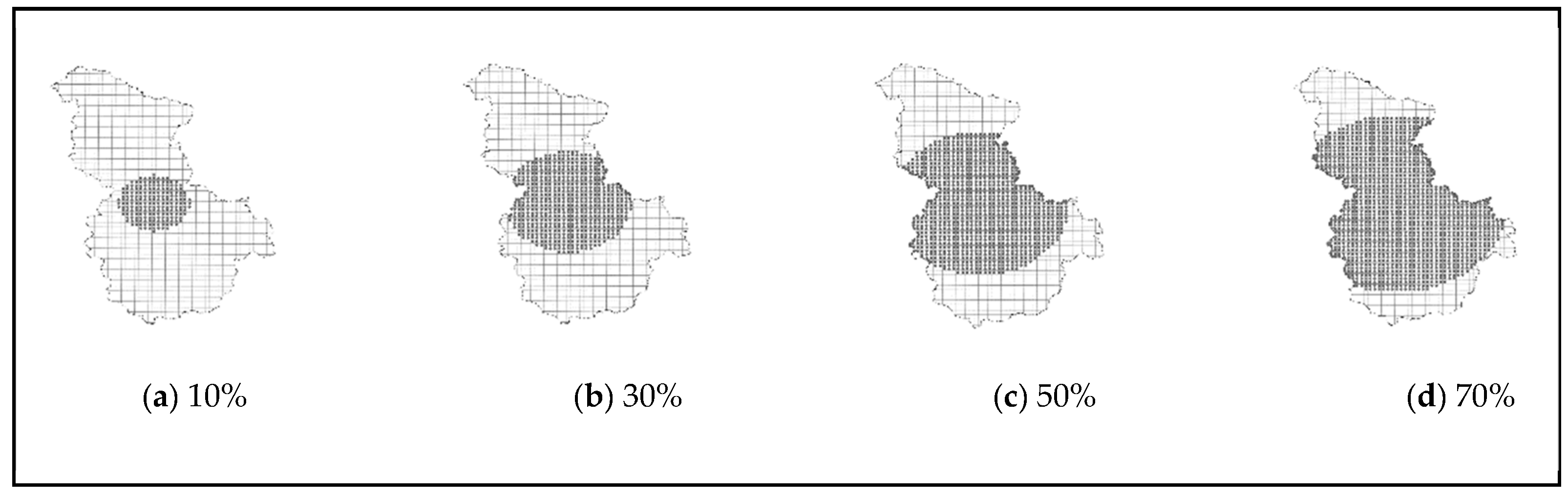
This method is an upgrade from ED + FSS. We change from using a fixed diameter to an adjustable diameter, which depends on a station’s covered area proportion. Our proposed method considers economic benefits based on deployment costs and station location with the highest spatial coverage for a specified number of economically feasible stations. The covered area proportion can be adjusted as needed. For example, if the environmental authority has a budget limit for establishing monitoring stations, an arbitrary ratio can be predefined as 50% or 70%. On the other hand, if they require high spatial resolution monitoring or an unlimited budget, the ratio can be predefined as 10% or 30%.
As a warmup to ED + ASS, we select a station at the center of the map (Scenter) for calculating the length of the diameter. Next, we calculate EDi from all locations (Li) on map to the Scenter with Equation (1). We pass all the EDi values into a list. Subsequently, we sort the obtained list in ascending order, which means that locations closer to the station with lower EDi values will be at the beginning of the list. The cut off position corresponds to an arbitrary ratio, as mentioned above. We calculate the cut off position value with Equation (4).
ratio is predefined covered area proportion of the station, length (list) is equal N where N represents the total number of locations in area.
In the sorted list, we access the index of the list at the cut off position and get the value of that EDi value. The value of EDi is multiplied by two and defined as a diameter length of the ED + ASS method. Once, we have obtained the diameter length, and then we can continue the procedure of establishing the station network and evaluating the global maximum coverage of the station network in the same way as we did with ED + FSS.
5. Evaluation Criteria
In ED + FSS and ED + ASS, there is a multi-list of station networks with different first locations that must be processed to evaluate the maximum coverage percentage. Consequently, in order to find the best station network, the evaluation criteria are designed and described next.
5.1. Coverage Percentage (COV)
The covered area of stations (AS) can be determined using Equation (3). Given the list of stations S located in a study area, we can assess the k-coverage when a location is covered by at least k different stations. The parameter k is called Coverage Degree. It means at least k stations cover each location in the study area. There are previous studies of wireless network coverage that have discussed the required k value of a network. Such studies explain a proper value of k that depends on the application. For example, an application requires k = 1 in a monitoring environment in which fault tolerance is not important. Meanwhile, k > 1 should be used when stronger monitoring is required, such as in an industrial or dangerous chemical region. Furthermore, in cases requiring fault tolerance, k ≥ 3 is required. Therefore, it is clear that the station networks with higher k-coverage are more reliable [32,33].
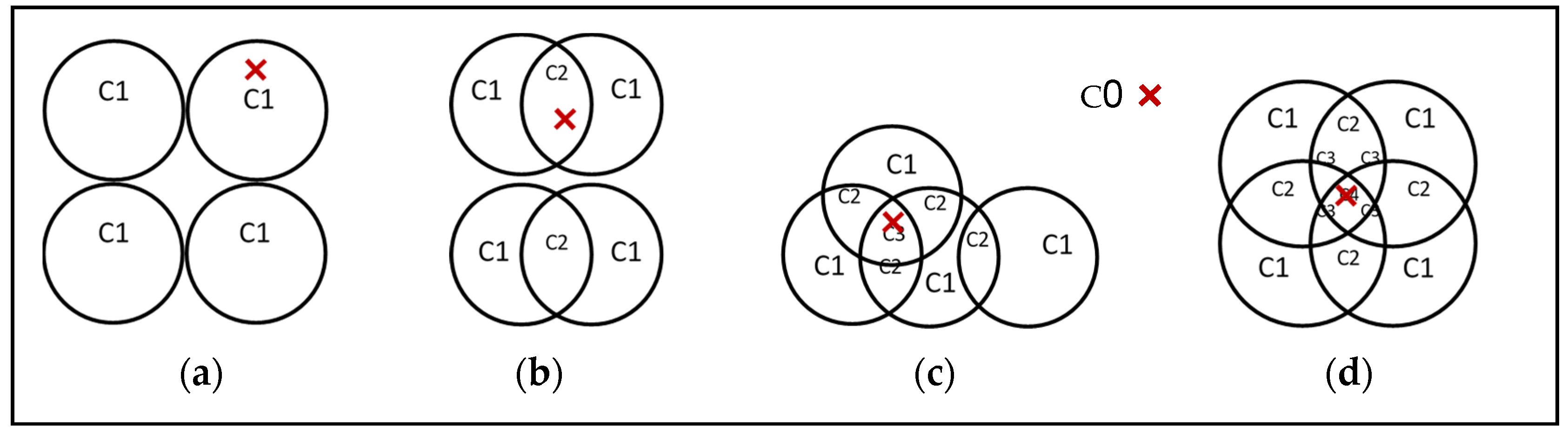
Suppose that there are four stations. The circle shapes represent covered areas of a station and × symbols represent Li for coverage degree assessment. If × symbols are within the covered areas of one station, then we define such Li as a C1. If × symbol lies within the covered areas of two, three, and four stations, then it is denoted by C2, C3, and C4 as shown in Figure 5a–d, respectively. The area outside the circle is defined as a C0, which means it is a non-covered area.
We calculate the coverage percentage using the count Li in each of the coverage degrees. The coverage percentage (COV) is used to evaluate results in our proposed methods and can be calculated with Equation (5).
Ci denotes the summation of Li in coverage degree, i is k-coverage number, k indicates a number of stations in the network, and N is total number of locations in study area A.
5.2. Weighted Coverage Degree (WCD)
Weighted coverage degree (WCD) is an additional criterion. It is used whenever COV cannot give a unique answer to the best network. The WCD corresponds to number of stations and k-coverage. For example, if the study area has four stations, here the k-coverage k = 4 (coverage degree: C0, C1, C2, C3, C4) and the weight has five values of coverage degree. We calculate the weight value by employing the Divide and Conquer concept. The ∑Wi is a value equal to one. The Wk is calculated from ∑Wi divided by two. The next weight value at Wk-i will decrease from the previous by half, which means Wk-i = Wk divided by two. The weight calculation is done continuously until the last weight at W0 is set equal to W1. Table 1 is an example of weight value generation when the coverage degree is equal to 4. The WCD can be calculated by coverage degree weighting with Equation (6).
Wi is a weight value and ∑Wi = 1, i ϵ {0, 1, 2, …, k}, k indicates a number of stations in the network, and the weights are associated to Coverage Degree (Ci).
6. Results and Discussion
This section explains the parameters used in the experiment and compares each method’s pros and cons. In scenario 1, setting up a network by considering four cases as following, (i) spatial coverage, (ii) performance of coverage percentage versus the number of the stations added incrementally, (iii) coverage percentage versus a specified number of stations, and (iv) flexibility to apply our methods to different cities. In scenario 2, finding an additional station to improve the current network is evaluated.
6.1. Experimental Parameter Settings
The parameter settings are shown in Table 2. The area size (A) is the number of locations in study areas. The centers of the maps are located at indices 1056, 3516, and 218 for Sejong, Bangkok, and Bonn. The specified number of stations is equal to the existing stations in the cities. The diameter length of the M3: ED + FSS is a fixed value of ten kilometers and the M4: ED + ASS is predetermined. We consider the proportion of covered area from reasonable based on the number of existing stations, as shown in Figure 6. Finally, we determined that 30% is a proper value for our experiment.
6.2. Assessment of Scenario 1: Setting Up a Network
6.2.1. Spatial Coverage
Table 3 shows M1: ED, M2: FSS and compares them with the existing stations in Sejong city. In Table 3, triangle symbols depict existing stations, and circles represent the spatial coverage. Let us consider a result in M1: ED, where we defined the first station at the center and used four stations as input parameters. The output from M1: ED is shown in Table 3 (b). Three stations are located near each other, but one station is located far away from its neighbors. We found significant inefficient spatial coverage in that case because almost all covered areas overlap. The COV of M1: ED is 57%, which is a 16% decrease in the current value, and WCD shows a value of 12.58, which increased 48% when compared with the current value. Next, consider the result in M2: FSS; we used the input parameters as same as M1: ED except adding a fixed diameter of ten kilometers to be used in the calculation. The result shows that most stations are located apart from the first station at the center, as shown in Table 3 (c). As a result, M2: FSS achieves the best coverage percentage up to 91% and an increase of 34% compared to the current value. On the other hand, the WCD value shows 7.44, which decreased by 13%.
The M1: ED shows large overlapping areas which make a strengthened area with neighboring stations. The area of overlap can make data more reliable in case of data verification between neighboring stations and also produce a network which is fault tolerant. We denominate such overlap areas as confidence areas because they can enhance data reliability. However, this method shows spatial coverage weaknesses. In contrast, M2: FSS shows achieving good spatial coverage which can cover an area up to 91% in the case of four stations in Sejong city. For the spatial coverage assessment, it is possible to conclude that M2: FSS is better than M1: ED.
6.2.2. Performance of Coverage Percentage Versus the Number of Stations Added Incrementally
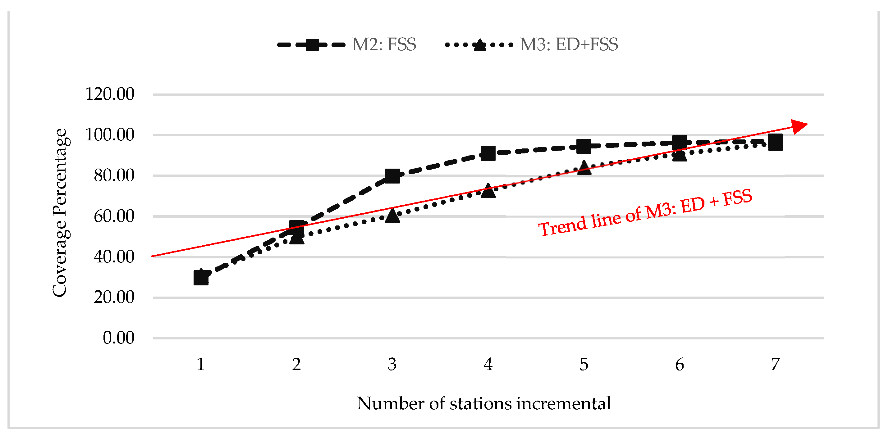
Our previous result when establishing four stations using M2: FSS shows a high coverage percentage of about 91%, which is better than M1: ED. In this case, we compared the performance of M2: FSS and M3: ED + FSS in terms of coverage percentage versus the number of stations added incrementally. The specified number of stations is seven. In Figure 7, the plot graph shows a comparison coverage percentage (COV) as the number of stations increases. The dashed line with square symbols indicates M2: FSS that shows coverage percentage increasing sharply and degrading from stations numbered 4 to 7. In contrast, the dotted line with triangle symbols indicates M3: ED + FSS and offers a relatively stable increasing trend from stations numbered 1 to 7. We conclude that M3: ED + FSS shows a coverage increasing trend better than that of M2: FSS.
Next, we investigated the additional stations of M2: FSS. As shown in Table 4 (a), light color of triangle symbols indicated the three additional stations which are located close to the border.
Although the M2: FSS achieves excellent spatial coverage (98%) nonetheless, the additional stations cause loss of area coverage, which shows the transparent area inside circles. On the other hand, all seven stations from the M3: ED + FSS method are located inside the city. These stations provide both sufficient spatial coverage (94%) and right overlapping area, as clearly shown in Table 4 (b). According to the result, we can assert a performance of M3: ED + FSS in achieving spatial coverage without loss of area coverage while still preserving the overlapped areas. The nearby stations can enhance strength to neighboring stations, which makes the network more robust and its data more reliable.
6.2.3. Coverage Percentage Versus a Specified Number of Stations
In this experimental case, we compared the performance of M3: ED + FSS and M4: ED + ASS concerning coverage percentage versus a specified number of stations. The location of station results from two methods is shown in Table 5. This part of our experiment aims to consider the flexibility of finding stations when we predefine the number of stations.
We will evaluate the coverage percentage and distribution of the stations in the study area. The results based on M3: ED + FSS show that the stations in similar aligned positions seem like a straight line in all four cases. On the other hand, results for M4: ED + ASS show a better balance of stations. The stations are readjusted whenever the number of stations changes. Furthermore, in four cases of a specified number of stations, the M4: ED + ASS has a higher coverage percentage and is better than M3: ED + FSS. Clearly, M4: ED + ASS is better than M3: ED + FSS to better cover the percentage and balance of stations.
6.2.4. Flexibility to Apply Our Methods for Different Cities
The M4: ED + ASS shows good spatial coverage and balance of stations based on a specified number of stations. For this section, we compared our method’s capability to apply to different sizes of cities and evaluated balancing and distribution of the stations in cities. We used M3: ED + FSS and M4: ED + ASS in Bangkok, Sejong, and Bonn. The cities in that list are in descending order by size.
Table 6 (bkk-1), (sj-1), and (bo-1) shows the existing stations and current coverage percentages. There are twelve stations in Bangkok, four stations in Sejong, and one station in Bonn. The result of M3: ED + FSS in Table 6 (bkk-2) shows an imbalance of stations. On the other hand, the stations from M4: ED + ASS in Table 6 (bkk-3) are evenly distributed over the city. One benefit of balancing locations and overlapping areas is that the network can better support the future urban expansion and provide better air pollution monitoring. Although in Table 6, (sj-3) and (bo-3) cannot clearly show the balancing of stations when compared with Table 6 (sj-2) and (bo-2), the COV values of M4: ED + ASS are higher than M3: ED + FSS and show significantly increased rates of 56%, 22%, and 37%, in Bangkok, Sejong, and Bonn, respectively. These results allow us to conclude that our M4: ED + ASS is more flexible than M3: ED + FSS for designing new station networks in any city size.
6.3. Assessment of Scenario 2: Finding Additional Stations to Improve the Current Network
For this section, we applied M4: ED + ASS to add one station into the network. Then, we evaluated the results with our proposed criteria: COV and WCD. In Table 7, triangle symbols indicate the existing stations, and star symbol indicates the additional station. The additional stations show the performance of our proposed method and evaluation criteria. They can improve coverage percentages by 39%, 34%, and 130% in Bangkok, Sejong, and Bonn.
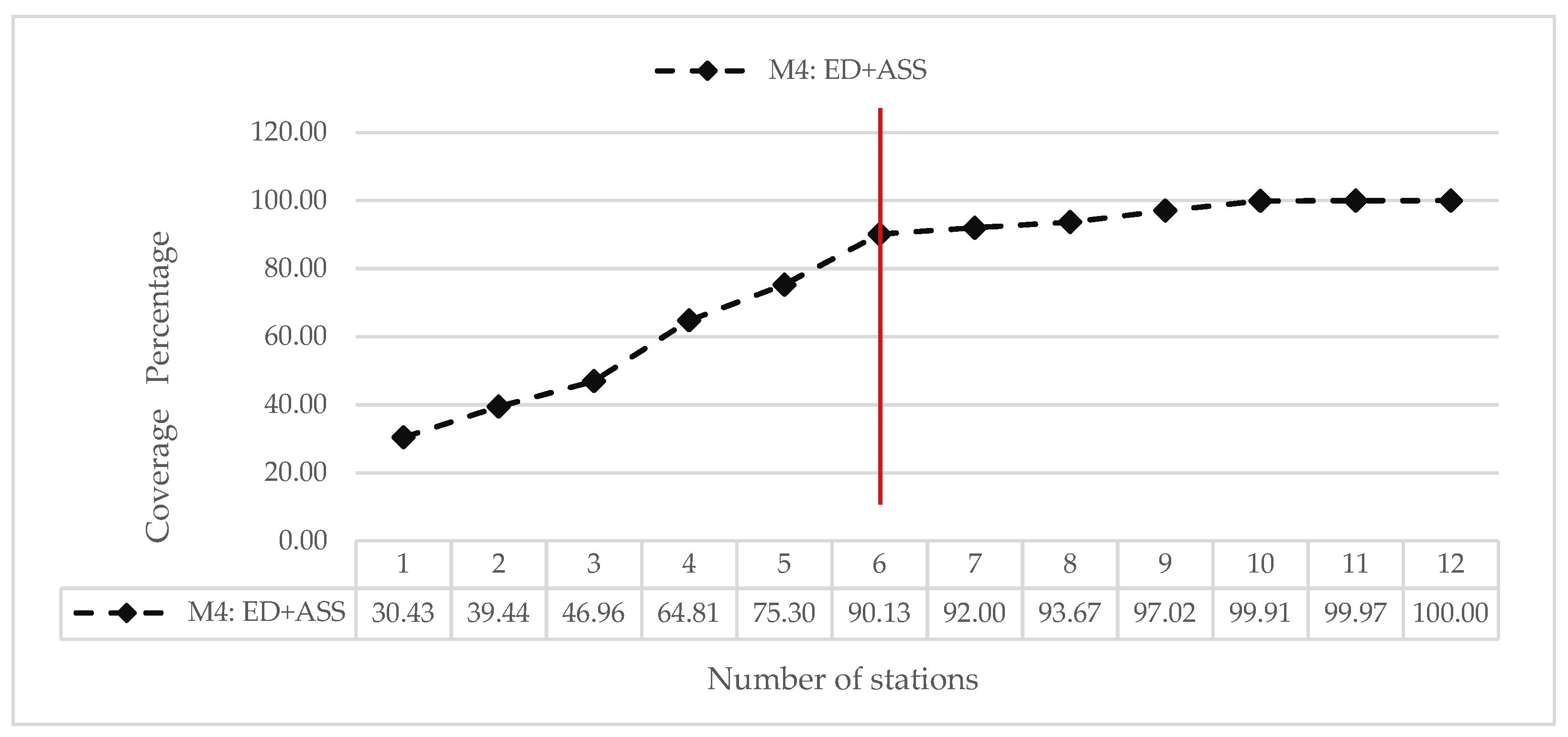
One of the key limitations of our study is the appropriate ratio of spatial coverage satisfaction versus confidence area. As shown in Figure 8, the dashed line plot graph compares coverage percentage and the number of stations. The 6th stations show the most coverage percentage of 90%. Increasing the number of stations from 7 up to 12 does not significantly increase coverage. Thus in future work, a change of strategy is needed after achieving the spatial coverage to increase the overlapped regions.
7. Conclusions
Increasing spatial coverage of AQMN gives effective environmental management. Especially in setting up a network in cities that lack historical pollution data, adding stations in cities with an existing network that face urbanization can make it challenging to design adequate spatial coverage and effective AQMN. Our experimental results proved the ability of the proposed method to provide maximum spatial coverage based on a given number of stations. The results showed that ED + ASS achieved effectiveness both in enhance spatial coverage and proper confidence area. In setting up a network in the cities, such a method suggested a balance of station locations and achieved maximum spatial coverage. The stations are neither located close to the border, nor are they close together. However, they are evenly distributed over the city. These results indicated that if the city planner considers economic benefits and the investment costs for constructing a network, the proposed method can give an excellent. In adding stations in cities, the results showed an optimal for the next station and enhanced the spatial coverage. Our proposed method showed effectiveness for expanding the existing networks as well as setting up AQMN.
In future work, we will consider the ratio of spatial coverage satisfaction versus confidence area as we mentioned in our experiment. We will modify our methods by changing strategies after achieving the spatial coverage to increase the overlapped regions of confidence areas. Moreover, we will integrate the historical pollution information, the city characteristics data, and land-use to find stations for better air pollution monitoring.
Author Contributions
Formal analysis, A.O.; methodology, A.O., H.J.; software, A.O.; validation, H.J., K.C.; investigation, A.O., H.J., writing–original draft preparation, A.O.; writing–review & editing, A.O., H.J., K.C.; supervision, H.J., K.C. All authors have read and agreed to the published version of the manuscript.
Funding
This research received no external funding.
Conflicts of Interest
The authors declare no conflict of interest.
References
- Thailand State of Pollution Report 2019, Pollution Control Department Ministry of Natural Resources and Environment. Available online: https://www.pcd.go.th/publication/8013/ (accessed on 15 August 2020).
- Seoul Solution, Air Pollution Monitoring Network. Available online: https://www.seoulsolution.kr/sites/default/files/policy/환경_2_p23_Air Pollution Monitoring Network.pdf (accessed on 3 August 2020).
- EPA: United States Environmental Protection Agency. Ambient Monitoring Guidelines for Prevention of Significant Deterioration (PSD). USA; 1987. Available online: https://www.epa.gov/nsr/ambient-monitoring-guidelines-prevention-significant-deterioration (accessed on 1 August 2020).
- National Environment Protection, Review of Air Quality Monitoring Network Design. Australian; 2019. Available online: https://www.environment.nsw.gov.au/reszearch-and-publications/publications-search/review-of-air-quality-monitoring-network-design (accessed on 1 August 2020).
- Gulia, S.; Nagendra, S.S.; Khare, M.; Khanna, I. Urban air quality management—A review. Atmos. Pollut. Res. 2015, 6, 286–304. [Google Scholar] [CrossRef] [Green Version]
- Wu, H.; Reis, S.; Lin, C.; Heal, M.R. Effect of monitoring network design on land use regression models for estimating residential NO2 concentration. Atmos. Environ. 2017, 149, 24–33. [Google Scholar] [CrossRef] [Green Version]
- Piersanti, A.; Ciancarella, L.; Cremona, G.; Righini, G.; Vitali, L. Application of a land cover indicator to characterize spatial representativeness of air quality monitoring stations over Italy. Air Pollut. Model. Appl. XXIV 2016, 625–628. [Google Scholar] [CrossRef]
- Min, K.D.; Kwon, H.J.; Kim, K.; Kim, S.Y. Air pollution monitoring design for epidemiological application in a densely populated city. Int. J. Environ. Res. Public Health 2017, 14, 686. [Google Scholar] [CrossRef] [PubMed] [Green Version]
- Pigliautile, I.; Marseglia, G.; Pisello, A.L. Investigation of CO2 variation and mapping through wearable sensing techniques for measuring pedestrians’ exposure in urban areas. Sustainability 2020, 12, 3936. [Google Scholar] [CrossRef]
- Marseglia, G.; Medaglia, C.M.; Ortega, F.A.; Mesa, J.A. Optimal alignments for designing urban transport systems: Application to Seville. Sustainability 2019, 11, 5058. [Google Scholar] [CrossRef] [Green Version]
- Baldauf, R.W.; Wiener, R.W.; Heist, D.K. Methodology for siting ambient air monitors at the neighborhood scale. J. Air Waste Manag. Assoc. 2002, 52, 1433–1442. [Google Scholar] [CrossRef] [Green Version]
- Mofarrah, A.; Husain, T. A holistic approach for optimal design of air quality monitoring network expansion in an urban area. Atmos. Environ. 2010, 44, 432–440. [Google Scholar] [CrossRef]
- Mofarrah, A.; Husain, T.; Alharbi, B.H. Design of urban air quality monitoring network: Fuzzy based multi-criteria decision making approach. Air Qual. Monit. Assess. Manag. 2011, 11, 25–39. [Google Scholar]
- Liu, M.K.; Avrin, J.; Pollack, R.I.; Behar, J.V.; McElroy, J.L. Methodology for designing air quality monitoring networks: I. Theoretical aspects. Environ. Monit. Assess. 1986, 6, 1–11. [Google Scholar] [CrossRef]
- Lin, B.; Zhu, J. Changes in urban air quality during urbanization in China. J. Clean. Prod. 2018, 188, 312–321. [Google Scholar] [CrossRef]
- Vadrevu, K.; Ohara, T.; Justice, C. Land cover, land use changes and air pollution in Asia: A synthesis. Environ. Res. Lett. 2017, 12, 120201. [Google Scholar] [CrossRef] [Green Version]
- Choung, Y.J.; Kim, J.M. Study of the Relationship between Urban Expansion and PM10 Concentration Using Multi-Temporal Spatial Datasets and the Machine Learning Technique: Case Study for Daegu, South Korea. Appl. Sci. 2019, 9, 1098. [Google Scholar] [CrossRef] [Green Version]
- Marseglia, G.; Vasquez-Pena, B.F.; Medaglia, C.M.; Chacartegui, R. Alternative fuels for combined cycle power plants: An analysis of options for a location in India. Sustainability 2020, 12, 3330. [Google Scholar] [CrossRef] [Green Version]
- Health Effects Institute, Outdoor Air Pollution and Health in the Developing Countries of Asia: A Comprehensive Review. Available online: https://www.healtheffects.org/publication/outdoor-air-pollution-and-health-developing-countries-asia-comprehensive-review (accessed on 10 October 2020).
- Zheng, J.; Feng, X.; Liu, P.; Zhong, L.; Lai, S. Site location optimization of regional air quality monitoring network in China: Methodology and case study. J. Environ. Monit. 2011, 13, 3185–3195. [Google Scholar] [CrossRef]
- Henriquez, A.; Osses, A.; Gallardo, L.; Resquin, M.D. Analysis and optimal design of air quality monitoring networks using a variational approach. Tellus B Chem. Phys. Meteorol. 2015, 67, 25385. [Google Scholar] [CrossRef] [Green Version]
- Benis, K.Z.; Fatehifar, E. Optimal design of air quality monitoring network around an oil refinery plant: A holistic approach. Int. J. Environ. Sci. Technol. 2015, 12, 1331–1342. [Google Scholar] [CrossRef] [Green Version]
- Kazemi-Beydokhti, M.; Abbaspour, R.A.; Kheradmandi, M.; Bozorgi-Amiri, A. Determination of the physical domain for air quality monitoring stations using the ANP-OWA method in GIS. Environ. Monit. Assess. 2019, 191, 299. [Google Scholar] [CrossRef]
- Li, T.; Zhou, X.C.; Ikhumhen, H.O.; Difei, A. Research on the optimization of air quality monitoring station layout based on spatial grid statistical analysis method. Environ. Technol. 2018, 39, 1271–1283. [Google Scholar] [CrossRef]
- Alsahli, M.M.; Al-Harbi, M. Allocating optimum sites for air quality monitoring stations using GIS suitability analysis. Urban Clim. 2018, 24, 875–886. [Google Scholar] [CrossRef]
- Yoo, E.C.; Park, O.H. Optimization of air quality monitoring networks in Busan using a GIS-based decision support system. J. Korean Soc. Atmos. Environ. 2007, 23, 526–538. [Google Scholar] [CrossRef]
- Shareef, M.M.; Husain, T.; Alharbi, B. Optimization of air quality monitoring network using GIS based interpolation techniques. J. Environ. Prot. 2016, 7, 895–911. [Google Scholar] [CrossRef] [Green Version]
- Liu, S.; Wei, Q.; Failler, P.; Lan, H. Fine particulate air pollution, public service, and under-five mortality: A cross-country empirical study. Healthcare 2020, 8, 271. [Google Scholar] [CrossRef] [PubMed]
- IQAir, 2019 World Air Quality Report Region & City PM2.5 Ranking. Available online: https://www.iqair.com/world-most-polluted-cities/world-air-quality-report-2019-en.pdf (accessed on 30 October 2020).
- Awe, Y.; Hagler, G.; Kleiman, G.; Klopp, J.; Pinder, R.; Terry, S. Filling the Gaps: Improving Measurement of Ambient air Quality in Low and Middle Income Countries; World Bank: Washington, DC, USA, 2017; Available online: http://pubdocs.worldbank.org/en/425951511369561703/Filling-the-Gaps-White-Paper-Discussion-Draft-November-2017.pdf (accessed on 30 October 2020).
- Desa, U.N. Transforming Our World: The 2030 Agenda for Sustainable Development. Available online: https://sdgs.un.org/2030agenda (accessed on 12 January 2021).
- Patra, R.R.; Patra, P.K. Analysis of k-coverage in wireless sensor networks. Int. J. Adv. Comput. Sci. Appl. 2011, 2, 91–96. [Google Scholar]
- Huang, C.F.; Tseng, Y.C. The coverage problem in a wireless sensor network. Mob. Netw. Appl. 2005, 10, 519–528. [Google Scholar] [CrossRef]
Figure 1.
Study areas (a–c) show administrative boundaries, and triangle symbols show current stations. The map regions (d) divided into 2024 grid cells in Sejong city.
Figure 1.
Study areas (a–c) show administrative boundaries, and triangle symbols show current stations. The map regions (d) divided into 2024 grid cells in Sejong city.

Figure 2.
The framework of proposed methods.

Figure 3.
The location of Li and its nearest neighbor stations NS1, NS2, and NS3.

Figure 4.
The (a) circle and (b) pie shapes indicate the covered areas by stations at the different positions on the map by determining a diameter length.
Figure 4.
The (a) circle and (b) pie shapes indicate the covered areas by stations at the different positions on the map by determining a diameter length.

Figure 5.
The example of coverage degree, (a–d) indicate the covered areas by one, two, three, and four stations.
Figure 5.
The example of coverage degree, (a–d) indicate the covered areas by one, two, three, and four stations.

Figure 6.
Depicts the proportion of covered area in 10%, 30%, 50%, and 70% (a–d), respectively.

Figure 7.
Plot of historical coverage percentage versus number of stations in Sejong.

Figure 8.
Plot of coverage percentage versus number of stations in Bangkok.


Table 1.
Example of weight generation.
| Coverage Degree | C4 | C3 | C2 | C1 | C0 | C4 |
|---|---|---|---|---|---|---|
| Weight, ∑Wi = 1 | W4 = 0.5 | W3 = 0.25 | W2 = 0.125 | W1 = 0.0625 | W0 = 0.0625 | W4 = 0.5 |
Table 2.
Experiment Parameter Setting.
| Parameters | Sejong | Bangkok | Bonn |
|---|---|---|---|
| Area size (A) | 2024 | 7010 | 653 |
| Index of the center of the map | 1056 | 3516 | 218 |
| Number of stations | 4 | 12 | 1 |
| Diameter length of FSS (dms) | 10 km. | 10 km. | 10 km. |
| Diameter 1 length of ASS (dms) | 14.2 km. | 25.4 km. | 8.6 km. |
1 Diameter calculation is based on proportion with a covered area of 30% for the cities.
Table 3.
The existing stations and the results of stations, coverage percentage, and weighted coverage degree of two methods: M1: ED and M2: FSS.
Table 3.
The existing stations and the results of stations, coverage percentage, and weighted coverage degree of two methods: M1: ED and M2: FSS.
| Current | M1: ED | M2: FSS | ||||
|---|---|---|---|---|---|---|
| Map of Sejong city and Stations |  (a) |  (b) |  (c) | |||
| 1. Coverage Degree & Weight | C0: 655 C1: 774 C2: 527 C3: 67 C4: 1 | W0: 0.0625 W1: 0.0625 W2: 0.125 W3: 0.25 W4: 0.5 | C0: 877 C1: 526 C2: 44 C3: 508 C4: 69 | W0: 0.0625 W1: 0.0625 W2: 0.125 W3: 0.25 W4: 0.5 | C0: 183 C1: 1513 C2: 299 C3: 29 C4: 0 | W0: 0.0625 W1: 0.0625 W2: 0.125 W3: 0.25 W4: 0.5 |
| 2. Coverage Percentage (COV) | 68% | 57% (−16%) | 91% (+34%) | |||
| 3. Weighted Coverage Degree (WCD) value | 8.52 | 12.58 (+48%) | 7.44 (−13%) | |||
Table 4.
The results of stations, coverage percentages, and weighted coverage degrees of two methods: M2: FSS and M3: ED + FSS.
Table 4.
The results of stations, coverage percentages, and weighted coverage degrees of two methods: M2: FSS and M3: ED + FSS.
| M2: FSS | M3: ED + FSS | |||
| Map of Sejong city and Stations |  (a) |  (b) | ||
| 1. Coverage Degree & Weighted | C0: 49 C1: 767 C2: 856 C3: 290 C4: 62 C5: 0 C6: 0 C7: 0 | W1: 0.0078125 W1: 0.0078125 W2: 0.015625 W3: 0.03125 W4: 0.0625 W5: 0.125 W6: 0.25 W7: 0.5 | C0: 121 C1: 520 C2: 757 C3: 584 C4: 42 C5: 0 C6: 0 C7: 0 | W1: 0.0078125 W1: 0.0078125 W2: 0.015625 W3: 0.03125 W4: 0.0625 W5: 0.125 W6: 0.25 W7: 0.5 |
| 2. Coverage Percentage (COV) | 98% | 94% | ||
| 3. Weighted Coverage Degree (WCD) value | 1.61 | 1.86 | ||
Table 5.
Location of stations within the cities and coverage percentage.
| 4 Stations | 5 Stations | 6 Stations | 7 Stations | |
|---|---|---|---|---|
| M3: ED + FSS |  COV: 76% |  COV: 87% |  COV: 91% |  COV: 94% |
| M4: ED + ASS |  COV: 83% |  COV: 93% |  COV: 97% |  COV: 99% |
Table 6.
Locations of stations within the cities and coverage percentages: (bkk-1), (sj-1), (bo-1) depict current stations, (bkk-2), (sj-2), (bo-2) depict station networks using M3: ED + FSS, and (bkk-3), (sj-3), (bo-3) depict station networks improved using M4: ED + ASS, in Bangkok, Sejong, and Bonn, respectively.
| Country/Methods | Bangkok, Thailand (1568.7 km2) | Sejong, Korea (465.23 km2) | Bonn, Germany (141.06 km2) |
|---|---|---|---|
| Current |  (bkk-1) COV: 64% |  (sj-1) COV: 68% |  (bo-1) COV: 27% |
| M3: ED + FSS |  (bkk-2) COV: 99% (+55%) |  (sj-2) COV: 76% (+12%) |  (bo-2) COV: 33% (+22%) |
| M4: ED + ASS |  (bkk-3) COV: 100% (+56%) |  (sj-3) COV: 83% (+22%) |  (bo-3) COV: 37% (+37%) |
Table 7.
Location of an additional station and resulting coverage percentages in Bangkok, Sejong, and Bonn.
Table 7.
Location of an additional station and resulting coverage percentages in Bangkok, Sejong, and Bonn.
| Bangkok, Thailand | Sejong, Korea | Bonn, Germany |
|---|---|---|
 COV: 89% (+39%) |  COV: 91% (+34%) |  COV: 62% (+130%) |
Publisher’s Note: MDPI stays neutral with regard to jurisdictional claims in published maps and institutional affiliations. |
© 2021 by the authors. Licensee MDPI, Basel, Switzerland. This article is an open access article distributed under the terms and conditions of the Creative Commons Attribution (CC BY) license (http://creativecommons.org/licenses/by/4.0/).
Share and Cite
MDPI and ACS Style
Onuean, A.; Jung, H.; Chinnasarn, K. Finding Optimal Stations Using Euclidean Distance and Adjustable Surrounding Sphere. Appl. Sci. 2021, 11, 848. https://doi.org/10.3390/app11020848
AMA Style
Onuean A, Jung H, Chinnasarn K. Finding Optimal Stations Using Euclidean Distance and Adjustable Surrounding Sphere. Applied Sciences. 2021; 11(2):848. https://doi.org/10.3390/app11020848
Chicago/Turabian StyleOnuean, Athita, Hanmin Jung, and Krisana Chinnasarn. 2021. "Finding Optimal Stations Using Euclidean Distance and Adjustable Surrounding Sphere" Applied Sciences 11, no. 2: 848. https://doi.org/10.3390/app11020848
Note that from the first issue of 2016, this journal uses article numbers instead of page numbers. See further details here.