An Adaptive Optimization Method Based on Learning Rate Schedule for Neural Networks

Abstract

Artificial intelligence (AI) is achieved by optimizing the cost function constructed from learning data. Changing the parameters in the cost function is an AI learning process (or AI learning for convenience). If AI learning is well performed, then the value of the cost function is the global minimum. In order to obtain the well-learned AI learning, the parameter should be no change in the value of the cost function at the global minimum. One useful optimization method is the momentum method; however, the momentum method has difficulty stopping the parameter when the value of the cost function satisfies the global minimum (non-stop problem). The proposed method is based on the momentum method. In order to solve the non-stop problem of the momentum method, we use the value of the cost function to our method. Therefore, as the learning method processes, the mechanism in our method reduces the amount of change in the parameter by the effect of the value of the cost function. We verified the method through proof of convergence and numerical experiments with existing methods to ensure that the learning works well.

1. Introduction

Artificial intelligence (AI) is completed by defining the cost function constructed through an artificial neural network (ANN) from given learning data, and by determining the parameters that minimize this cost function. In other words, AI learning is the cost function optimization process. Therefore, AI learning has two problems to solve—the definition and the optimization of the cost function. The first problem, the definition of the cost function, is the more data and the more complicated the structure of the ANN. For this reason, the cost function is increased the complexity [1,2,3,4,5]. The complexity here means that the number of local minimums of the cost function increases. The local minimum of the cost function is the part that makes the first order derivative of the cost function zero. Therefore, if AI learning is continued as a learning method based on the first order derivative of the cost function, the learning is not performed at this local minimum. Therefore, as the local minimum part of the cost function increases, AI learning does not proceed smoothly. In order to take advantage of more applications and AI, the amount of data increases and the structure of the ANN becomes more complicated. AI learning should be conducted using the cost function containing many local minimums. That is, the second problem arises in which the optimization problem is solved for the cost function containing many local minimums [6,7,8,9,10].

The main purpose of this paper is to solve the second problem, that is, we want to complete AI learning based on the first derivative of the cost function in a cost function that contains many local minimums. In order to complete AI learning, we introduce the method of adding the first order derivative of the cost function to the cost function so that the learning is carried out using the global minimum. Therefore, the mathematical Lagrangian method is used [11,12]. Additionally, the most powerful of the existing methods based on the first derivative of the cost function is the momentum method [13,14]. The momentum method consists of adding the first derivative of the cost function by multiplying it by a certain ratio, that is, the learning of the parameters is accomplished by the added values of the first derivative [15,16,17,18,19,20]. Therefore, even if the first derivative of the cost function is zero at a local minimum, learning can continue based on the previously added first derivative of the cost function. The problem with this method is that, even when we are well educated (situations where we need to stop learning), learning continues based on the previously added first derivative of the cost function. As learning continues, learning does not stop, and when learning is completed, optimal learning may not have been achieved. In order to solve this problem, methods using the change of the learning rate (step size) and adding an adaptive property to the momentum method have been developed [21,22,23,24]. This paper is based on the momentum method and adds an adaptive property, which constitutes a step size change with the degree of the cost function. It maintains the power of the momentum method, adds adaptive properties to it to make a certain percentage of learning, and finally constructs a step size according to the amount of the cost function, making it as close as possible to the minimum value of the cost function. More specific ideas and methods are discussed in detail in the text. This paper also proves that the parameters defined in our method converge. In this paper, we use the usual notations found in mathematics for convenience.

This paper is organized as follows—Section 2 introduces the cost function and the momentum method; Section 3 explains our proposed method; Section 4 confirms our claim through numerical experiments; and the conclusions are presented in Section 5.

2. The Optimization Problem and the Momentum Method

From the learning data, we defined the cost function. The learning data were divided into the input data $\left\{x_j\right\}$ and the output data $\left\{y_j\right\}$. From the input data $\left\{x_j\right\}$ and using an ANN, we defined $y_{h,j}=y_h(\mathbf{w},x_j)$, where $\mathbf{w}$ is a learning parameter. AI learning was completed with the definition of the learning parameter w that satisfies $y_{h,j}=y_j$.

2.1. The Optimization Problem

In order to satisfy $y_{h,j}=y_j$, we constructed the cost function as:

$$\begin{array}{c}\hfill C\left(\mathbf{w}\right)=\frac{1}{l}\sum _{j=1}^l{\left(y_j-y_{h,j}\right)}^2,\end{array}$$

(1)

where l is an integer (number of learning data), and we solved the following the optimization problem:

$$\begin{array}{c}\hfill argmi{n}_{\mathbf{w}}\left\{C\left(\mathbf{w}\right)\right\}.\end{array}$$

(2)

To solve the optimization problem (2), gradient-based methods are generally used [1,3]. Gradient-based methods are used to find parameter $\mathbf{w}$, such that the gradient of the cost function is zero. However, the cost function $C\left(\mathbf{w}\right)$ is not convex in general. If the cost function $C\left(\mathbf{w}\right)$ is not convex, the idea of zeroing the gradient may not work well. Therefore, in order to increase the efficiency of learning, we applied the Lagrange multiplier method to define $F\left(\mathbf{w}\right)$ as follows, and to find the parameter $\mathbf{w}$ that makes $F\left(\mathbf{w}\right)$ zero.

$$\begin{array}{c}\hfill F\left(\mathbf{w}\right):=\frac{\partial C\left(\mathbf{w}\right)}{\partial \mathbf{w}}+\mu C\left(\mathbf{w}\right),\end{array}$$

(3)

where $\mu$ is a small constant. In order to obtain $\mathbf{w}$ that satisfies Equation (3) by resulting in zero, we used an iterative parameter change rule:

$$\begin{array}{c}\hfill {\mathbf{w}}_{i+1}={\mathbf{w}}_i-\lambda F\left({\mathbf{w}}_i\right),\end{array}$$

(4)

where $\lambda$ is a constant and is called the learning rate. Equation (4) is similar to the momentum method.

2.2. The Momentum Method

In order to solve $F\left(\mathbf{w}\right)=0$, the momentum method is:

$$\begin{array}{c}\hfill {\mathbf{w}}_{i+1}={\mathbf{w}}_i-{\mathbf{m}}_i,\end{array}$$

where $m_i={\sum }_{k=1}^i{\beta }_1^{k-1}F\left({\mathbf{w}}^{i-k+1}\right)$ and ${\beta }_1<1$. The momentum method multiplies the ratio of ${\beta }_1$, and thus has the problem that $\mathbf{w}$ changes continuously even when $F\left(\mathbf{w}\right)$ becomes zero. Therefore, the momentum method needs a way to stop learning.

3. Our Proposed Method

Our method is based on the momentum method that stops the learning at the moment when it meets the global minimum value of the cost function, which is the moment when learning is well executed. By changing the learning rate, the following is obtained:

$$\begin{array}{ccc}\hfill {\mathbf{w}}_{i+1}& =& {\mathbf{w}}_i-{\eta }_i{\mathbf{m}}_i,\hfill \end{array}$$

(5)

where:

$$\begin{array}{c}\hfill {\eta }_i={\eta }_0\frac{C\left({\mathbf{w}}_i\right)}{\sqrt{{\mathbf{v}}_i+ϵ}},\end{array}$$

(6)

where ${\eta }_0$ is a constant, and:

$$\begin{array}{c}\hfill {\mathbf{v}}_i=\sum _{k=1}^i{\beta }_2^{k-1}{\left(F\left({\mathbf{w}}_{i-k+1}\right)\right)}^2.\end{array}$$

In particular, $ϵ$ is a constant introduced to prevent division by zero.

Lemma 1.

The relationship between ${\mathbf{m}}_i$ and ${\mathbf{v}}_i$ is:

$$\begin{array}{c}\hfill {\left({\mathbf{m}}_i\right)}^2\le \left(\frac{1-{\left(\frac{{\beta }_1^2}{{\beta }_2}\right)}^i}{1-\left(\frac{{\beta }_1^2}{{\beta }_2}\right)}\right){\mathbf{v}}_i.\end{array}$$

Proof. 

The proof can be found in [19]. □

Using the relationship between ${\mathbf{m}}_i$ and ${\mathbf{v}}_i$, from Equation (5), we have:

$$\begin{array}{ccc}\hfill ⟹& & \left|{\mathbf{w}}_{i+1}-{\mathbf{w}}_i\right|\le {\eta }_{0}C\left({\mathbf{w}}_i\right){\left(\frac{1-{\left(\frac{{\beta }_1^2}{{\beta }_2}\right)}^i}{1-\left(\frac{{\beta }_1^2}{{\beta }_2}\right)}\right)}^{1/2}.\hfill \end{array}$$

(7)

Here, since $ϵ$ is to prevent division by zero, it can be considered as zero in the calculation. Therefore, the sequence $\left\{{\mathbf{w}}_i\right\}$ also converges when the sequence $\left\{{\eta }_i\right\}$ converges to zero.

Theorem 1.

We need to find the parameter that minimizes the cost function C. The limit value of our constructed sequence $\left\{{\mathbf{w}}_i\right\}$ is a sequence that gives the value of the cost function C as zero. The closer the cost function C is to zero, the closer the relationship between $y_{h,j}$ and $y_j$ (the value of $y_{h,j}$ made through the ANN approaches the output value $y_j$).

Proof. 

After a sufficiently large number $\tau$, a sufficiently small value ${\eta }_i$, and using the Taylor’s theorem, the following calculation is performed:

$$\begin{array}{c}\hfill C\left({\mathbf{w}}_{i+1}\right)=C\left({\mathbf{w}}_i\right)+\frac{\partial C}{\partial \mathbf{w}}\left({\mathbf{w}}_i\right)\left({\mathbf{w}}_{i+1}-{\mathbf{w}}_i\right)+O\left({\left({\mathbf{w}}_{i+1}-{\mathbf{w}}_i\right)}^2\right),\end{array}$$

(8)

where part of $O\left({\left({\mathbf{w}}_{i+1}-{\mathbf{w}}_i\right)}^2\right)$ represents the second order and is ignored. From Equations (5) and (8), we have:

$$\begin{array}{ccc}\hfill C\left({\mathbf{w}}_{i+1}\right)& =& C\left({\mathbf{w}}_i\right)+\frac{\partial C}{\partial \mathbf{w}}\left({\mathbf{w}}_i\right)\left({\mathbf{w}}_{i+1}-{\mathbf{w}}_i\right)\hfill \\ & =& C\left({\mathbf{w}}_i\right)-{\eta }_{0}C\left({\mathbf{w}}_i\right)\frac{\partial C}{\partial \mathbf{w}}\left({\mathbf{w}}_i\right)\left(\frac{{\mathbf{m}}_i}{{\left({\mathbf{v}}_i+ϵ\right)}^{1/2}}\right)\hfill \\ & =& C\left({\mathbf{w}}_i\right)\left(1-{\eta }_0\frac{\partial C}{\partial \mathbf{w}}\left({\mathbf{w}}_i\right)\left(\frac{{\mathbf{m}}_i}{{\left({\mathbf{v}}_i+ϵ\right)}^{1/2}}\right)\right)\hfill \\ & =& C\left({\mathbf{w}}_i\right)\left(1-{\eta }_0\left(\frac{{\left(\frac{\partial C}{\partial \mathbf{w}}\left({\mathbf{w}}_i\right)\right)}^2+\mu C\left({\mathbf{w}}_i\right)\frac{\partial C}{\partial \mathbf{w}}\left({\mathbf{w}}_i\right)+{\beta }_1\frac{\partial C}{\partial \mathbf{w}}\left({\mathbf{w}}_i\right){\mathbf{m}}_{i-1}}{{\left({\mathbf{v}}_i+ϵ\right)}^{1/2}}\right)\right).\hfill \end{array}$$

Since ${\beta }_1<1$, $ϵ\ne 0$, and adjusting ${\eta }_0$ and $\mu$:

$$\begin{array}{c}\hfill 0<{\eta }_0\left(\frac{{\left(\frac{\partial C}{\partial \mathbf{w}}\left({\mathbf{w}}_i\right)\right)}^2+\mu C\left({\mathbf{w}}_i\right)\frac{\partial C}{\partial \mathbf{w}}\left({\mathbf{w}}_i\right)+{\beta }_1\frac{\partial C}{\partial \mathbf{w}}\left({\mathbf{w}}_i\right){\mathbf{m}}_{i-1}}{{\left({\mathbf{v}}_i+ϵ\right)}^{1/2}}\right)<1\end{array}$$

Therefore, the following is obtained:

$$\begin{array}{c}\hfill C\left({\mathbf{w}}_i\right)\le {\delta }^{i-\tau }C\left({\mathbf{w}}_{\tau }\right),\end{array}$$

where:

$$\delta =supremu{m}_{i>\tau }\left\{1-{\eta }_0\left(\frac{{\left(\frac{\partial C}{\partial \mathbf{w}}\left({\mathbf{w}}_i\right)\right)}^2+\mu C\left({\mathbf{w}}_i\right)\frac{\partial C}{\partial \mathbf{w}}\left({\mathbf{w}}_i\right)+{\beta }_1\frac{\partial C}{\partial \mathbf{w}}\left({\mathbf{w}}_i\right){\mathbf{m}}_{i-1}}{{\left({\mathbf{v}}_i+ϵ\right)}^{1/2}}\right)\right\}$$

and ${lim}_{i\to \infty }C\left({\mathbf{w}}_i\right)=0$. □

In Theorem (1), it is possible that $\delta$ is less than 1. Therefore, we explain in more detail that $\delta$ is less than 1 in the following corollary.

Corollary 1.

δ defined in Theorem (1) is less than 1.

Proof. 

First of all, i is assumed to be from a number after a sufficiently large number $\tau$. Under the condition of sufficiently small values ${\eta }_i$ and $\mu$, the equation:

$${\eta }_0\left(\frac{{\left(\frac{\partial C}{\partial \mathbf{w}}\left({\mathbf{w}}_i\right)\right)}^2+\mu C\left({\mathbf{w}}_i\right)\frac{\partial C}{\partial \mathbf{w}}\left({\mathbf{w}}_i\right)+{\beta }_1\frac{\partial C}{\partial \mathbf{w}}\left({\mathbf{w}}_i\right){\mathbf{m}}_{i-1}}{{\left({\mathbf{v}}_i+ϵ\right)}^{1/2}}\right),$$

is divided into three parts and is computed as:

$$\begin{array}{c}\hfill 0<\left(\frac{{\left(\frac{\partial C}{\partial \mathbf{w}}\left({\mathbf{w}}_i\right)\right)}^2}{{\left({\mathbf{v}}_i+ϵ\right)}^{1/2}}\right)<1,\end{array}$$

(9)

$$\begin{array}{c}\hfill 0<\left|\frac{\mu C\left({\mathbf{w}}_i\right)\frac{\partial C}{\partial \mathbf{w}}\left({\mathbf{w}}_i\right)}{{\left({\mathbf{v}}_i+ϵ\right)}^{1/2}}\right|<1,\end{array}$$

(10)

and

$$\begin{array}{c}\hfill \left(\frac{{\beta }_1\frac{\partial C}{\partial \mathbf{w}}\left({\mathbf{w}}_i\right){\mathbf{m}}_{i-1}}{{\left({\mathbf{v}}_i+ϵ\right)}^{1/2}}\right).\end{array}$$

(11)

Equations (9) and (10) are obtained by easy calculation, by condition of the cost function ($C<1$), and by $\mu$. We should show that Equation (11) is less than 1. Under the assumption in this corollary and from the definition of ${\mathbf{m}}_i$, the result is $sign\left({\mathbf{m}}_i\right)=sign(\partial C\left({\mathbf{w}}_i\right)/\partial \mathbf{w})$ because ${\beta }_1<1$, and the sign does not change dramatically, since $\partial C\left(\mathbf{w}\right)/\partial \mathbf{w}$ is a continuous function. Therefore, $sign(\partial C\left({\mathbf{w}}_i\right)/\partial \mathbf{w}{\mathbf{m}}_{\mathbf{i}-\mathbf{1}})>\mathbf{0}$. From Equation (11), the following is obtained:

$$\begin{array}{ccc}\hfill {\beta }_1\frac{\partial C}{\partial \mathbf{w}}\left({\mathbf{w}}_i\right)\frac{{\mathbf{m}}_{i-1}}{{\left({\mathbf{v}}_i+ϵ\right)}^{1/2}}& =& {\beta }_1\frac{\partial C}{\partial \mathbf{w}}\left({\mathbf{w}}_i\right)\frac{{\mathbf{m}}_{i-1}}{{\left({\mathbf{v}}_{i-1}+ϵ\right)}^{1/2}}\left(\frac{{\left({\mathbf{v}}_{i-1}+ϵ\right)}^{1/2}}{{\left({\mathbf{v}}_i+ϵ\right)}^{1/2}}\right)\hfill \\ & \le & {\beta }_1\left|\frac{\partial C}{\partial \mathbf{w}}\left({\mathbf{w}}_i\right)\right|{\left(\frac{1-{\left(\frac{{\beta }_1^2}{{\beta }_2}\right)}^{i-1}}{1-\left(\frac{{\beta }_1^2}{{\beta }_2}\right)}\right)}^{1/2}\left(\frac{{\left({\mathbf{v}}_{i-1}+ϵ\right)}^{1/2}}{{\left({\mathbf{v}}_i+ϵ\right)}^{1/2}}\right)\hfill \\ & \le & {\beta }_1\left|\frac{\partial C}{\partial \mathbf{w}}\left({\mathbf{w}}_i\right)\right|{\left(\frac{1}{1-\left(\frac{{\beta }_1^2}{{\beta }_2}\right)}\right)}^{1/2}<{\beta }_1.\hfill \end{array}$$

If $sign(\partial C\left({\mathbf{w}}_i\right)/\partial \mathbf{w}{\mathbf{m}}_{\mathbf{i}-\mathbf{1}})<\mathbf{0}$, then there is a $\zeta \in [{\mathbf{w}}_i,{\mathbf{w}}_{i-1}]$ or $[{\mathbf{w}}_{i-1},{\mathbf{w}}_i]$, such that $\partial C\left(\zeta \right)/\partial \mathbf{w}\approx 0$. Therefore, $\partial C\left({\mathbf{w}}_i\right)/\partial \mathbf{w}\approx 0$. Equation (11) is a small value less than 1. By this process, we set ${\eta }_0$ constant to a small value, resulting in the following: $\delta =supremu{m}_{i>\tau }\left\{1-{\eta }_0\left(\frac{{\left(\frac{\partial C}{\partial \mathbf{w}}\left({\mathbf{w}}_i\right)\right)}^2+\mu C\left({\mathbf{w}}_i\right)\frac{\partial C}{\partial \mathbf{w}}\left({\mathbf{w}}_i\right)+{\beta }_1\frac{\partial C}{\partial \mathbf{w}}\left({\mathbf{w}}_i\right){\mathbf{m}}_{i-1}}{{\left({\mathbf{v}}_i+ϵ\right)}^{1/2}}\right)\right\}<1$. □

4. Numerical Tests

Since our method is based on the momentum method and includes the effect of said momentum method, this paper compared GD, Adam, Adagrad, and our proposed method. In Section 4.1 and Section 4.2, the performance of each method was compared by assuming a two-variable function as the cost function. This is a visualization to easily show how each method changes the parameters. In Section 4.3, we experimented with the problem of classifying the numbers from 0 to 9 written by humans. This is the most basic dataset to compare the performance of machine learning. This dataset called Modified National Institute of Standard and Technology (MNIST, see: http://yann.lecun.com/exdb/mnist/). This experiment was performed by combining the MNIST dataset and the convolution neural network (CNN) method, which is widely used for image classification. This method is a well-known method that is typically used as a method of classifying images [6].

4.1. Three-Dimensional Surface with One Local Minimum: Weber’s Function

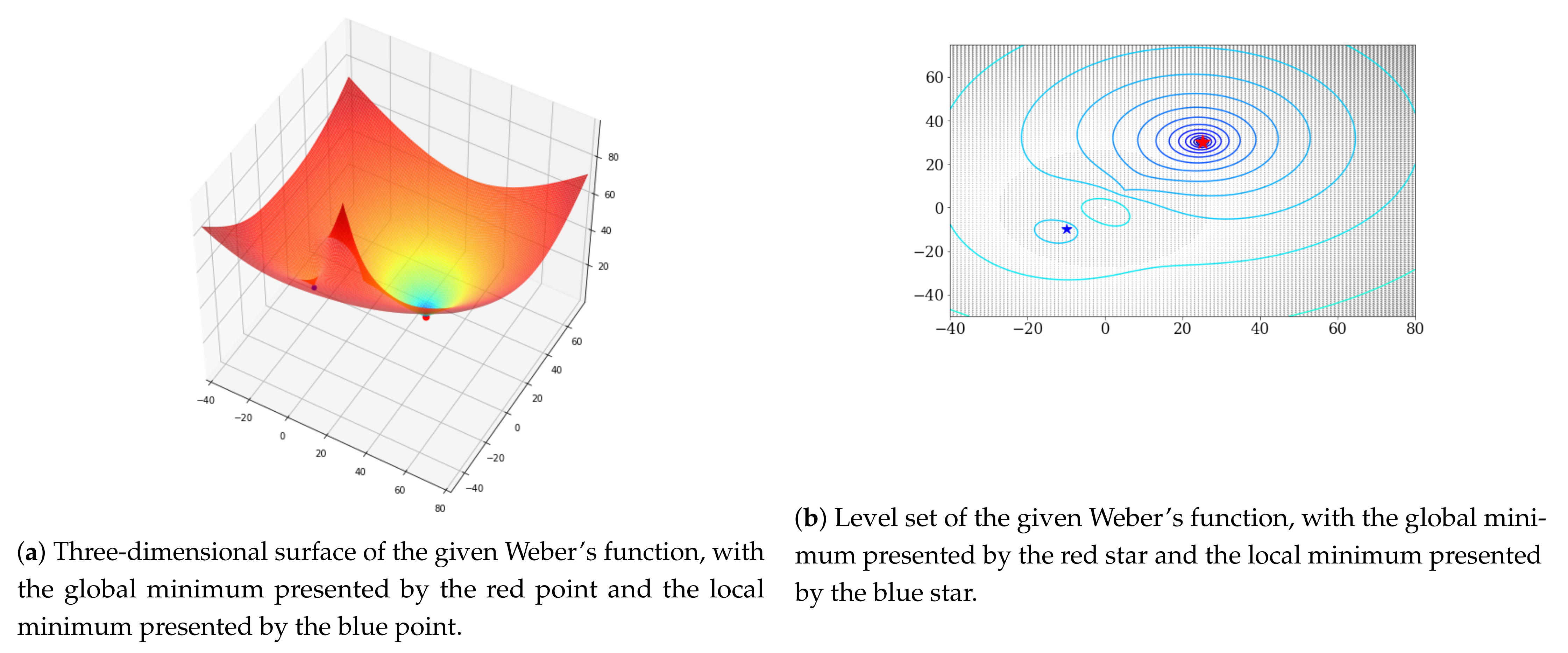
This section visualizes how each method changes parameters using the two-variable function. The two-variable function (i.e., Weber’s function) used in this experiment is generally defined as follows:

$$\begin{array}{c}\hfill C\left(\mathbf{w}\right)=\sum _{i=1}^{\kappa }{\mu }_i\sqrt{{\left({\mathbf{w}}_1-{\nu }_{i,1}\right)}^2+{\left({\mathbf{w}}_2-{\nu }_{i,2}\right)}^2},\end{array}$$

where ${\sum }_{i=1}^{\kappa }{\mu }_i>0$, $\kappa$ is an integer, and ${\mu }_i\in \mathbb{R}$. For convenience, $\nu =({\nu }_1,{\nu }_2,{\nu }_3,{\nu }_4)$ and ${\nu }_i$ is a column vector in ${\mathbb{R}}^2$. For experiments of local minimums in existing cases, we used the following hyperparameters: $\kappa =4$, $\mu =(2,-4,2,1)$, ${\nu }_1=(-10,-10)$, ${\nu }_2=(0,0)$, ${\nu }_3=(5,8)$, and ${\nu }_4=(25,30)$. This Weber’s function has a local minimum of $(-10,-10)$ and a global minimum of $(25,30)$.

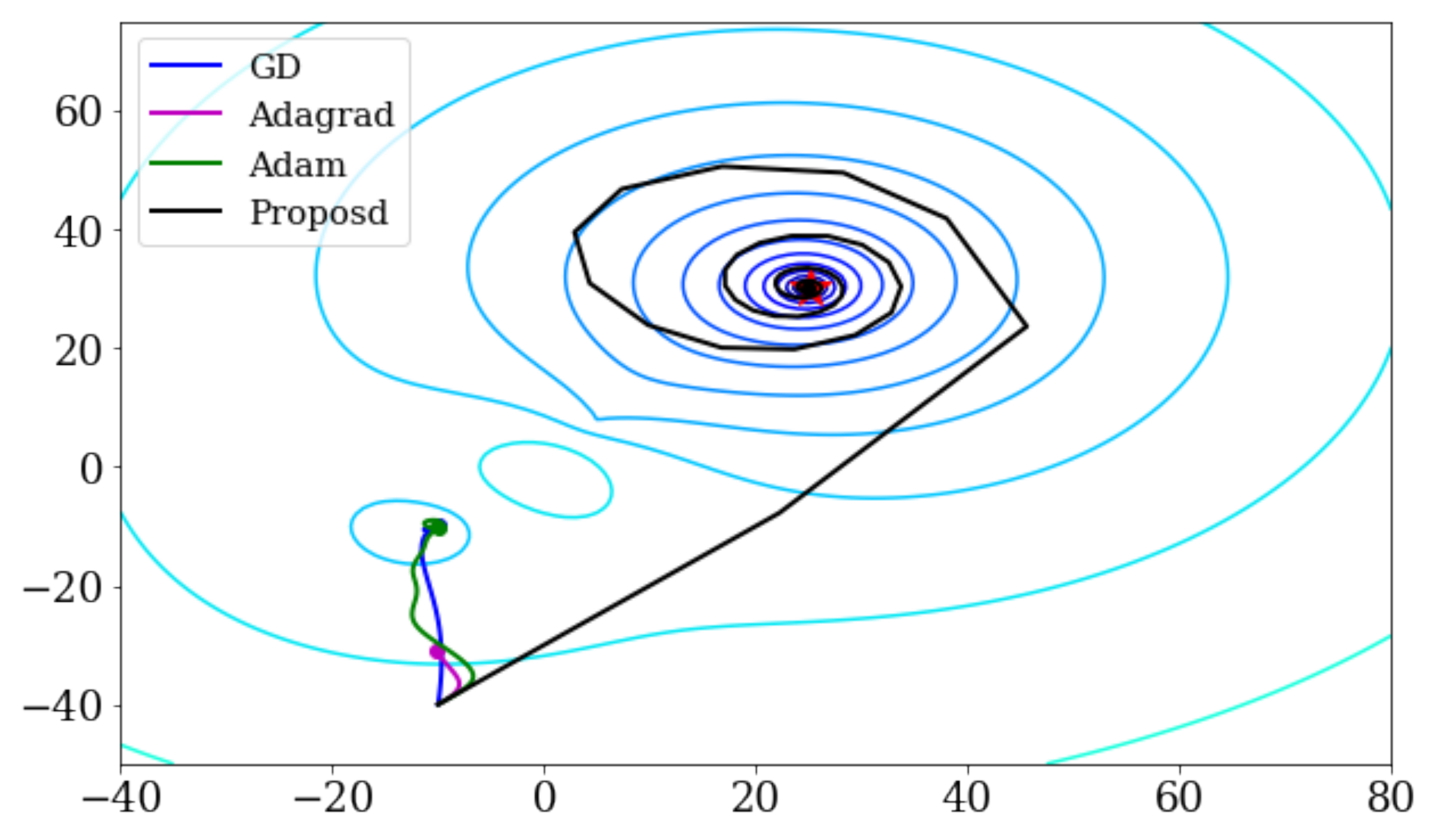
Figure 1a shows Weber’s function determined by the given $\mu$ and $\nu$. This function has a global minimum of $(25,30)$ and a local minimum of $(-10,-10)$, which are represented by the red and blue points in Figure 1a, respectively. In order to express the change of the parameters more easily, Figure 1b connects the given Weber’s function with the same function value as the contour line used on the map. In this experiment, the initial value of the parameter was set to $(-10,-40)$ and the learning rate was $5\times {10}^{-1}$, in order to check whether any of the methods has an effect of escaping the local minimum.

Figure 2 shows the change of the parameters by each method. GD, Adagrad, and Adam moved in the direction of the local minimum near the initial value and were no longer minimized; however, our proposed method avoided the local minimum to reach the global minimum.

4.2. Three-Dimensional Surface with Three Local Minimums: The Styblinski–Tang Function

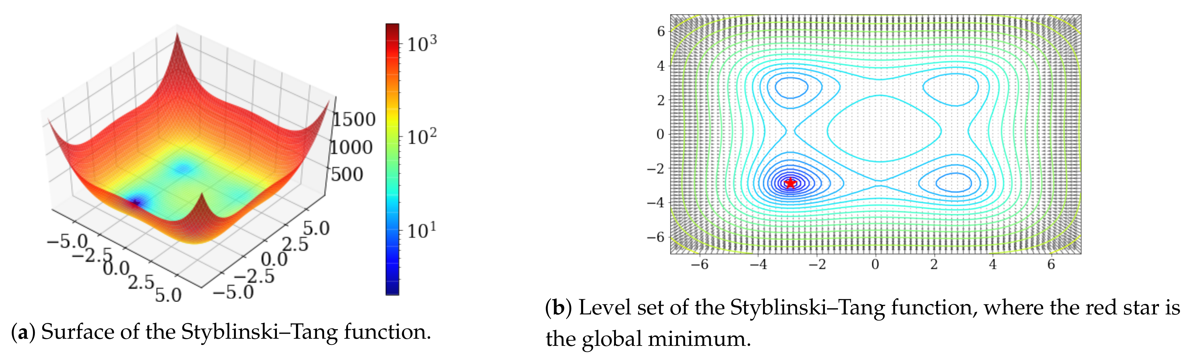
In this experiment, the performance of each method was compared using the Styblinski–Tang function with three local minimums as the cost function. The Styblinski–Tang function with three local minima is defined by:

$$\begin{array}{c}\hfill C({\mathbf{w}}_1,{\mathbf{w}}_2)=\frac{\left({\mathbf{w}}_1^4-16{\mathbf{w}}_1^2+5{\mathbf{w}}_1\right)+\left({\mathbf{w}}_2^4-16{\mathbf{w}}_2^2+5{\mathbf{w}}_2\right)}{2},\end{array}$$

and has a global minimum of $(-2.903,-2.903)$. Figure 3 is expressed in the same way as in the previous section.

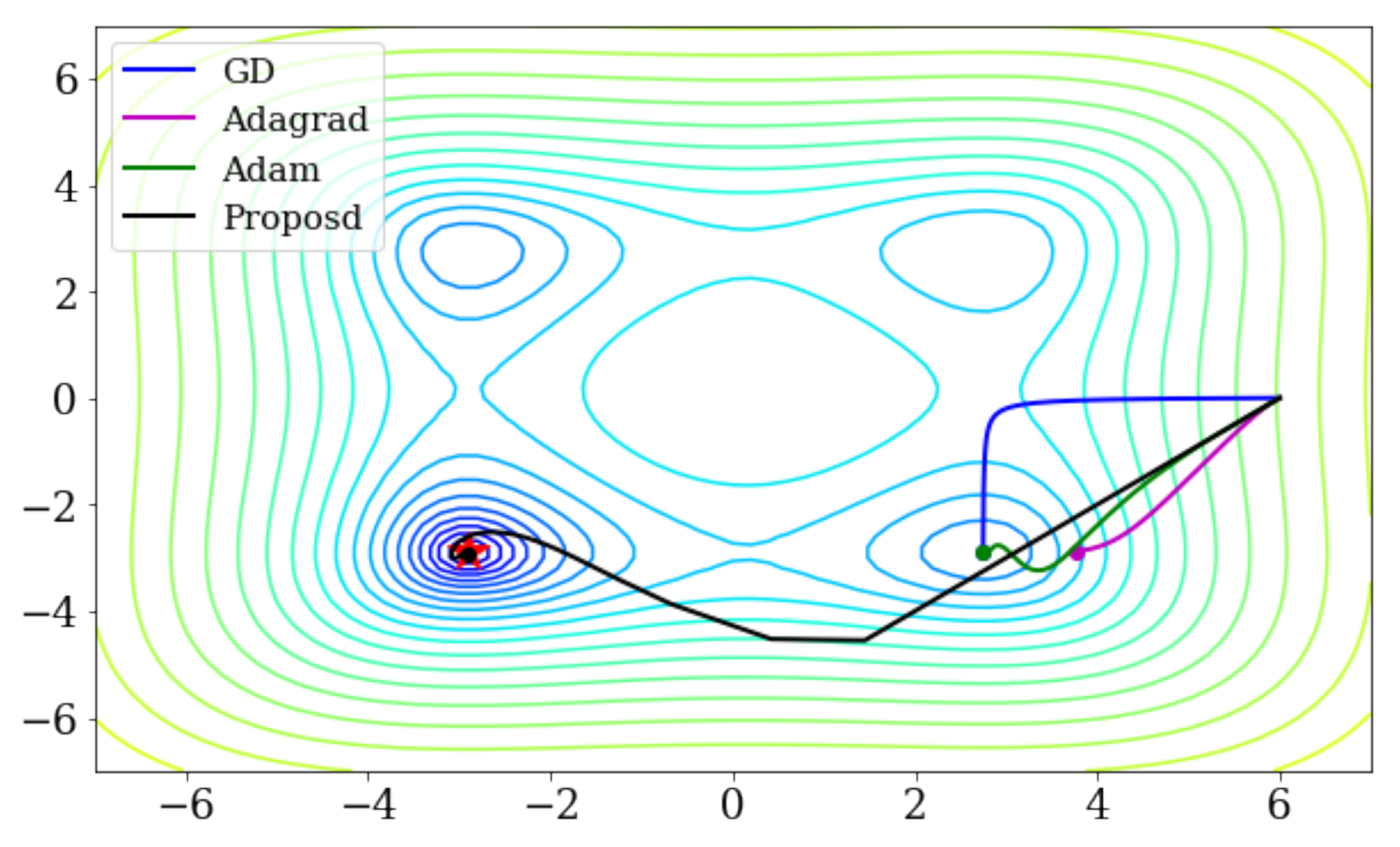
The initial value of the parameter is $(6,0)$, the learning rate is $1\times {10}^{-2}$, and learning has been conducted 300 times. Figure 4 shows the change in the parameters learned by each method. In this experiment, GD, Adagrad, and Adam also moved toward the local minimum near the initial value; however, our proposed method avoided the local minimum to reach the global minimum.

4.3. MNIST with CNN

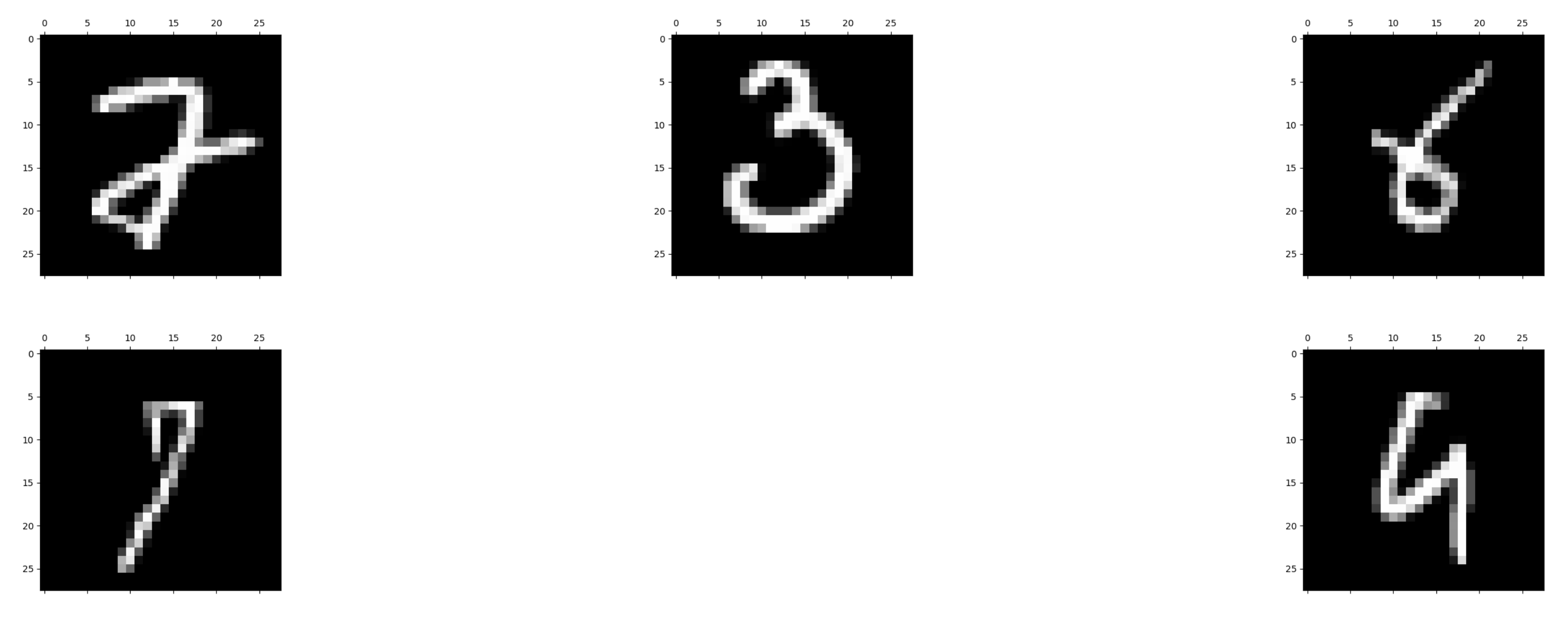
MNIST dataset are popular for machine learning and consist of a 10-class gray-scale image with a size of 28 × 28. Figure 5 shows part of the MNIST data.

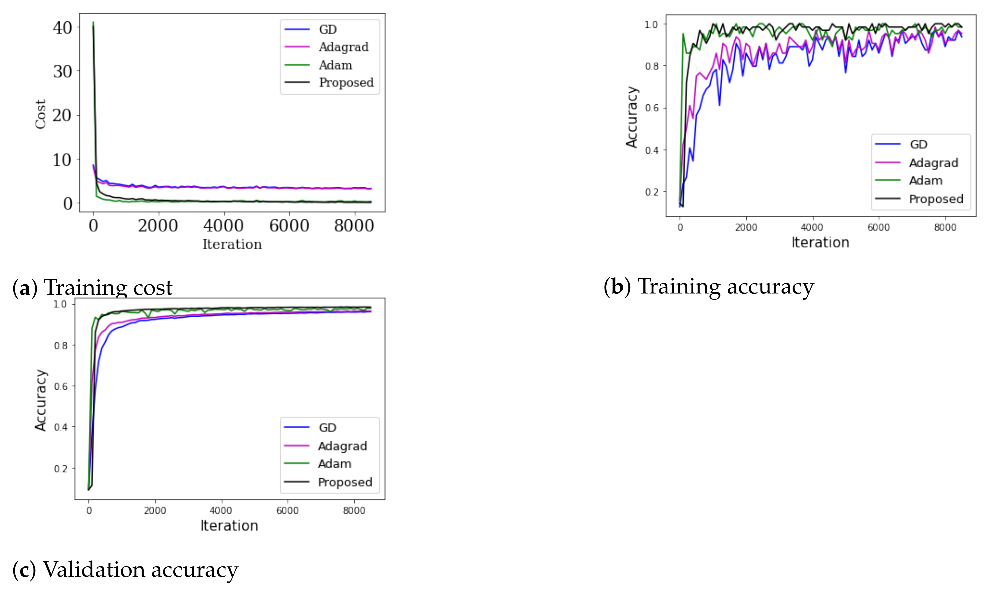
For a performance comparison of each method, a simple structured CNN consisting of two convolution layers and one hidden layer was used. For the convolution, a $5\times 5\times 32$ sized filter and $5\times 5\times 32\times 64$ sized filter were used, the batch size was set to 64, and a dropout of 50% was performed. Learning was conducted 8800 times, and the learning rate was 0.001. Figure 6 shows the results of the experiment.

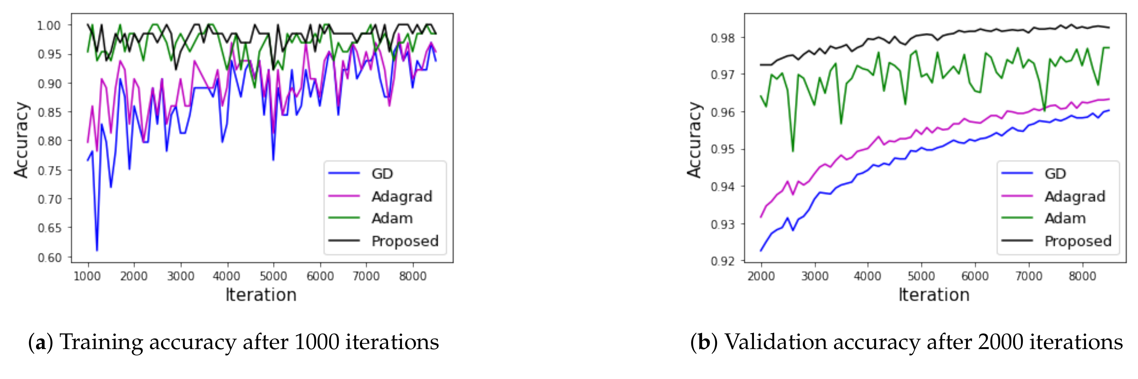
Figure 6a shows the change in cost according to the learning using each method, and shows that all of the methods minimized the cost. Figure 6b shows the accuracy using the learning data as the learning progresses, and Figure 6c shows the validation accuracy using the test data as the learning progresses to check if it is over-fitting. For a more detailed comparison, Figure 7 shows the accuracy after a certain iteration.

Figure 7a shows the training accuracy after conducting 1000 iterations, while Figure 7b shows the validation accuracy after conducting 2000 iterations. The training accuracy was high for all methods; however, Adam and our proposed method were particularly high. The order of validation accuracy from high to low is: our proposed method > Adam > Adagrad > GD.

4.4. CIFAR-10

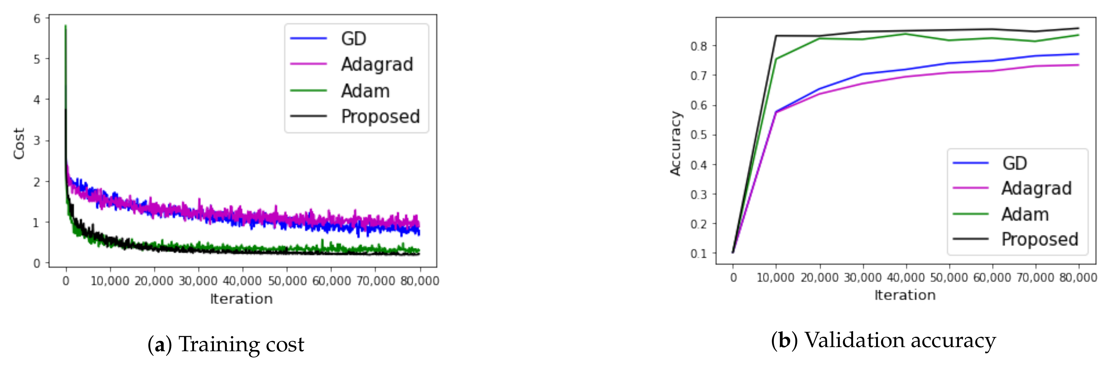
In this section, the Canadian Institute For Advanced Research-10 (CIFAR-10) dataset was trained with a residual network (RESNET) model to check the performance of each method in a more deep model. The CIFAR-10 dataset had 60,000 images. The image of the CIFAR-10 dataset used were in color (size $32\times 32$) with 10 different classes (i.e., airplanes, cars, birds, cats, deer, dogs, frogs, horses, ships, and trucks). The RESNET 44 model was used for the learning; the batch size was 128, the learning rate was 0.001, and the number of iterations was 80,000. Figure 8 shows the results of each method used in this experiment.

Figure 8a shows the training cost of each method, while Figure 8b shows the verification accuracy of each method per 10,000 steps. In Figure 8a, Adam and the proposed method had the lowest costs, and the proposed method experienced little vibration. Therefore, it seems to be a stable learning method. In Figure 8b, the proposed method achieved the best performance, followed by the Adam method.

5. Conclusions

For AI learning, we introduced a method based on the existing momentum method, using the first derivative of the cost function and the cost function at the same time. In addition, our proposed method was introduced to stop learning in an optimal situation by adjusting the learning rate in a way that responds to changes in the cost function. Our proposed method was verified not only through mathematical proofs, but also through the results of numerical experiments. It was confirmed through numerical experiments that learning through this process is superior to the existing GD, momentum, and Adam methods. In particular, through experiments, we confirmed that the stopping of learning is also important in terms of effective learning, because it results in better accuracy than other methods in terms of learning accuracy. In other words, in order for machine learning to work well, it is important to stop learning at the right moment and at the same time, as there are many changes in variables.

In the future, not only will learning stop at a useful moment in machine learning, but the problem of stopping learning will be achieved at the same time as effective learning in an ANN with a deeper structure.

References

- Bishop, C.M.; Wheeler, T. Pattern Recognition and Machine Learning; Springer: Berlin/Heidelberg, Germany, 2006. [Google Scholar]
- Rumelhart, D.E.; Hinton, G.E.; Williams, R.J. Learning representations by back-propagating errors. Nature 1986, 323, 533–536. [Google Scholar] [CrossRef]
- Goodfellow, I.; Bengio, Y.; Courville, A. Deep Learning; The MIT Press Cambridge: London, UK, 2016. [Google Scholar]
- Dean, J.; Corrado, G.; Monga, R.; Chen, K.; Devin, M.; Le, Q.; Mao, M.; Ranzato, M.; Senior, A.; Tucker, P.; et al. Large scale distributed deep networks. In Proceedings of the 25th International Conference on Neural Information Processing Systems—NIPS 2012, Lake Tahoe, NV, USA, 3–6 December 2012; pp. 1223–1231. [Google Scholar]
- Hinton, G.; Deng, L.; Yu, D.; Dahl, G.E.; Mohamed, A.; Jaitly, N.; Senior, A.; Vanhoucke, V.; Nguyen, P.; Sainath, T.N. Deep neural networks for acoustic modeling in speech recognition: The shared views of four research groups. Signal Process. Mag. 2012, 29, 82–97. [Google Scholar] [CrossRef]
- Krizhevsky, A.; Sutskever, I.; Hinton, G.E. Imagenet classification with deep convolutional neural networks. In Proceedings of the Neural Information Processing Systems—NIPS 2012, Lake Tahoe, NV, USA, 3–6 December 2012; pp. 1097–1105. [Google Scholar]
- Pascanu, R.; Bengio, Y. Revisiting natural gradient for deep networks. arXiv 2013, arXiv:1301.3584. [Google Scholar]
- Graves, A.; Mohamed, A.; Hinton, G.E. Speech recognition with deep recurrent neural networks. In Proceedings of the 2013 International Conference on Acoustics, Speech and Signal Processing—ICASSP 2013, Vancouver, BC, Canada, 26–31 May 2013; pp. 6645–6649. [Google Scholar]
- Hinton, G.E.; Srivastava, N.; Krizhevsky, A.; Sutskever, I.; Salakhutdinov, R.R. Improving neural networks by preventing co-adaptation of feature detectors. arXiv 2012, arXiv:1207.0580. [Google Scholar]
- Kochenderfer, M.; Wheeler, T. Algorithms for Optimization; The MIT Press Cambridge: London, UK, 2019. [Google Scholar]
- Kelley, C.T. Iterative methods for linear and nonlinear equations. In Frontiers in Applied Mathematics; SIAM: Philadelphia, PA, USA, 1995. [Google Scholar]
- Kelley, C.T. Iterative Methods for Optimization. In Frontiers in Applied Mathematics; SIAM: Philadelphia, PA, USA, 1999. [Google Scholar]
- Duchi, J.; Hazan, E.; Singer, Y. Adaptive subgradient methods for online learning and stochastic optimization. J. Mach. Learn. Res. 2011, 12, 2121–2159. [Google Scholar]
- Sutskever, I.; Martens, J.; Dahl, G.; Hinton, G.E. On the importance of initialization and momentum in deep learning. In Proceedings of the 30th International Conference on Machine Learning—ICML 2013, Atlanta, GA, USA, 16–21 June 2013; pp. 1139–1147. [Google Scholar]
- Tieleman, T.; Hinton, G.E. Lecture 6.5—RMSProp, COURSERA: Neural Networks for Machine Learning; Technical Report; University of Toronto: Toronto, ON, Canada, 2012. [Google Scholar]
- Zeiler, M.D. Adadelta: An adaptive learning rate method. arXiv 2012, arXiv:1212.5701. [Google Scholar]
- Kingma, D.P.; Ba, J. ADAM: A method for stochastic optimization. In Proceedings of the 3rd International Conference for Learning Representations—ICLR 2015, San Diego, CA, USA, 7–9 May 2015. [Google Scholar]
- Reddi, S.J.; Kale, S.; Kumar, S. On the Convergence of ADAM and Beyond. arXiv 2019, arXiv:1904.09237. [Google Scholar]
- Yi, D.; Ahn, J.; Ji, S. An Effective Optimization Method for Machine Learning Based on ADAM. Appl. Sci. 2020, 10, 1073. [Google Scholar] [CrossRef] [Green Version]
- Bottou, L.; Curtis, F.E.; Nocedal, J. Optimization Methods for Large-Scale Machine Learning. SIAM Rev. 2018, 60, 223–311. [Google Scholar] [CrossRef]
- Nesterov, Y. Introductory Lectures on Convex Optimization: A Basic Course; Springer: Berlin/Heidelberg, Germany, 2004. [Google Scholar]
- Bengio, Y. Practical recommendations for gradient-based training of deep architectures. arXiv 2012, arXiv:1206.5533. [Google Scholar]
- Ge, R.; Kakade, S.M.; Kidambi, R.; Netrapalli, P. The Step Decay Schedule: A Near Optimal, Geometrically Decaying Learning Rate Procedure For Least Squares. arXiv 2019, arXiv:1904.12838. [Google Scholar]
- Li, Z.; Arora, S. An Exponential Learning Rate Schedule for Deep Learning. arXiv 2019, arXiv:1910.07454. [Google Scholar]
Figure 1.
Weber’s function for the given and .
Figure 2.
Visualization of the changing parameters by each method.
Figure 3.
Styblinski–Tang function.
Figure 4.
Figure 5.
Examples of the Modified National Institute of Standard and Technology (MNIST) dataset.
Figure 6.
Results of MNIST with a convolutional neural network (CNN).
Figure 7.
Accuracy of MNIST with a CNN.
Figure 8.
Results of the Canadian Institute For Advanced Research-10 (CIFAR-10) dataset with a residual network (RESNET).
Publisher’s Note: MDPI stays neutral with regard to jurisdictional claims in published maps and institutional affiliations. |
© 2021 by the authors. Licensee MDPI, Basel, Switzerland. This article is an open access article distributed under the terms and conditions of the Creative Commons Attribution (CC BY) license (http://creativecommons.org/licenses/by/4.0/).
Share and Cite
MDPI and ACS Style
Yi, D.; Ji, S.; Park, J. An Adaptive Optimization Method Based on Learning Rate Schedule for Neural Networks. Appl. Sci. 2021, 11, 850. https://doi.org/10.3390/app11020850
AMA Style
Yi D, Ji S, Park J. An Adaptive Optimization Method Based on Learning Rate Schedule for Neural Networks. Applied Sciences. 2021; 11(2):850. https://doi.org/10.3390/app11020850
Chicago/Turabian StyleYi, Dokkyun, Sangmin Ji, and Jieun Park. 2021. "An Adaptive Optimization Method Based on Learning Rate Schedule for Neural Networks" Applied Sciences 11, no. 2: 850. https://doi.org/10.3390/app11020850
Note that from the first issue of 2016, this journal uses article numbers instead of page numbers. See further details here.