Enhancing Accuracy of Runge–Kutta-Type Collocation Methods for Solving ODEs


Faculty of Mechanical Engineering, University of Ljubljana, 1000 Ljubljana, Slovenia
*
Author to whom correspondence should be addressed.
Mathematics 2021, 9(2), 174; https://doi.org/10.3390/math9020174
Submission received: 30 December 2020
/
Revised: 11 January 2021
/
Accepted: 13 January 2021
/
Published: 16 January 2021
(This article belongs to the Special Issue Numerical Methods for Solving Differential Problems)
Abstract
:In this paper, a new class of Runge–Kutta-type collocation methods for the numerical integration of ordinary differential equations (ODEs) is presented. Its derivation is based on the integral form of the differential equation. The approach enables enhancing the accuracy of the established collocation Runge–Kutta methods while retaining the same number of stages. We demonstrate that, with the proposed approach, the Gauss–Legendre and Lobatto IIIA methods can be derived and that their accuracy can be improved for the same number of method coefficients. We expressed the methods in the form of tables similar to Butcher tableaus. The performance of the new methods is investigated on some well-known stiff, oscillatory, and nonlinear ODEs from the literature.
1. Introduction
A special type of initial value problems, treated in this work, involves highly oscillatory systems and problems known as stiff systems. In the field of numerical analysis, scientific computing, and engineering, many such problems exhibit these properties [1,2,3]. Ordinary differential equations (ODEs) describing these systems are ill-conditioned in a computational sense and challenging to solve [1]. For such problems, implicit Runge–Kutta (RK) methods are a convenient and frequent choice. The methods gained prominence after Butcher showed that the s-stage fully implicit Gaussian RK method of order 2s is A-stable for all s [4].
A subset of implicit RK methods involves collocation methods. They yield a continuous approximation which makes them suitable for problems where globally continuously differentiable functions are required [5]. Despite being known for decades, the methods are still under continuous development. Publications examine the application of the methods to new problems, the derivation of new strategies, or the development of new procedures for solving nonlinear equations [3]. Three basic types of implicit RK methods, each based on different Gauss–Legendre-type quadrature formulae, are Gauss–Legendre quadrature formulae, Gauss–Radau quadrature formulae, and Gauss–Lobatto quadrature formulae [6].
Perez-Rodriguez et al. [7] applied an implicit RK method of Radau IIA type to semi-discretized, multidimensional partial differential equations (PDEs) of advection–diffusion–reaction type. To mitigate the stiffness of these systems, a special iteration technique was applied to solve the resulting implicit relations encountered in the integration steps. Ramos and Garcia-Rubio [8] constructed a new family of implicit methods on the basis of the s-degree Chebyshev approximation using the Chebyshev–Gauss–Lobatto points. Similarly, Vigo-Aguiar and Ramos [9], in addition to constructing an A-stable iRK method, proposed an embedding technique for changing the step size using the Runge–Kutta method and a linear multistep one. Teh and Yaacob [10] recently developed several implicit RK methods, two of them being Gauss–Kronrod methods with five stages and order 8 accuracy. These are based on five-point Gauss–Kronrod quadrature formula. They also developed four implicit RK methods on the basis of Gauss–Kronrod–Radau quadrature formulae [11] and four seven-stage 10th-order implicit RK methods using seven-point Gauss–Kronrod–Lobatto quadrature formula [6]. Liu and Sun [12] studied the Lobatto III-type RK methods. They extended the existing Lobatto methods using the W-transformation and constructed general Lobatto III methods with three parameters of stages two to four. Implicit RK methods play a vital role in solving systems of differential algebraic equations (DAEs) [13]. For example, Jay [14] analyzed the application of RK methods to DAEs of index-2 in Hessenberg form and (see [15]) applied the s-stage Lobatto IIIA–Lobatto IIIB method as a partitioned RK method to integrate Hamiltonian systems with holonomic constraints. A particularly important type of implicit RK methods for stiff and DAE problems involves the Radau IIA methods, implemented in the well-known code for stiff and DAE systems, RADAU5 [16].
In this work, we present a new class of collocation methods for numerical integration of ODEs by basing the derivation on their integral form. The approach resembles the well-known Galerkin method, which is based on the so-called weak formulation of the governing differential equations; nevertheless, we could not find any references involving applying the presented idea to initial value problems and deriving collocation methods. With the approach, we present how the accuracy of RK-type collocation methods (more specifically, the Gauss–Legendre and Lobatto IIIA method) can be increased while retaining the number of method coefficients. In addition to proposing some method instances of the new class of methods, we also demonstrate how the Gauss–Legendre and Lobatto IIIA methods can also be derived with the proposed approach.
In this paper, some theoretical preliminaries are given first (Section 2), followed by a general derivation of the method (Section 3). Particular method families are then presented in Section 4 where their accuracy and linear stability are also investigated. The performance of methods is analyzed using several numerical examples in Section 5. The discussion and conclusion then follow in Section 6 and Section 7.
2. Theoretical Preliminaries
Consider the following initial value problem:
with , , for which we seek an approximate solution in the interval , with as the step size. Collocation methods utilize a polynomial, say , of degree to approximate the solution . The polynomial needs to satisfy the initial condition and the differential equation at collocation points for , with . The numerical solution of the collocation method is defined by .
The general class of RK methods is defined as follows [17]:
where a fully implicit RK method is obtained when the upper limit r in the sum defining the is equal to s. The collocation method is equivalent to the s-stage RK method, Equation (2), with the following coefficients:
where is the Lagrange polynomial [18]. The choice of coefficients and , and points defines a method instance. This work limits the arbitrary choice of points to either the roots of Legendre polynomials or a combination of Legendre polynomials of different stages. RK method subclasses based on these collocation points are Gauss–Legendre, Radau, and Lobatto [19]. The Gauss–Legendre quadrature employs a shifted Legendre polynomial of degree on the interval .
The method subclass accuracy is of order 2 and its stability function is the diagonal (,)-Padé approximation [20]. The “Radau I quadrature formula” defines as the zeros of a polynomial , yielding , while the “Radau II quadrature formula” yields on the basis of the polynomial . The “Lobatto III quadrature formula” with both and originates from the polynomial . The accuracy of the -stage Radau IA and Radau IIA methods is of order , and their stability function is the (,) subdiagonal Padé approximation. The accuracy of the Lobatto III class of method is of order , with the stability function being the diagonal (,) Padé approximation for Lobato IIIA and IIIB and (,) for Lobatto IIIC [20].
In contrast to classical collocation methods, the novel method class is derived from the integral form of Equation (1).
where is the test function, arbitrary in general. The usage of the integral approach is, for instance, widely employed in finite element formulation. Its property is a functional approximation of the observed (primary) variable which needs to satisfy the governing (partial) differential equation in an integral fashion. The approximation function, denoted as , is assumed to approximate the solution of the differential equation . The system of equations determining the approximation polynomial is constructed by substituting different test functions in Equation (5) and imposing the initial condition.
A new class of methods follows from Equation (5) by, firstly, employing different approximation polynomial functions for . Functions are defined on the basis of roots of the Legendre polynomial or its combinations (recall: , or ). The choice of then determines the quadrature rule in integrating the left-hand side of Equation (5). Secondly, different quadrature formulae are employed for the integration of the right-hand side of Equation (5). This integration can be conducted by any quadrature rule (Gauss–Legendre, Radau I, Radau II, or Lobatto), independent of the choice for the left-hand side.
3. General Derivation of the Method
Let us introduce in Equation (5) a new dimensionless variable , where . Equation (5) now yields
For the approximate solution of , we consider a collocation polynomial of stage .
where represents discrete values of at collocation points , , and represents the Lagrange polynomials.
The collocation points , can generally be chosen arbitrarily. As discussed in the preliminaries, this work limits their choice to the roots of or any of its combinations. We continue without setting their numerical values until the next section where certain options are investigated.
By considering Equation (6) in Equation (5), we obtain
substituting the integrated approximation function.
Unknowns in Equation (8) are , , the discrete values of the approximation function . Equations that determine the coefficients are generated by substituting different test functions in Equation (8). For the test function, we choose the Lagrange polynomials of degree (as is common in finite element method).
where denotes the number of equations instantiated from Equation (8). Points in Equation (10) are chosen as the roots of the Lobatto polynomial , for the property .
The left-hand side of Equation (8) assumes the form of the standard quadrature formula,
with and defined by Equations (7) and (10), respectively.
The right-hand side of Equation (8) is approximated as
where represents discrete values of at collocation points , . Functions are the Lagrange polynomials.
where collocation points are , . As in the case of collocation points , the numerical values of are arbitrary in general and there is no requirement for . In this work, we limit their values to the roots of and some combinations, which we analyze in the next section.
The right-hand side of Equation (8) can thus be expressed as
By employing Equations (6) and (10), the right-hand side of Equation (8) finally becomes
with and defined by Equations (13) and (10), respectively.
The final form of Equation (8) is given as
with the coefficients specifying a method instance summarized as follows:
Equation (16) determines the discrete values of the approximation function , and can be linear or nonlinear. The end-point of the interval is approximated as
with coefficients defined with the last line in Equation (17). The numerical values of the coefficients summarized in Equation (17) are found after specifying the collocation points , , and , (Equations (7) and (13), respectively).
4. Particular Method Families: Their Accuracy and Stability
The behavior of a method instance is determined by the choice of the collocation points , , and , , arbitrary in general. In this work, we investigate the option of selecting the Gauss–Legendre and Lobatto points. We denote method instances according to the quadrature formula used, e.g., employs -stage Gauss points for , , and -stage Gauss points for , .
The coefficients of a method instance, Equation (17), are listed in the manner of Butcher [21] as follows:
Method families that we introduce in this work are presented in Table 1. Methods are chosen due to their favorable accuracy (e.g., Gs|Gs+1 and Ls|Gs+1) or to demonstrate the option of enhanced integration accuracy of the right-hand side of the ODEs (for instance, by comparing methods Gs|Gs and Gs|Gs+1 or methods Ls|Ls and Ls|Ls+1). Method families of interest are also eLs|Gs and eLs|Gs+1. Their definition only differs in the computation of the first coefficient , i.e., explicitly by using the initial condition . Their labels include an “e” before the quadrature rule designation.
The coefficient arrays of the methods in Table 1, obtained for s = 2, 3, 4, are reported in the Supplementary Materials (in the form of analytical expressions), whereas Appendix A provides tableaus for methods Gs|Gs, Ls|Ls, and Ls|Ls+1. For convenience in practical usage, we provide the numerical values of coefficients in Appendix B. In Section 4.1, we prove that the Gs|Gs, and Ls|Ls method families are identical to the Gauss–Legendre and the Lobatto IIIA methods, respectively. The accuracy and linear stability of the methods are analyzed in Section 4.2.
4.1. Gauss–Legendre and Lobatto IIIA Method Families as Subclasses of the Novel Method Class
Let us show that (a) the Gs|Gs method family is identical to the Gauss–Legendre method and (b) the Ls|Ls method family is identical to the Lobatto IIIA method.
Proof.
For , , (), the coefficients in Equation (16) can be factored out, yielding
exploiting , . The system of Equation (19) is equivalent to the classical RK system in Equation (2) if and only if the coefficients and in Equation (19) are identical to and of a RK method, and the matrix is invertible.
Statement (a) is verified by reviewing the definition of the coefficients (see Equation (17)). These can be defined in the exact same manner in the Gauss–Legendre and Lobatto IIIA methods (see Equation (2)) [18]. To verify statement (b), review the definition of in Equation (17). In this case, the matrix is a square matrix of size . The nonzero determinant is a consequence of linearly independent equations (i.e., matrix rows), generated from test functions . These are, specifically, the Lagrange polynomials of degree , Equation (10), with points as the roots of the Legendre polynomial. This is a sufficient condition for the matrix to be invertible.
4.2. Accuracy and Linear Stability
The accuracy of the methods is investigated by integrating the following two test equations:
where is the exact solution. Equation A is a standard test equation for investigating the accuracy and linear stability of methods. Test equation B is proposed to demonstrate the impact of using different quadrature rules for the integration of the right-hand side of ODEs.
The accuracies are determined by applying the methods to both test equations. The approximate and the exact solutions are expanded into a Taylor series about and subtracted at , yielding an error of the approximate solution. The stability analysis was performed using test equation A according to the established procedure. The same procedure was conducted for the Gauss–Legendre, Lobatto IIIA, and Lobatto IIIC method [13].
The results of accuracy and stability analysis are given in Table 2. The methods were grouped as follows by matching behavior:
- Ls|Ls and Gs|Ls (first column in the table);
- Gs|Gs, Ls|Gs, Gs|Ls+1, and Ls|Ls+1 (the second column);
- Gs|Gs+1 and Ls|Gs+1 (the third column).
The results suggest that the behavior of a method is primarily determined by the integration rule of the right-hand side of the ODE, and that taking Gauss points of stages is equivalent to using Lobatto points with stages.
The effect of using a higher integration rule for the right-hand side of ODEs is evident upon comparing the accuracy of Ls|Ls vs. Ls|Ls+1, Gs|Ls vs. Gs|Ls+1, and Gs|Gs vs. Gs|Gs+1 methods (Table 2). Their accuracy was improved by merely enhancing the integration of the right-hand side of the ODE while retaining the number of coefficients. This improvement in accuracy cannot be general since it was not observed in Ls|Gs vs. Ls|Gs+1, and Gs|Gs vs. Gs|Gs+1 for test equation A (Equation (20)).
The stability of the methods denoted with “e” (where the first coefficient is computed explicitly, eLs|Gs and eLs|Gs+1 in Table 2), is reduced to a (s, s − 1)-Padé approximation. This is the cost of having a smaller system of equations for computing the method’s coefficients, having the size of s − 1 × s − 1. Unlike the other proposed method families, “e”-methods are not A-stable. However, an interesting feature of these methods is their accuracy. Their accuracy order was 2s − 1 in test equation A but increased to 2s for eLs|Gs and even 2s + 2 for eLs|Gs+1 in test equation B.
5. Numerical Examples
We applied the novel and the established methods to several test problems and compared the results, finding that the novel methods offer either comparable or significantly improved performance. In this work, four examples are presented. Example 1 is proposed by the authors, while the remaining examples are well-known stiff and/or highly nonlinear test problems from the literature. In Example 1 (dynamic problem of a mass–spring system), we investigate the application of the methods to problems involving high-frequency oscillations. The behavior of the method with respect to the high initial stiffness of the system was analyzed in Example 2. In Example 3, the methods were examined for problems where the Lobatto IIIC methods might pose stability issues, and, in Example 4, the methods were investigated for a highly nonlinear system.
The examples are integrated by Gs|Gs, Gs|Gs+1, Ls|Ls+1, Ls|Gs, and Ls|Gs+1 for stages , which have orders of accuracy 4 and 6, respectively (Table 2). For comparison, we also analyzed the examples with the Lobatto IIIC method of the same orders of accuracy, 4 and 6.
Analyses were performed in the fixed step size environment for different step sizes . The approximations were compared to the exact solutions by computing the error as the discrete norm, defined for the variable as
where and are the approximate and the exact solutions, respectively. is the number of intervals and represents the discrete values of the independent variable. All computations were conducted in Wolfram Mathematica 11. Nonlinear systems of equations were solved using the Newton–Raphson method with relative error tolerance 10−15.
5.1. Example 1
Mass–spring system:
with the exact solution for (representing the displacement of the mass) being
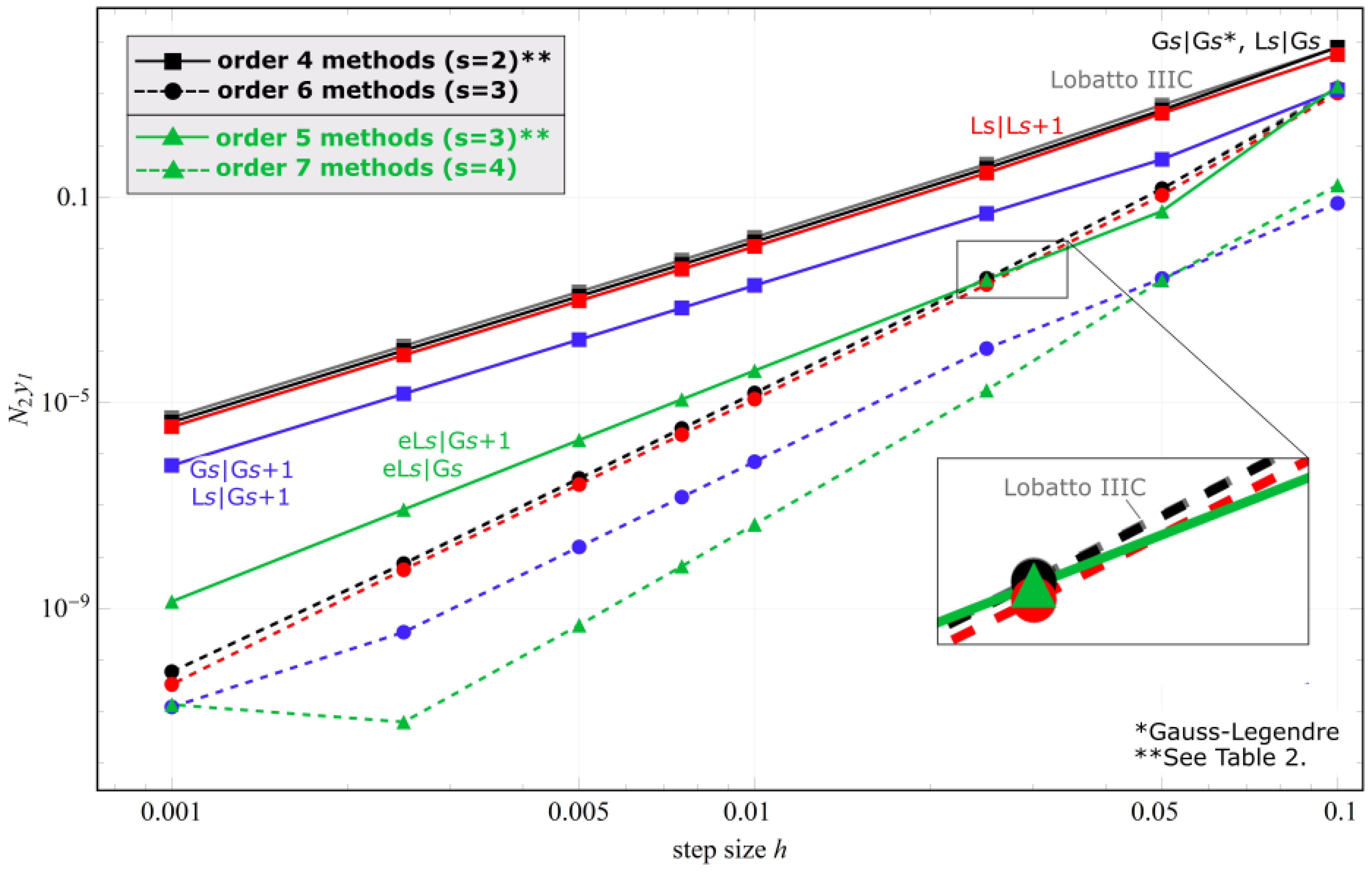
The differential equations describe the dynamic behavior of a mass–spring system. The mass is subject to a harmonic excitation and is oscillating about its static equilibrium. The particular excitation used adds high-frequency oscillations to the natural response of the mass, requiring a small step size and making the problem computationally demanding. The approximation errors of different methods for the variable are reported in Figure 1 with squares and circles for methods of order 4 and 6, respectively. In the same manner, the results for methods eLs|Gs and eLs|Gs+1 are denoted by triangles.
In Figure 1, Ls|Gs and Gs|Gs yielded the same error and, likewise, the Gs|Gs+1 and Ls|Gs+1 pair, as observed for all analyzed cases. The results demonstrate that the behavior of the new method seems to be determined by the integration rule on the right-hand side of the ODE. Gs|Gs+1 and Ls|Gs+1 also performed significantly better than the other methods. Ls|Ls+1 performed slightly better than Lobatto IIIC. A significant finding is that the usage of a different quadrature rule for the right-hand side of the ODE improved the accuracy of a numerical method.
Methods eLs|Gs and eLs|Gs+1 produced equivalent results in the analyzed example, as evident in Figure 1. Although they are of higher order (5 and 7) than the rest, they employ the same number of coefficients per variable (except Lobatto IIIC, which has a coefficient more than Gs|Gs at a given order of accuracy). For example, Gs|Gs of order 4 (G2|G2) employs two coefficients per variable, matching eLs|Gs at order 5; G3|G3 is of order 6 and employs three coefficients per variable and so does eL4|G4 at order 7. Although these methods share the same number of coefficients per step, a significant advantage of the “e” methods is observed.
Methods eLs|Gs and eLs|Gs+1 were applied only to Example 1. They require a very small step size for solving the remaining problems because they are not A-stable.
5.2. Example 2
The problem proposed by Frank and van der Houwen [23],
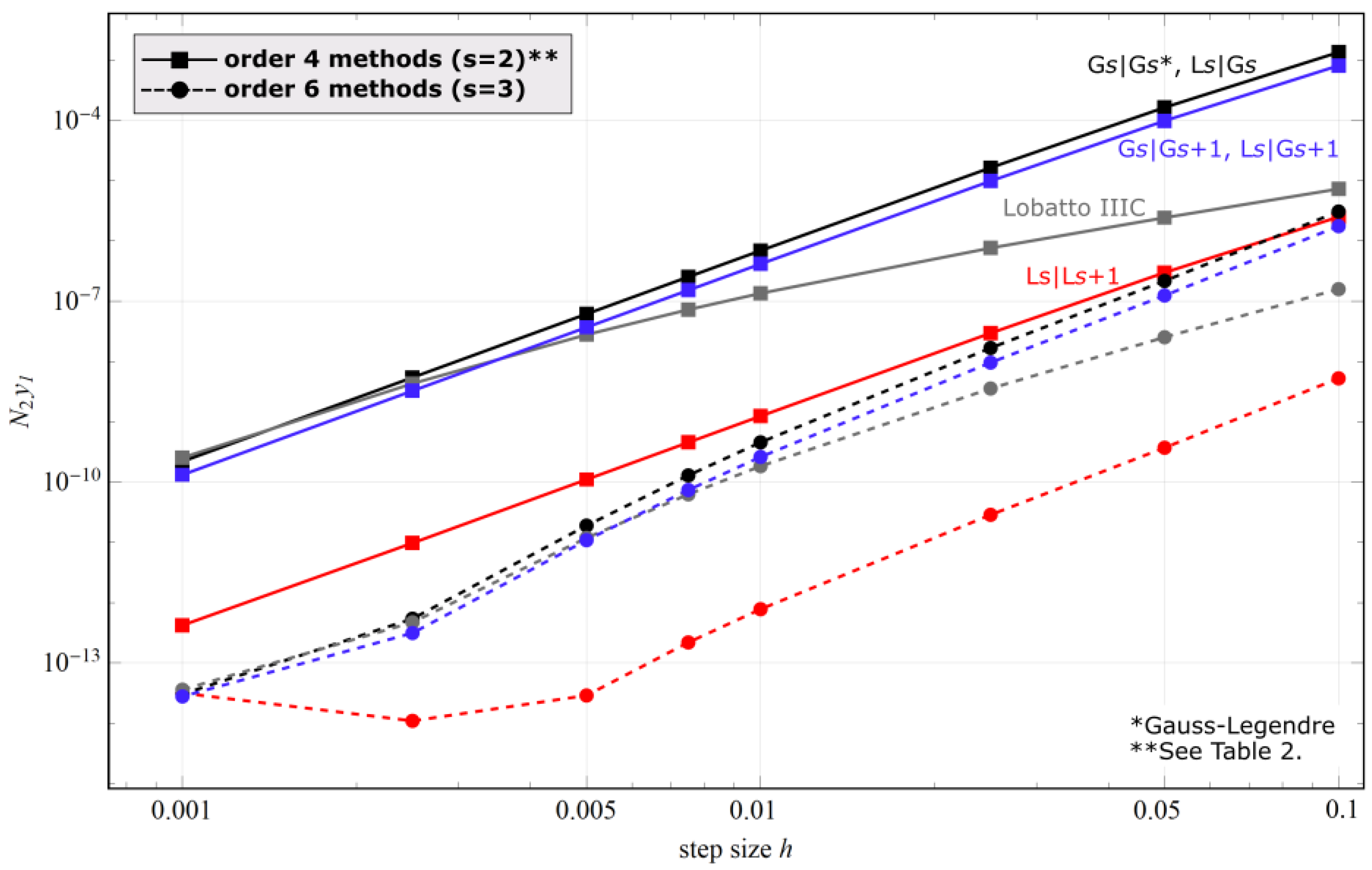
with exact solution , is a common choice for benchmarking [2,24]. Its intentionally designed stiffness is confirmed by computing the Jacobian of the right-hand side at the initial point and determining the eigenvalues , [2]. The computed errors of different methods for the variable are reported in Figure 2 with squares and circles for methods of order 4 and 6, respectively.
In Figure 2, Ls|Ls+1 outperformed the rest. The problem also seems to be suitable for the Lobatto IIIC, which performed better than Gs|Gs, Ls|Gs, Gs|Gs+1, and Ls|Gs+1. The latter two outperformed the Gs|Gs. However, while Ls|Gs, Gs|Gs+1, Ls|Gs+1, and Gs|Gs have the same number of unknown coefficients per step, Lobatto IIIC has a coefficient more per variable.
5.3. Example 3
A problem presented by Vigo-Aguiar et al. [2], and Frank and van der Houwen [23]:
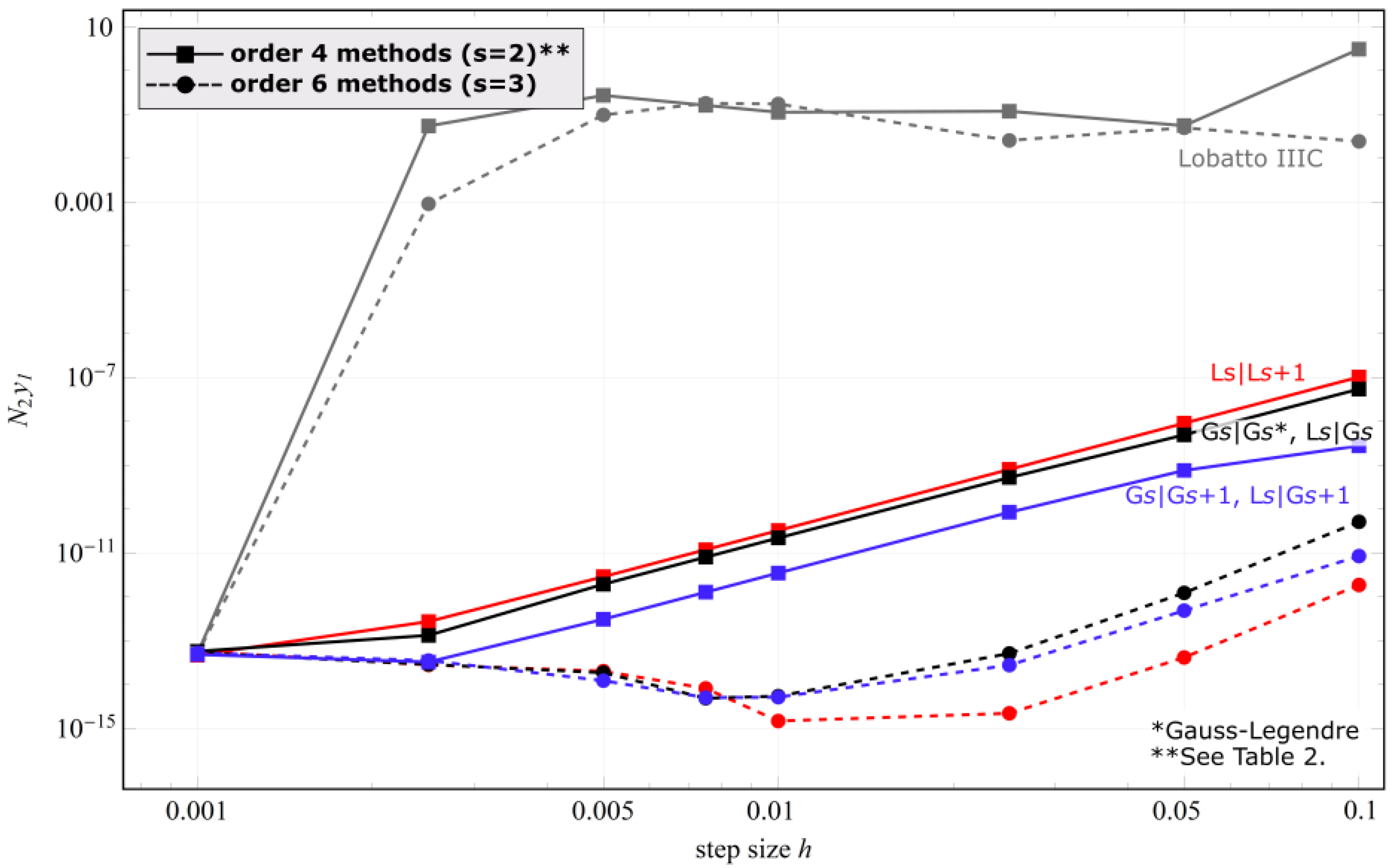
with the exact solution , and . The same highly stiff Jacobian matrix is computed as in the famous Robertson problem (describing the kinetics of three species), only altered by the nonhomogeneous terms [23]. The computed errors for the variable are reported in Figure 3 with squares and circles for methods of order 4 and 6, respectively.
In this problem (see Figure 3), Lobatto IIIC was unstable at larger step sizes. Among the methods of order 4, L2|G3 and G2|G3 performed best, while L3|L4 seemed to be the most appropriate order 6 method.
5.4. Example 4
The problem presented by Vigo-Aguiar et al. [2], and Frank and van der Houwen [23]:
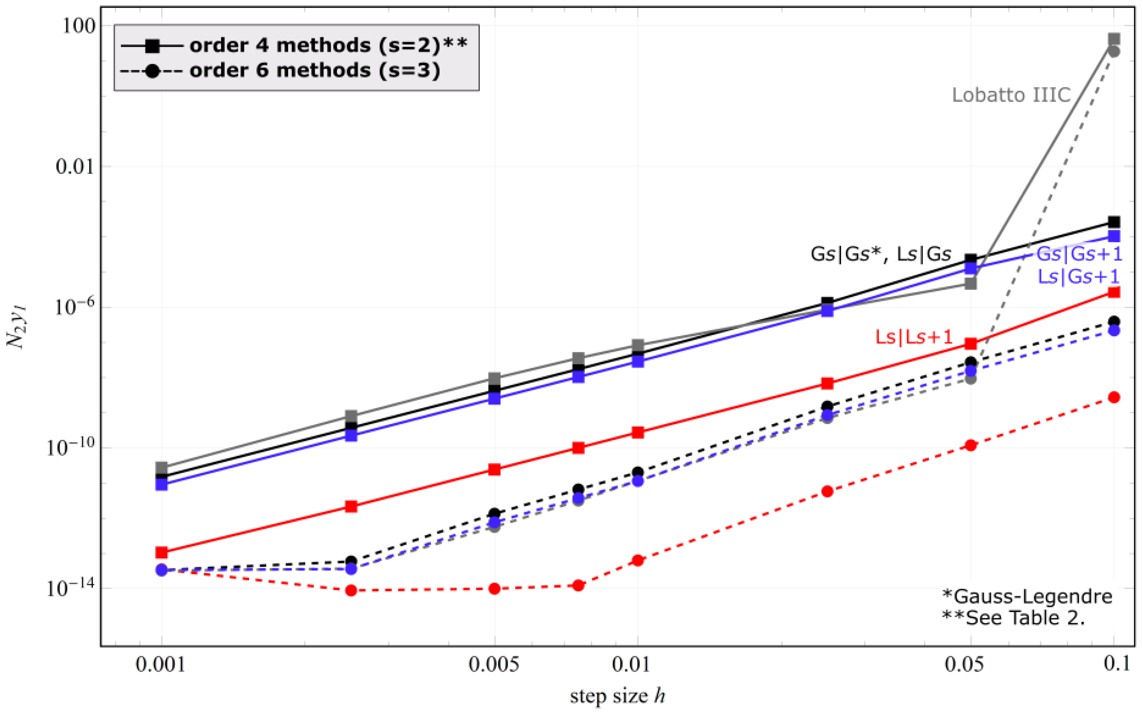
with exact solution , . This is a more computationally intensive test problem due to strong nonlinearity. The approximation errors of different methods for the variable are reported in Figure 4 with squares and circles for methods of order 4 and 6, respectively. The best was Ls|Ls+1, followed by Ls|Gs+1 and Gs|Gs+1, and then Gs|Gs.
6. Discussion
The results show that changing the quadrature rule for the left-hand side of differential Equation (4) had a minuscule effect on the results. However, increasing the order on the right-hand side, i.e., methods #s|#s+1, improved the accuracy at the same number of coefficients. This was demonstrated on test equations analytically, as well as on some numerical examples.
In contrast to the classical derivation of collocation RK-type methods, the new method class is derived from the integral form of the ODE. This approach allows integrating the left-hand and the right-hand side separately, enabling us to employ different quadrature rules for each, resulting in a multitude of method families. Proof is provided that using Gauss quadrature on both ODE sides results in the Gauss–Legendre method and, likewise, Lobatto quadrature returns the Lobatto IIIA method.
By examining the computational cost of the analyzed methods for the presented examples (data not shown), the Gauss–Legendre method somewhat outperformed the proposed methods whereas the Lobatto method was the slowest. However, despite producing computationally somewhat inefficient results, we still believe that the presented approach contributes to our understanding of RK-type collocation methods; it shows how their accuracy can be enhanced (for the same number of method’s coefficients) and presents a new way of constructing them.
The proposed method class was found to be especially suitable for (high-frequency) oscillatory and stiff problems. We compared certain novel subclasses to implicit RK-type methods, i.e., the established collocation methods with the same framework and purpose, and we demonstrated the advantage of the new methods. Certain extensions and alternatives could outperform the proposed approach: the embedded formula collocation method [20,25], multivalue methods [26], parallel time integration methods [27], variable step size methods [28], block methods [29,30,31,32], etc. We focused on the popular RK-type methods to avoid an extensive comparison to all the possible alternatives. Tables similar to Butcher tableaus are provided for convenience and comparison to the RK methods. The behavior of methods was in this work demonstrated on some of the well-known ODEs from literature. These include stiff problems, as well as a nonlinear and highly oscillatory system. Systems where the accuracy of methods can behave differently, such as chaotic-type problems [33] or DAE systems [14], are beyond the scope of this work.
Although the implicit RK methods are known to be computationally expensive, much effort has been devoted to developing effective numerical algorithms and efficient computer software packages [3]. Well-known solvers based on the implicit RK approach are RADAU, STRIDE, DIRK, and SDIRK, popular for integrating stiff systems. Implicit RK methods can employ a much larger step size than the explicit ones. The relatively small interval of absolute stability makes the explicit RK methods unsuitable for stiff initial value problems [6]. The presented approach allows improving the implicit RK by increasing the integration accuracy of the right-hand side of the ODE at no additional computational cost.
7. Conclusions
A new class of methods for numerical integration of ODEs was proposed. The methods allow the usage of differing quadrature rules for the integration of the right-hand side of ODEs while using the same approximation function for the solution of the ODE. We demonstrated how the accuracy of Gauss–Legendre and Lobatto IIIA methods, which can also be derived from the proposed approach, can be increased at the same number of method stages.
In engineering and natural sciences, implicit RK-type methods are still widely used, especially for solving stiff systems [34,35]. As researchers are familiar with Butcher tableaus, the existing program codes can be enhanced in accuracy according to the proposed approach by forming an altered set of equations which is a rather small modification that retains the number of unknowns.
More methods of the novel class remain to be analyzed. For the sake of clarity, in this work, we only analyzed the Gauss–Legendre and Lobatto collocation points. Several more options are available, such as the Radau I, Radau II, or the so-called Gauss–Lobatto Chebyshev points. These would yield different method instances, further extending the investigation. The optimal choice for the quadrature on the right-hand side still remains to be determined.
Supplementary Materials
The following are available online at https://www.mdpi.com/2227-7390/9/2/174/s1, Tableaus for the proposed families of methods (provided in the form of analytical expressions), Tables S1–S21.
Author Contributions
Conceptualization, J.U.; methodology, J.U. and M.H.; validation, J.U. and M.H.; writing—original draft preparation, J.U. and M.H.; writing—review and editing, J.U. and M.H.; supervision, M.H.; project administration, M.H. All authors read and agreed to the published version of the manuscript.
Funding
The authors acknowledge financial support from the Slovenian Research Agency (research core funding No. P2-0263).
Institutional Review Board Statement
Not applicable.
Informed Consent Statement
Not applicable.
Data Availability Statement
Not applicable.
Conflicts of Interest
The authors declare no conflict of interest.
Appendix A
Below, tableaus for some of the presented families of methods (with s = 2, 3, 4) are provided in the form of analytical expressions. A complete set of tableaus is provided in the Supplementary Materials. The tables include Table A1, Table A2 and Table A3: tableaus for the Gs|Gs method, Table A4, Table A5 and Table A6: tableaus for the Ls|Ls method, and Table A7, Table A8 and Table A9: tableaus for the Ls|Ls+1 method.

Table A1.
G2|G2 method.
, .
Table A2.
G3|G3 method.
, , , .
Table A3.
G4|G4 method.
, , , , , , .
Table A4.
L2|L2 method.
Table A5.
L3|L3 method.
Table A6.
L4|L4 method.
, , , .
Table A7.
L2|L3 method.
Table A8.
L3|L4 method.
, , , .
Table A9.
L4|L5 method.
| 0 | ||||||||
| 0 | 0 | 0 | 0 | |||||
, , , , , .
Appendix B
Below, tableaus for the proposed families of methods (with s = 2, 3, 4) are provided in the form of numerical values. Tables include Table A10, Table A11 and Table A12: tableaus for the Gs|Gs method, Table A13, Table A14 and Table A15: tableaus for the Gs|Gs+1 method, Table A16, Table A17 and Table A18: tableaus for the Ls|Ls method, Table A19, Table A20 and Table A21: tableaus for the Ls|Ls+1 method, Table A22, Table A23 and Table A24: tableaus for the Ls|Gs+1 method, Table A25, Table A26 and Table A27: tableaus for the eLs|Gs method, and Table A28, Table A29 and Table A30: tableaus for the eLs|Gs+1 method.
Table A10.
G2|G2 method.
| 0.3943375673 | 0.1056624327 | 0.3943375673 | 0.1056624327 |
| 0.1056624327 | 0.3943375673 | 0.1056624327 | 0.3943375673 |
| 0.2500000000 | −0.0386751346 | ||
| 0.5386751346 | 0.2500000000 | ||
| 0.5000000000 | 0.5000000000 | 0.2113248654 | 0.7886751346 |
Table A11.
G3|G3 method.
| 0.1909162041 | 0.0000000000 | −0.0242495374 | 0.1909162041 | 0.0000000000 | −0.0242495374 |
| 0.1111111111 | 0.4444444444 | 0.1111111111 | 0.1111111111 | 0.4444444444 | 0.1111111111 |
| −0.0242495374 | 0.0000000000 | 0.1909162041 | −0.0242495374 | 0.0000000000 | 0.1909162041 |
| 0.1388888889 | −0.0359766675 | 0.0097894440 | |||
| 0.3002631950 | 0.2222222222 | −0.0224854172 | |||
| 0.2679883338 | 0.4804211120 | 0.1388888889 | |||
| 0.2777777778 | 0.4444444444 | 0.2777777778 | 0.1127016654 | 0.5000000000 | 0.8872983346 |
Table A12.
G4|G4 method.
| 0.1095643912 | −0.0230516341 | −0.0113542767 | 0.0081748529 | 0.1095643912 | −0.0230516341 | −0.0113542767 | 0.0081748529 |
| 0.0821909249 | 0.3172608528 | 0.0432176354 | −0.0260027464 | 0.0821909249 | 0.3172608528 | 0.0432176354 | −0.0260027464 |
| −0.0260027464 | 0.0432176354 | 0.3172608528 | 0.0821909249 | −0.0260027464 | 0.0432176354 | 0.3172608528 | 0.0821909249 |
| 0.0081748529 | −0.0113542767 | −0.0230516341 | 0.1095643912 | 0.0081748529 | −0.0113542767 | −0.0230516341 | 0.1095643912 |
| 0.0869637113 | −0.0266041801 | 0.0126274627 | −0.0035551497 | ||||
| 0.1881181175 | 0.1630362887 | −0.0278804286 | 0.0067355006 | ||||
| 0.1671919220 | 0.3539530060 | 0.1630362887 | −0.0141906949 | ||||
| 0.1774825723 | 0.3134451147 | 0.3526767575 | 0.0869637113 | ||||
| 0.1739274226 | 0.3260725774 | 0.3260725774 | 0.1739274226 | 0.0694318442 | 0.3300094782 | 0.6699905218 | 0.9305681558 |
Table A13.
G2|G3 method.
| 0.3943375673 | 0.1056624327 | 0.2464717596 | 0.2222222222 | 0.0313060182 |
| 0.1056624327 | 0.3943375673 | 0.0313060182 | 0.2222222222 | 0.2464717596 |
| 0.1429533731 | −0.0302517077 | |||
| 0.4665063509 | 0.0334936491 | |||
| 0.5302517077 | 0.3570466269 | |||
| 0.5000000000 | 0.5000000000 | 0.1127016654 | 0.5000000000 | 0.8872983346 |
Table A14.
G3|G4 method.
| 0.1909162041 | 0.0000000000 | −0.0242495374 | 0.1393760495 | 0.0742741410 | −0.0365843541 | −0.0103991697 |
| 0.1111111111 | 0.4444444444 | 0.1111111111 | 0.0449505428 | 0.2883827906 | 0.2883827906 | 0.0449505428 |
| −0.0242495374 | 0.0000000000 | 0.1909162041 | −0.0103991697 | −0.0365843541 | 0.0742741410 | 0.1393760495 |
| 0.0919034035 | −0.0309624389 | 0.0084908796 | ||||
| 0.2761524294 | 0.0631476522 | −0.0092906034 | ||||
| 0.2870683812 | 0.3812967923 | 0.0016253483 | ||||
| 0.2692868982 | 0.4754068833 | 0.1858743743 | ||||
| 0.2777777778 | 0.4444444444 | 0.2777777778 | 0.0694318442 | 0.3300094782 | 0.6699905218 | 0.9305681558 |
Table A15.
G4|G5 method.
| 0.1095643912 | −0.0230516341 | −0.0113542767 | 0.0081748529 | 0.0876663770 | 0.0206983089 | −0.0355555556 | 0.0062093567 | 0.0043148463 |
| 0.0821909249 | 0.3172608528 | 0.0432176354 | −0.0260027464 | 0.0400713018 | 0.2340778829 | 0.1777777778 | −0.0216712133 | −0.0135890825 |
| −0.0260027464 | 0.0432176354 | 0.3172608528 | 0.0821909249 | −0.0135890825 | −0.0216712133 | 0.1777777778 | 0.2340778829 | 0.0400713018 |
| 0.0081748529 | −0.0113542767 | −0.0230516341 | 0.1095643912 | 0.0043148463 | 0.0062093567 | −0.0355555556 | 0.0206983089 | 0.0876663770 |
| 0.0627027106 | −0.0240331396 | 0.0114763336 | −0.0032358275 | |||||
| 0.1782025822 | 0.0646259362 | −0.0159331476 | 0.0038699741 | |||||
| 0.1761059379 | 0.3049159395 | 0.0211566379 | −0.0021785154 | |||||
| 0.1700574485 | 0.3420057250 | 0.2614466412 | −0.0042751596 | |||||
| 0.1771632501 | 0.3145962439 | 0.3501057171 | 0.1112247120 | |||||
| 0.1739274226 | 0.3260725774 | 0.3260725774 | 0.1739274226 | 0.0469100770 | 0.2307653449 | 0.5000000000 | 0.7692346551 | 0.9530899230 |
Table A16.
L2|L2 method.
| 0.3333333333 | 0.1666666667 | 0.3333333333 | 0.1666666667 |
| 0.1666666667 | 0.3333333333 | 0.1666666667 | 0.3333333333 |
| 0.0000000000 | 0.0000000000 | ||
| 0.5000000000 | 0.5000000000 | ||
| 0.5000000000 | 0.5000000000 | 0.0000000000 | 1.0000000000 |
Table A17.
L3|L3 method.
| 0.1333333333 | 0.0666666667 | −0.0333333333 | 0.1333333333 | 0.0666666667 | −0.0333333333 |
| 0.0666666667 | 0.5333333333 | 0.0666666667 | 0.0666666667 | 0.5333333333 | 0.0666666667 |
| −0.0333333333 | 0.0666666667 | 0.1333333333 | −0.0333333333 | 0.0666666667 | 0.1333333333 |
| 0.0000000000 | 0.0000000000 | 0.0000000000 | |||
| 0.2083333333 | 0.3333333333 | −0.0416666667 | |||
| 0.1666666667 | 0.6666666667 | 0.1666666667 | |||
| 0.1666666667 | 0.6666666667 | 0.1666666667 | 0.0000000000 | 0.5000000000 | 1.0000000000 |
Table A18.
L4|L4 method.
| 0.0714285714 | 0.0266198569 | −0.0266198569 | 0.0119047619 | 0.0714285714 | 0.0266198569 | −0.0266198569 | 0.0119047619 |
| 0.0266198569 | 0.3571428571 | 0.0595238095 | −0.0266198569 | 0.0266198569 | 0.3571428571 | 0.0595238095 | −0.0266198569 |
| −0.0266198569 | 0.0595238095 | 0.3571428571 | 0.0266198569 | −0.0266198569 | 0.0595238095 | 0.3571428571 | 0.0266198569 |
| 0.0119047619 | −0.0266198569 | 0.0266198569 | 0.0714285714 | 0.0119047619 | −0.0266198569 | 0.0266198569 | 0.0714285714 |
| 0.0000000000 | 0.0000000000 | 0.0000000000 | 0.0000000000 | ||||
| 0.1103005665 | 0.1896994335 | −0.0339073642 | 0.0103005665 | ||||
| 0.0730327669 | 0.4505740309 | 0.2269672331 | −0.0269672331 | ||||
| 0.0833333333 | 0.4166666667 | 0.4166666667 | 0.0833333333 | ||||
| 0.0833333333 | 0.4166666667 | 0.4166666667 | 0.0833333333 | 0.0000000000 | 0.2763932023 | 0.7236067977 | 1.0000000000 |
Table A19.
L2|L3 method.
| 0.3333333333 | 0.1666666667 | 0.1666666667 | 0.3333333333 | 0.0000000000 |
| 0.1666666667 | 0.3333333333 | 0.0000000000 | 0.3333333333 | 0.1666666667 |
| 0.0000000000 | 0.0000000000 | |||
| 0.3750000000 | 0.1250000000 | |||
| 0.5000000000 | 0.5000000000 | |||
| 0.5000000000 | 0.5000000000 | 0.0000000000 | 0.5000000000 | 1.0000000000 |
Table A20.
L3|L4 method.
| 0.1333333333 | 0.0666666667 | −0.0333333333 | 0.0833333333 | 0.1348361657 | −0.0515028324 | 0.0000000000 |
| 0.0666666667 | 0.5333333333 | 0.0666666667 | 0.0000000000 | 0.3333333333 | 0.3333333333 | 0.0000000000 |
| −0.0333333333 | 0.0666666667 | 0.1333333333 | 0.0000000000 | −0.0515028324 | 0.1348361657 | 0.0833333333 |
| 0.0000000000 | 0.0000000000 | 0.0000000000 | ||||
| 0.1758797734 | 0.1246336554 | −0.0241202266 | ||||
| 0.1907868933 | 0.5420330112 | −0.0092131067 | ||||
| 0.1666666667 | 0.6666666667 | 0.1666666667 | ||||
| 0.1666666667 | 0.6666666667 | 0.1666666667 | 0.0000000000 | 0.2763932023 | 0.7236067977 | 1.0000000000 |
Table A21.
L4|L5 method.
| 0.0714285714 | 0.0266198569 | −0.0266198569 | 0.0119047619 | 0.0500000000 | 0.0643476427 | −0.0444444444 | 0.0134301350 | 0.0000000000 |
| 0.0266198569 | 0.3571428571 | 0.0595238095 | −0.0266198569 | 0.0000000000 | 0.2395409829 | 0.2222222222 | −0.0450965384 | 0.0000000000 |
| −0.0266198569 | 0.0595238095 | 0.3571428571 | 0.0266198569 | 0.0000000000 | −0.0450965384 | 0.2222222222 | 0.2395409829 | 0.0000000000 |
| 0.0119047619 | −0.0266198569 | 0.0266198569 | 0.0714285714 | 0.0000000000 | 0.0134301350 | −0.0444444444 | 0.0643476427 | 0.0500000000 |
| 0.0000000000 | 0.0000000000 | 0.0000000000 | 0.0000000000 | |||||
| 0.0992752781 | 0.0900222220 | −0.0240628789 | 0.0074385434 | |||||
| 0.0885416667 | 0.3830261441 | 0.0336405226 | −0.0052083333 | |||||
| 0.0758947899 | 0.4407295456 | 0.3266444447 | −0.0159419448 | |||||
| 0.0833333333 | 0.4166666667 | 0.4166666667 | 0.0833333333 | |||||
| 0.0833333333 | 0.4166666667 | 0.4166666667 | 0.0833333333 | 0.0000000000 | 0.1726731646 | 0.5000000000 | 0.8273268354 | 1.0000000000 |
Table A22.
L2|G3 method.
| 0.3333333333 | .1666666667 | 0.2464717596 | 0.2222222222 | 0.0313060182 |
| 0.1666666667 | 0.3333333333 | 0.0313060182 | 0.2222222222 | 0.2464717596 |
| 0.1063508327 | 0.0063508327 | |||
| 0.3750000000 | 0.1250000000 | |||
| 0.4936491673 | 0.3936491673 | |||
| 0.5000000000 | 0.5000000000 | 0.1127016654 | 0.5000000000 | 0.8872983346 |
Table A23.
L3|G4 method.
| 0.1333333333 | 0.0666666667 | −0.0333333333 | 0.1393760495 | 0.0742741410 | −0.0365843541 | −0.0103991697 |
| 0.0666666667 | 0.5333333333 | 0.0666666667 | 0.0449505428 | 0.2883827906 | 0.2883827906 | 0.0449505428 |
| −0.0333333333 | 0.0666666667 | 0.1333333333 | −0.0103991697 | −0.0365843541 | 0.0742741410 | 0.1393760495 |
| 0.0624238165 | 0.0091952744 | −0.0021872467 | ||||
| 0.1906101591 | 0.1698923826 | −0.0304930634 | ||||
| 0.1971597301 | 0.4967742841 | −0.0239434924 | ||||
| 0.1688539134 | 0.6574713923 | 0.1042428501 | ||||
| 0.1666666667 | 0.6666666667 | 0.1666666667 | 0.0694318442 | 0.3300094782 | 0.6699905218 | 0.9305681558 |
Table A24.
L4|G5 method.
| 0.0714285714 | 0.0266198569 | −0.0266198569 | 0.0119047619 | 0.0876663770 | 0.0206983089 | −0.0355555556 | 0.0062093567 | 0.0043148463 |
| 0.0266198569 | 0.3571428571 | 0.0595238095 | −0.0266198569 | 0.0400713018 | 0.2340778829 | 0.1777777778 | −0.0216712133 | −0.0135890825 |
| −0.0266198569 | 0.0595238095 | 0.3571428571 | 0.0266198569 | −0.0135890825 | −0.0216712133 | 0.1777777778 | 0.2340778829 | 0.0400713018 |
| 0.0119047619 | −0.0266198569 | 0.0266198569 | 0.0714285714 | 0.0043148463 | 0.0062093567 | −0.0355555556 | 0.0206983089 | 0.0876663770 |
| 0.0406464521 | 0.0082518815 | −0.0029225402 | 0.0009342837 | |||||
| 0.1084254894 | 0.1444003333 | −0.0317501637 | 0.0096896860 | |||||
| 0.0885416667 | 0.3830261441 | 0.0336405226 | −0.0052083333 | |||||
| 0.0736436474 | 0.4484168303 | 0.2722663333 | −0.0250921560 | |||||
| 0.0823990496 | 0.4195892069 | 0.4084147852 | 0.0426868813 | |||||
| 0.0833333333 | 0.4166666667 | 0.4166666667 | 0.0833333333 | 0.0469100770 | 0.2307653449 | 0.5000000000 | 0.7692346551 | 0.9530899230 |
Table A25.
eL2|G2 method.
| 0.5000000000 | 0.5000000000 | 0.5000000000 | 0.5000000000 |
| 0.1889957660 | 0.0223290994 | ||
| 0.4776709006 | 0.3110042340 | ||
| 0.5000000000 | 0.5000000000 | 0.2113248654 | 0.7886751346 |
Table A26.
eL3|G3 method.
| 0.1666666667 | 0.3333333333 | 0.0000000000 | 0.2464717596 | 0.2222222222 | 0.0313060182 |
| 0.0000000000 | 0.3333333333 | 0.1666666667 | 0.0313060182 | 0.2222222222 | 0.2464717596 |
| 0.0946034999 | 0.0234946656 | −0.0053965001 | |||
| 0.2083333333 | 0.3333333333 | −0.0416666667 | |||
| 0.1720631668 | 0.6431720010 | 0.0720631668 | |||
| 0.1666666667 | 0.6666666667 | 0.1666666667 | 0.1127016654 | 0.5000000000 | 0.8872983346 |
Table A27.
eL4|G4 method.
| 0.0833333333 | 0.1348361657 | −0.0515028324 | 0.0000000000 | 0.1393760495 | 0.0742741410 | −0.0365843541 | −0.0103991697 |
| 0.0000000000 | 0.3333333333 | 0.3333333333 | 0.0000000000 | 0.0449505428 | 0.2883827906 | 0.2883827906 | 0.0449505428 |
| 0.0000000000 | −0.0515028324 | 0.1348361657 | 0.0833333333 | −0.0103991697 | −0.0365843541 | 0.0742741410 | 0.1393760495 |
| 0.0560561704 | 0.0174153788 | −0.0059212859 | 0.0018815809 | ||||
| 0.1082653175 | 0.2428250379 | −0.0304595597 | 0.0093786825 | ||||
| 0.0739546508 | 0.4471262264 | 0.1738416287 | −0.0249319842 | ||||
| 0.0814517525 | 0.4225879525 | 0.3992512878 | 0.0272771630 | ||||
| 0.0833333333 | 0.4166666667 | 0.4166666667 | 0.0833333333 | 0.0694318442 | 0.3300094782 | 0.6699905218 | 0.9305681558 |
Table A28.
eL2|G3 method.
| 0.5000000000 | 0.5000000000 | 0.2777777778 | 0.4444444444 | 0.2777777778 |
| 0.1063508327 | 0.0063508327 | |||
| 0.3750000000 | 0.1250000000 | |||
| 0.4936491673 | 0.3936491673 | |||
| 0.5000000000 | 0.5000000000 | 0.1127016654 | 0.5000000000 | 0.8872983346 |
Table A29.
eL3|G4 method.
| 0.1666666667 | 0.3333333333 | 0.0000000000 | 0.1618513209 | 0.2184655363 | 0.1076070411 | 0.0120761017 |
| 0.0000000000 | 0.3333333333 | 0.1666666667 | 0.0120761017 | 0.1076070411 | 0.2184655363 | 0.1618513209 |
| 0.0624238165 | 0.0091952744 | −0.0021872467 | ||||
| 0.1906101591 | 0.1698923826 | −0.0304930634 | ||||
| 0.1971597301 | 0.4967742841 | −0.0239434924 | ||||
| 0.1688539134 | 0.6574713923 | 0.1042428501 | ||||
| 0.1666666667 | 0.6666666667 | 0.1666666667 | 0.0694318442 | 0.3300094782 | 0.6699905218 | 0.9305681558 |
Table A30.
eL4|G5 method.
| 0.0833333333 | 0.1348361657 | −0.0515028324 | 0.0000000000 | 0.1023134256 | 0.0991262123 | 0.0000000000 | −0.0297372127 | −0.0050357585 |
| 0.0000000000 | 0.3333333333 | 0.3333333333 | 0.0000000000 | 0.0211857754 | 0.1699253357 | 0.2844444444 | 0.1699253357 | 0.0211857754 |
| 0.0000000000 | −0.0515028324 | 0.1348361657 | 0.0833333333 | −0.0050357585 | −0.0297372127 | 0.0000000000 | 0.0991262123 | 0.1023134256 |
| 0.0406464521 | 0.0082518815 | −0.0029225402 | 0.0009342837 | |||||
| 0.1084254894 | 0.1444003333 | −0.0317501637 | 0.0096896860 | |||||
| 0.0885416667 | 0.3830261441 | 0.0336405226 | −0.0052083333 | |||||
| 0.0736436474 | 0.4484168303 | 0.2722663333 | −0.0250921560 | |||||
| 0.0823990496 | 0.4195892069 | 0.4084147852 | 0.0426868813 | |||||
| 0.0833333333 | 0.4166666667 | 0.4166666667 | 0.0833333333 | 0.0469100770 | 0.2307653449 | 0.5000000000 | 0.7692346551 | 0.9530899230 |
References
- Chan, Y.N.I.; Birnbaum, I.; Lapidus, L. Solution of Stiff Differential Equations and the Use of Imbedding Techniques. Ind. Eng. Chem. Fund. 1978, 17, 133–148. [Google Scholar] [CrossRef]
- Vigo-Aguiar, J.; Martín-Vaquero, J.; Ramos, H. Exponential Fitting BDF–Runge–Kutta Algorithms. Comput. Phys. Commun. 2008, 178, 15–34. [Google Scholar] [CrossRef]
- Martín-Vaquero, J. A 17th-Order Radau IIA Method for Package RADAU. Applications in Mechanical Systems. Comput. Math. Appl. 2010, 59, 2464–2472. [Google Scholar] [CrossRef] [Green Version]
- Cash, J.R. Review Paper: Efficient Numerical Methods for the Solution of Stiff Initial-Value Problems and Differential Algebraic Equations. Proc. R. Soc. Lond. A 2003, 459, 797–815. [Google Scholar] [CrossRef]
- Costabile, F.; Napoli, A. A Class of Collocation Methods for Numerical Integration of Initial Value Problems. Comput. Math. Appl. 2011, 62, 3221–3235. [Google Scholar] [CrossRef] [Green Version]
- Ying, T.Y.; Yaacob, N. Implicit 7-Stage Tenth Order Runge-Kutta Methods Based on Gauss-Kronrod-Lobatto Quadrature Formula. Malays. J. Ind. Appl. Math. 2015, 31, 17. [Google Scholar]
- Perez-Rodriguez, S.; Gonzalez-Pinto, S.; Sommeijer, B.P. An Iterated Radau Method for Time-Dependent PDEs. J. Comput. Appl. Math. 2009, 231, 49–66. [Google Scholar] [CrossRef] [Green Version]
- Ramos, H.; García-Rubio, R. Analysis of a Chebyshev-Based Backward Differentiation Formulae and Relation with Runge–Kutta Collocation Methods. Int. J. Comput. Math. 2011, 88, 555–577. [Google Scholar] [CrossRef]
- Vigo-Aguiar, J.; Ramos, H. A New Eighth-Order A-Stable Method for Solving Differential Systems Arising in Chemical Reactions. J. Math. Chem. 2006, 40, 71–83. [Google Scholar] [CrossRef]
- Ying, T.Y.; Yaacob, N. Numerical Solution of First Order Initial Value Problem Using 5-Stage Eighth Order Gauss-Kronrod Method. World Appl. Sci. J. 2013, 21, 1017–1024. [Google Scholar]
- Ying, T.Y.; Yaacob, N. Two Classes of Implicit Runge-Kutta Methods Based on Gauss-Kronrod-Radau Quadrature Formulae. Discov. Math. 2013, 35, 1–14. [Google Scholar]
- Liu, H.; Sun, G. Implicit Runge–Kutta Methods Based on Lobatto Quadrature Formula. Int. J. Comput. Math. 2005, 82, 77–88. [Google Scholar] [CrossRef]
- Butcher, J.C. Numerical Methods for Ordinary Differential Equations, 2nd ed.; Wiley: Chichester, England; Hoboken, NJ, USA, 2008; ISBN 978-0-470-72335-7. [Google Scholar]
- Jay, L. Convergence of a Class of Runge-Kutta Methods for Differential-Algebraic Systems of Index 2. BIT Numer. Math. 1993, 33, 137–150. [Google Scholar] [CrossRef]
- Jay, L. Symplectic Partitioned Runge–Kutta Methods for Constrained Hamiltonian Systems. Siam J. Numer. Anal. 1996, 33, 368–387. [Google Scholar] [CrossRef]
- Hairer, E.; Wanner, G. Radau Methods. In Encyclopedia of Applied and Computational Mathematics; Engquist, B., Ed.; Springer: Berlin/Heidelberg, Germany, 2015; pp. 1213–1216. ISBN 978-3-540-70528-4. [Google Scholar]
- Atkinson, K.; Weimin, H. Elementary Numerical Analysis, 3rd ed.; John Wiley: New York, NY, USA, 2003. [Google Scholar]
- Hairer, E.; Nørsett, S.P.; Wanner, G. Solving Ordinary Differential Equations I: Nonstiff Problems; Springer Series in Computational Mathematics; Springer: Berlin/Heidelberg, Germany, 1993; Volume 8, ISBN 978-3-540-56670-0. [Google Scholar]
- Butcher, J.C. Integration Processes Based on Radau Quadrature Formulas. Math. Comp. 1964, 18, 233–244. [Google Scholar] [CrossRef]
- Hairer, E.; Wanner, G. Solving Ordinary Differential Equations II: Stiff and Differential-Algebraic Problems, 2nd ed.; Springer Series in Computational Mathematics; Springer: Berlin/Heidelberg, Germany, 1996; ISBN 978-3-540-60452-5. [Google Scholar]
- Butcher, J.C. Implicit Runge-Kutta Processes. Math. Comput. 1964, 18, 15. [Google Scholar] [CrossRef]
- Jay, L.O. Lobatto Methods. In Encyclopedia of Applied and Computational Mathematics; Engquist, B., Ed.; Springer: Berlin/Heidelberg, Germany, 2015; ISBN 978-3-540-70528-4. [Google Scholar]
- Frank, J.E.; van der Houwen, P.J. Parallel Iteration of the Extended Backward Differentiation Formulas. Ima J. Numer. Anal. 2001, 21, 367–385. [Google Scholar] [CrossRef]
- Sami Bataineh, A.; Noorani, M.S.M.; Hashim, I. Solving Systems of ODEs by Homotopy Analysis Method. Commun. Nonlinear Sci. Numer. Simul. 2008, 13, 2060–2070. [Google Scholar] [CrossRef]
- Piao, X.; Bu, S.; Kim, D.; Kim, P. An Embedded Formula of the Chebyshev Collocation Method for Stiff Problems. J. Comput. Phys. 2017, 351, 376–391. [Google Scholar] [CrossRef]
- D’Ambrosio, R.; Paternoster, B. Multivalue Collocation Methods Free from Order Reduction. J. Comput. Appl. Math. 2021, 387, 112515. [Google Scholar] [CrossRef]
- Gander, M.J. 50 Years of Time Parallel Time Integration. In Multiple Shooting and Time Domain Decomposition Methods; Carraro, T., Geiger, M., Körkel, S., Rannacher, R., Eds.; Springer International Publishing: Cham, Switzerland, 2015; pp. 69–113. [Google Scholar]
- Vigo-Aguiar, J.; Ramos, H. A Family of A-Stable Runge Kutta Collocation Methods of Higher Order for Initial-Value Problems. Ima J. Numer. Anal. 2007, 27, 798–817. [Google Scholar] [CrossRef]
- Singh, G.; Garg, A.; Kanwar, V.; Ramos, H. An Efficient Optimized Adaptive Step-Size Hybrid Block Method for Integrating Differential Systems. Appl. Math. Comput. 2019, 362, 124567. [Google Scholar] [CrossRef]
- Ramos, H.; Rufai, M.A. Third Derivative Modification of K-Step Block Falkner Methods for the Numerical Solution of Second Order Initial-Value Problems. Appl. Math. Comput. 2018, 333, 231–245. [Google Scholar] [CrossRef]
- Modebei, M.I.; Adeniyi, R.B.; Jator, S.N.; Ramos, H. A Block Hybrid Integrator for Numerically Solving Fourth-Order Initial Value Problems. Appl. Math. Comput. 2019, 346, 680–694. [Google Scholar] [CrossRef]
- Ibrahim, Z.B.; Nasarudin, A.A. A Class of Hybrid Multistep Block Methods with A–Stability for the Numerical Solution of Stiff Ordinary Differential Equations. Mathematics 2020, 8, 914. [Google Scholar] [CrossRef]
- Lozi, R.; Pchelintsev, A.N. A New Reliable Numerical Method for Computing Chaotic Solutions of Dynamical Systems: The Chen Attractor Case. Int. J. Bifurc. Chaos 2015, 25, 1550187. [Google Scholar] [CrossRef] [Green Version]
- Adeyeye, O.; Omar, Z. Implicit Five-Step Block Method with Generalised Equidistant Points for Solving Fourth Order Linear and Non-Linear Initial Value Problems. Ain Shams Eng. J. 2019, 10, 881–889. [Google Scholar] [CrossRef]
- Ramos, H.; Patricio, M.F. Some New Implicit Two-Step Multiderivative Methods for Solving Special Second-Order IVP’s. Appl. Math. Comput. 2014, 239, 227–241. [Google Scholar] [CrossRef]
Figure 1.
The error of different methods (as the norm) vs. the step size in Example 1 (log–log scale). The method accuracy is reported in Table 2.
Figure 1.
The error of different methods (as the norm) vs. the step size in Example 1 (log–log scale). The method accuracy is reported in Table 2.

Figure 2.
The error of different methods (as the norm) vs. the step size in Example 2 (log–log scale). The method accuracy is provided in Table 2.
Figure 2.
The error of different methods (as the norm) vs. the step size in Example 2 (log–log scale). The method accuracy is provided in Table 2.

Figure 3.
The errors of different methods (as the norm) vs. the step size in Example 3 (log–log scale). The method accuracy is reported in Table 2.
Figure 3.
The errors of different methods (as the norm) vs. the step size in Example 3 (log–log scale). The method accuracy is reported in Table 2.

Figure 4.
The errors of different methods (as the norm) vs. the step size in Example 4 (log–log scale). Method accuracy is provided in Table 2.
Figure 4.
The errors of different methods (as the norm) vs. the step size in Example 4 (log–log scale). Method accuracy is provided in Table 2.

Table 1.
The proposed method families.
| Method Family | Polynomials Defining the Collocation Points 1: | |
|---|---|---|
| Gs|Gs | ||
| Gs|Gs+1 | ||
| Ls|Ls | ||
| Ls|Ls+1 | ||
| Ls|Gs+1 | ||
| eLs|Gs | ||
| eLs|Gs+1 | ||
1 Collocation points coincide with the roots of the listed polynomials, where is the shifted Legendre polynomial of degree s, Equation (3).
Table 2.
The accuracy orders of the proposed methods, Lobatto IIIA, Lobatto IIIC [22], and Gauss–Legendre [21] methods when applied to the test equations in Equation (20). Linear stability (integrating test equation A in Equation (20)) is reported in the form of Padé approximation [20].
| Method | Ls|Ls 1 Gs|Ls | Gs|Gs 2 Ls|Gs Gs|Ls+1 Ls|Ls+1 | Gs|Gs+1 Ls|Gs+1 | Lobatto IIIC | eLs|Gs | eLs|Gs+1 | |
|---|---|---|---|---|---|---|---|
| No. of coefficients to be determined | s | s | s | s | s − 1 | s − 1 | |
| Order of accuracy | Test equation A | 2s − 2 | 2s | 2s | 2s − 2 | 2s − 1 | 2s − 1 |
| Test equation B | 2s − 2 | 2s | 2s + 2 | 2s − 2 | 2s | 2s + 2 | |
| Linear stability provided as Padé approximation [20] | (s − 1, s − 1) | (s, s) | (s, s) | (s − 2, s) | (s, s − 1) | ||
1 Lobatto IIIA method. 2 Gauss–Legendre method.
Publisher’s Note: MDPI stays neutral with regard to jurisdictional claims in published maps and institutional affiliations. |
© 2021 by the authors. Licensee MDPI, Basel, Switzerland. This article is an open access article distributed under the terms and conditions of the Creative Commons Attribution (CC BY) license (http://creativecommons.org/licenses/by/4.0/).
Share and Cite
MDPI and ACS Style
Urevc, J.; Halilovič, M. Enhancing Accuracy of Runge–Kutta-Type Collocation Methods for Solving ODEs. Mathematics 2021, 9, 174. https://doi.org/10.3390/math9020174
AMA Style
Urevc J, Halilovič M. Enhancing Accuracy of Runge–Kutta-Type Collocation Methods for Solving ODEs. Mathematics. 2021; 9(2):174. https://doi.org/10.3390/math9020174
Chicago/Turabian StyleUrevc, Janez, and Miroslav Halilovič. 2021. "Enhancing Accuracy of Runge–Kutta-Type Collocation Methods for Solving ODEs" Mathematics 9, no. 2: 174. https://doi.org/10.3390/math9020174
Note that from the first issue of 2016, this journal uses article numbers instead of page numbers. See further details here.