No Statistical-Computational Gap in Spiked Matrix Models with Generative Network Priors ^†

Abstract

We provide a non-asymptotic analysis of the spiked Wishart and Wigner matrix models with a generative neural network prior. Spiked random matrices have the form of a rank-one signal plus noise and have been used as models for high dimensional Principal Component Analysis (PCA), community detection and synchronization over groups. Depending on the prior imposed on the spike, these models can display a statistical-computational gap between the information theoretically optimal reconstruction error that can be achieved with unbounded computational resources and the sub-optimal performances of currently known polynomial time algorithms. These gaps are believed to be fundamental, as in the emblematic case of Sparse PCA. In stark contrast to such cases, we show that there is no statistical-computational gap under a generative network prior, in which the spike lies on the range of a generative neural network. Specifically, we analyze a gradient descent method for minimizing a nonlinear least squares objective over the range of an expansive-Gaussian neural network and show that it can recover in polynomial time an estimate of the underlying spike with a rate-optimal sample complexity and dependence on the noise level.

1. Introduction

One of the fundamental problems in statistical inference and signal processing is the estimation of a signal given noisy high dimensional data. A prototypical example is provided by spiked matrix models where a signal $y_{🟉}\in {\mathbb{R}}^n$ is to be estimated from a matrix Y taking one of the following forms:

• Spiked Wishart Model in which $Y\in {\mathbb{R}}^{N\times n}$ is given by:

  $$Y=u{y_{🟉}}^{\mathsf{T}}+\sigma \mathcal{Z},$$

  (1)

  where $\sigma >0$, $u\sim \mathcal{N}(0,I_N)$, ${\mathcal{Z}}_{ij}$ are i.i.d. from $\mathcal{N}(0,1)$, and u and Z are independent;
• Spiked Wigner Model in which $Y\in {\mathbb{R}}^{n\times n}$ is given by:

  $$Y=y_{🟉}{y_{🟉}}^{\mathsf{T}}+\nu \mathcal{H}$$

  (2)

  where $\nu >0$, $\mathcal{H}\in {\mathbb{R}}^{n\times n}$ is drawn from a Gaussian Orthogonal Ensemble GOE$\left(n\right)$, that is, ${\mathcal{H}}_{ii}\sim \mathcal{N}(0,2/n)$ for all $1\le i\le n$ and ${\mathcal{H}}_{ij}={\mathcal{H}}_{ji}\sim \mathcal{N}(0,1/n)$ for $1\le j<i\le n$.

In the last 20 years, spiked random matrices have been extensively studied, as they serve as a mathematical model for many signal recovery problems such as PCA [1,2,3,4], synchronization over graphs [5,6,7] and community detection [8,9,10]. Furthermore, these models are archetypal examples of the trade-off between statistical accuracy and computational efficiency. From a statistical perspective, the objective is to understand how the choice of the prior on $y_{🟉}$ determines the critical signal-to-noise ratio (SNR) and number of measurements above which it becomes information-theoretically possible to estimate the signal. From a computational perspective, the objective is to design efficient algorithms that leverage such prior information. A recent and vast body of literature has shown that depending on the chosen prior, gaps can arise between the minimum SNR required to solve the problem and the one above which known polynomial-time algorithms succeed. An emblematic example is provided the Sparse PCA problem where the signal $y_{🟉}$ in (1) is taken to be s-sparse. In this case $N=\mathcal{O}\left(s\log n\right)$ number of samples are sufficient for estimating $y_{🟉}$ [2,4], while the best known efficient algorithms require $N=\mathcal{O}\left(s^2\right)$ [3,11,12]. This gap is believed to be fundamental. This “statistical-computational gap” has been observed also for Spiked Wigner models (2) and, in general, for other structured signal recovery problems where the prior imposed has a combinatorial flavor (see the next section and [13,14] for surveys).

Motivated by the recent advances of deep generative networks in learning complex data structures, in this paper we study the spiked random matrix models (1) and (2), where the planted signal $y_{🟉}$ has a generative network prior. We assume that a generative neural network $G:{\mathbb{R}}^k\to {\mathbb{R}}^n$ with $k<n$, has been trained on a data set of spikes, and the unknown spike $y_{🟉}\in {\mathbb{R}}^n$ lies on the range of G, that is, we can write $y_{🟉}=G\left(x_{🟉}\right)$ for some $x_{🟉}\in {\mathbb{R}}^k$. As a mathematical model for the trained G, we consider a network of the form:

$$G\left(x\right)=\mathrm{relu}(W_d\dots \mathrm{relu}\left(W_2\mathrm{relu}\left(W_{1}x\right)\right)\dots ),$$

(3)

with weight matrices $W_i\in {\mathbb{R}}^{n_i\times n_{i-1}}$ and $\mathrm{relu}\left(x\right)=\max (x,0)$ is applied entrywise. We furthermore assume that the network is expansive, that is, $n=n_d>n_{d-1}>\cdots >n_0=k$, and the weights have Gaussian entries. These modeling assumptions and their variants were used in [15,16,17,18,19,20].

Enforcing generative network priors has led to substantially fewer measurements needed for signal recovery than with traditional sparsity priors for a variety of signal recovery problems [17,21,22]. In the case of phase retrieval, [17,23] have shown that under the generative prior (3), efficient compressive phase retrieval is possible with sample complexity proportional (up to log factors) to the underlying signal dimensionality k. In contrast, for a sparsity-based prior, the best known polynomial time algorithms (convex methods [24,25,26], iterative thresholding [27,28,29], etc.) require a sample complexity proportional to the square of the sparsity level for stable recovery. Given that generative priors lead to no computational-statistical gap with compressive phase retrieval, one might anticipate that they will close other computational-statistical gaps as well. Indeed, [30] analyzed the spiked models (1) and (2) under a generative network prior similar to (3) and observed no computational-statistical gap in the asymptotic limit $k,n,N\to \infty$ with $n/k=\mathcal{O}\left(1\right)$ and $N/n=\mathcal{O}\left(1\right)$. For more details on this work and on the comparison of sparsity and generative priors, see Section 2.2.

Our Contribution

In this paper we analyze the spiked matrix models (1) and (2) under a generative network prior in the nonasymptotic, finite data regime. We consider a d-layer feedforward generative network $G:{\mathbb{R}}^k\to {\mathbb{R}}^n$ with architecture (3). We furthermore assume that the planted spike $y_{🟉}\in {\mathbb{R}}^n$ lies on the range of G, that is, there exists a latent vector $x_{🟉}\in {\mathbb{R}}^k$ such that $y_{🟉}=G\left(x_{🟉}\right)$.

To estimate $y_{🟉}$, we first find an estimate $\widehat{x}$ of the latent vector $x_{🟉}$ and then use $G\left(\widehat{x}\right)$ to estimate $y_{🟉}$. We thus consider the following minimization problem (under the conditions on the generative network specified below, it was shown in [15] that G is invertible and there exists a unique $x_{🟉}$ that satisfies $y_{🟉}=G\left(x\right)$:

$$\underset{x\in {\mathbb{R}}^k}{min}f\left(x\right):=\frac{1}{4}{\Vert G\left(x\right)G{\left(x\right)}^{\mathsf{T}}-M\Vert }_F^2,$$

(4)

where:

• for the Wishart model (1) we take $M={\Sigma }_N-{\sigma }^2{I}_n$ with ${\Sigma }_N=Y^{\mathsf{T}}Y/N$
• for the Wigner model (2) we take $M=Y$.

Despite the non-convexity and non-smoothness of the problem, our preliminary work in [31] shows that when the generative network G is expansive and has Gaussian weights, (4) enjoys a favorable optimization geometry. Specifically, every nonzero point outside two small neighborhoods around $x_{🟉}$ and a negative multiple of it, has a descent direction which is given a.e. by the gradient of f. Furthermore, in [31] it is shown that the the global minimum of f lies in the neighborhoods around $x_{🟉}$ and has optimal reconstruction error. This result suggests that a first order optimization algorithm can succeed in efficiently solving (4), and no statistical-computational gap is present for the spiked matrix models with a (random) generative network prior in the finite data regime. In the current paper, we prove this conjecture by providing a polynomial-time subgradient method that minimizes the non-convex problem (4) and obtains information-theoretically optimal error rates.

Our main contribution can be summarized as follows. We analyze a subgradient method (Algorithm 1) for the minimization of (4) and show that after a polynomial number of steps $\tilde{T}$ and up to polynomials factors in the depth d of the network, the iterate $x_{\tilde{T}}$ satisfies the following reconstruction errors:

• in the Spiked Wishart Model:

  $$\Vert G\left(x_{\tilde{T}}\right)-y_{🟉}{\Vert }_2\lesssim \left(1+\frac{{\sigma }^2}{\Vert y_{🟉}{\Vert }_2^2}\right)\sqrt{\frac{k\log \left(n\right)}{N}}{\Vert y_{🟉}\Vert }_2$$

  (5)

  in the regime $N\gtrsim k\log \left(n\right)$;
• in the Spiked Wigner Model:

  $$\Vert G\left(x_{\tilde{T}}\right)-y_{🟉}{\Vert }_2\lesssim \frac{\nu }{\Vert y_{🟉}{\Vert }_2^2}\sqrt{\frac{k\log \left(n\right)}{n}}{\Vert y_{🟉}\Vert }_2.$$

  (6)

We notice that these bounds are information-theoretically optimal up to the log factors in n, and correspond to the best achievable in the case of a k-dimensional subspace prior. In particular, they imply that efficient recovery in the Wishart model is possible with a number of samples N proportional to the intrinsic dimension of the signal $y_{🟉}$. Similarly, the bound in the Spiked Wigner Model implies that imposing a generative network prior leads to a reduction of the noise by a factor of $k/n$.

Algorithm 1: Subgradient method for the minizimization problem (4)

2. Related Work

2.1. Sparse PCA and Other Computational-Statistical Gaps

A canonical problem in Statistics is finding the directions that explain most of the variance in a given cloud of data, and it is classically solved by Principal Component Analysis. Spiked covariance models were introduced in [1] to study the statistical performance of this algorithm in the high dimensional regime. Under a spiked covariance model it is assumed that the data are of the form:

$$y_i=u_i{y}_{🟉}+\sigma z_i,$$

(7)

where $\sigma >0$, $u_i\sim \mathcal{N}(0,1)$ and $z_i\sim \mathcal{N}(0,I_n)$ are independent and identically distributed, and $y_{🟉}$ is the unit-norm planted spike. Each $y_i$ is an i.i.d. sample from a centered Gaussian $\mathcal{N}(0,\Sigma )$ with spiked covariance matrix given by $\Sigma =y_{🟉}{y_{🟉}}^{\mathsf{T}}+{\sigma }^2{I}_n$, with $y_{🟉}$ being the direction that explains most of the variance. The estimate of $y_{🟉}$ provided by PCA is then given by the leading eigenvector $\widehat{y}$ of the empirical covariance matrix ${\Sigma }_N=\frac{1}{N}{\sum }_{i=1}^N{y}_i{y}_i^{\mathsf{T}}$, and standard techniques from high dimensional probability can be used to show that (we write $f\left(n\right)\gtrsim g\left(n\right)$ if $f\left(n\right)\ge Cn$ for some constant $C>0$ that might depend $\sigma$ and $\Vert y_{🟉}{\Vert }^2$. Similarly for $f\left(n\right)\lesssim g\left(n\right)$ as long as $N\gtrsim n$,

$$\underset{ϵ=\pm }{min}{\Vert ϵ\widehat{y}-y_{🟉}\Vert }_2\lesssim \sqrt{\frac{n}{N}},$$

(8)

with overwhelming probability. Note incidentally that the data matrix $Y\in {\mathbb{R}}^{N\times n}$ with rows ${\left\{y_i^{\mathsf{T}}\right\}}_i$ can be written as (1).

Bounds of the form (8), however, become uninformative in modern high dimensional regimes where the ambient dimension of the data n is much larger than, or on the order of, the number of samples N. Even worse, in the asymptotic regime $n/N\to c>0$ and for ${\sigma }^2$ large enough, the spike $y_{🟉}$ and the estimate $\widehat{y}$ become orthogonal [32], and minimax techniques show that no other estimators based solely on the data (7), can achieve better overlap with $y_{🟉}$ [33].

In order to obtain consistent estimates and lower the sample complexity of the problem, therefore, additional prior information on the spike $y_{🟉}$ has to be enforced. For this reason, in recent years various priors have been analyzed such as positivity [34], cone constraints [35] and sparsity [32,36]. In the latter case $y_{🟉}$ is assumed to be s-sparse, and it can be shown (e.g., [33]) that for $N\gtrsim s\log n$ and $n\gtrsim s$, the s-sparse largest eigenvector ${\widehat{y}}_s$ of ${\Sigma }_N$

$${\widehat{y}}_s=\underset{y\in S_2^{n-1},{\Vert y\Vert }_0\le s}{argmax}{y}^{\mathsf{T}}{\Sigma }_{N}y$$

Satisfies with high probability the condition:

$$\underset{ϵ=\pm }{min}{\Vert ϵ{\widehat{y}}_s-y_{🟉}\Vert }_2\lesssim \sqrt{\frac{s\log n}{N}}.$$

This implies, in particular, that the signal $y_{🟉}$ can be estimated with a number of samples that scales linearly with its intrinsic dimension s. These rates are also minimax optimal; see for example [4] for the mean squared error and [2] for the support recovery. Despite these encouraging results, no currently known polynomial time algorithm achieves such optimal error rates and, for example, the covariance thresholding algorithm of [37] requires $N\gtrsim s^2$ samples in order to obtain exact support recovery or estimation rate

$$\underset{ϵ=\pm }{min}{\Vert ϵ{\widehat{y}}_s-y_{🟉}\Vert }_2\lesssim \sqrt{\frac{s^2\log n}{N}},$$

as shown in [3]. In summary, only computationally intractable algorithms are known to reach the statistical limit $N=\Omega \left(s\right)$ for Sparse PCA, while polynomial time methods are only sub-optimal, requiring $N=\Omega \left(s^2\right)$. Notably, [38] provided a reduction of Sparse PCA to the planted clique problem which is conjectured to be computationally hard.

Further strong evidence for the hardness of sparse PCA have been given in a series of recent works [39,40,41,42,43]. Other computational-statistical gaps have also been found and studied in a variety of other contexts such as sparse Gaussian mixture models [44], tensor principal component analysis [45], community detection [46] and synchronization over groups [47]. These works fit in the growing and important body of literature aiming at understanding the trade-offs between statistical accuracy and computational efficiency in statistical inverse problems.

We finally note that many of the above mentioned problems can be phrased as recovery of a spike vector from a spiked random matrix. The difficulty can be viewed as arising from simultaneously imposing low-rankness and additional prior information on the signal (sparsity in case of Sparse PCA). This difficulty can be found in sparse phase retrieval as well. For example, [25] has shown that $m=\mathcal{O}\left(s\log n\right)$ number of quadratic measurements are sufficient to ensure well-posedness of the estimation of an s-sparse signal of dimension n lifted to a rank-one matrix, while $m\ge \mathcal{O}(s^2/{\log }^{2}n)$ measurements are necessary for the success of natural convex relaxations of the problem. Similarly, [48] studied the recovery of simultaneously low-rank and sparse matrices, showing the existence of a gap between what can be achieved with convex and tractable relaxations and nonconvex and intractable methods.

2.2. Inverse Problems with Generative Network Priors

Recently, in the wake of successes of deep learning, generative networks have gained popularity as a novel approach for encoding and enforcing priors in signal recovery problems. In one deep-learning-based approach, a dataset of “natural signals” is used to train a generative network in an unsupervised manner. The range of this network defines a low-dimensional set which, if successfully trained, contains or approximately contains, target signals of interest [19,21]. Non-convex optimization methods are then used for recovery by optimizing over the range of the network. We notice that allowing the algorithms the complete knowledge of the generative network architecture and of the learned weights is roughtly analogous to allowing sparsity-based algorithms the knowledge of the basis or frame in which the signal is modeled as sparse.

The use of generative network for signal recovery has been successfully demonstrated in a variety of settings such as compressed sensing [21,49,50], denoising [16,51], blind deconvolution [22], inpainting [52] and many more [53,54,55,56]. In these papers, generative networks significantly outperform sparsity based priors at signal reconstruction in the low-measurement regime. This fundamentally leverages the fact that a natural signal can be represented more concisely by a generative network than by a sparsity prior under an appropriate basis. This characteristic has been observed even in untrained generative networks where the prior information is encoded only in the network architecture and has been used to devise state-of-the-art signal recovery methods [57,58,59].

Parallel to these empirical successes, a recent line of works have investigated theoretical guarantees for various statistical estimation tasks with generative network priors. Following the work of [15,21] gave global guarantees for compressed sensing, followed then by many others for various inverse problems [19,20,50,51,55]. In particular, in [17] the authors have shown that $m=\Omega \left(k\log n\right)$ number of measurements are sufficient to recover a signal from random phaseless observations, assuming that the signal lies on the range of a generative network with latent dimension k. The same authors have then provided in [23] a polynomial time algorithm for recovery under the previous settings. Note that, contrary to the sparse phase retrieval problem, generative priors for phase retrieval allow for efficient algorithms with optimal sample complexity, up to logarithmic factors, with respect to the intrinsic dimension of the signal.

Further theoretical advances in signal recovery with generative network priors have been spurred by using techniques from statistical physics. Recently, [30] analyzed the spiked matrix models (1) and (2) with $y_{🟉}$ in the range of a generative network with random weights, in the asymptotic limit $k,n,N\to \infty$ with $n/k=\mathcal{O}\left(1\right)$ and $N/n=\mathcal{O}\left(1\right)$. The analysis is carried out mainly for networks with sign or linear activation functions in the Bayesian setting where the latent vector is drawn from a separable distribution. The authors of [30] provide an Approximate Message Passing and a spectral algorithm, and they numerically observe no statistical-computational gap as these polynomial time methods are able to asymptotically match the information-theoretic optimum. In this asymptotic regime, [60] further provided precise statistical and algorithmic thresholds for compressed sensing and phase retrieval.

3. Algorithm and Main Result

In this section we present an efficient and statistically-optimal algorithm for the estimation of the signal $y_{🟉}$ given a spiked matrix Y of the form (1) or (2). The recovery method is detailed in Algorithm 1, and it is based on the direct optimization of the nonlinear least squares problem (4).

Applied in [16] for denoising and compressed sensing under generative network priors, and later used in [23] for phase retrieval, the first order optimization method described in Algorithm 1 leverages the theory of Clarke subdifferentials (the reader is referred to [61] for more details). As the objective function f is continuous and piecewise smooth, at every point $x\in {\mathbb{R}}^k$ it has a Clarke subdifferential given by

$$\partial f\left(x\right)=\mathrm{conv}\{v_1,v_2,\dots ,v_T\},$$

(9)

where conv denotes the convex hull of the vectors $v_1,\dots ,v_T$, which are respectively the gradient of the T smooth functions adjoint at x. The vectors $v_x\in \partial f\left(x\right)$ are the subgradients of f at x, and at a point x where f is differentiable it holds that $\partial f\left(x\right)=\{\nabla f(x\left)\right\}$.

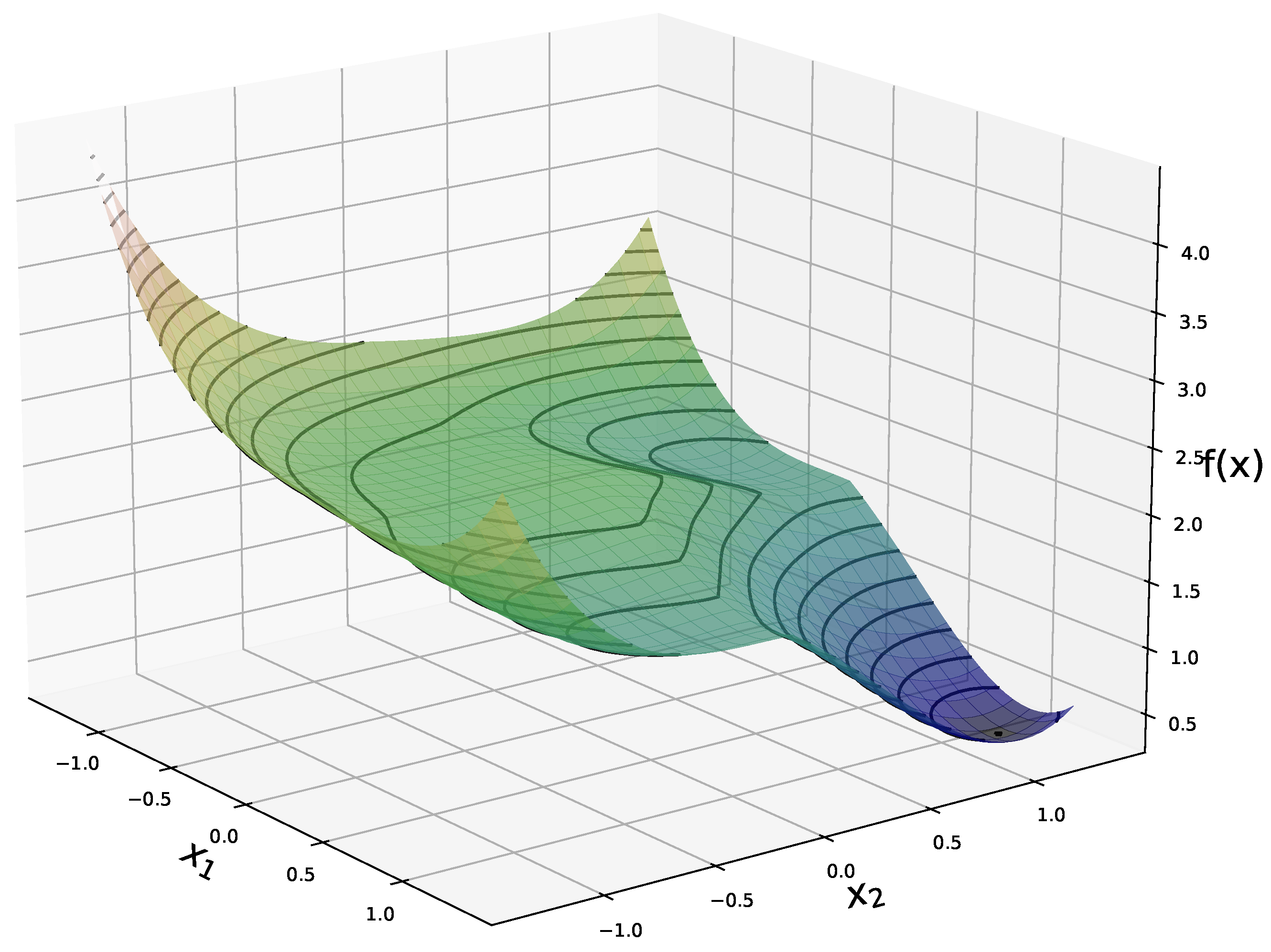
The reconstruction method presented in Algorithm 1 is motivated by the landscape analysis of the minimization problem (4) for a network G with sufficiently-expansive Gaussian weights matrices. Under this assumption, we showed in [31] that (4) has a benign optimization geometry and in particular that for any nonzero point outside a neighborhood of $x_{🟉}$ and a negative multiple of it, any subgradient of f is a direction of strict descent. Furthermore we showed that the points in the vicinity of the spurious negative multiple of $x_{🟉}$ have function values strictly larger than those close to $x_{🟉}$. Figure 1 shows the expected value of f in the noiseless case, $\nu =0$ and $N\to \infty$, for a generative network with latent dimension $k=2$. This plot highlights the global minimimum at $x_{🟉}=[1,1]$, and the flat region in near a negative multiple of $x_{🟉}$.

At each step, the subgradient method in Algorithm 1 checks if the current iterate $x_i$ has a larger loss value than its negative multiple, and if so negates $x_i$. As we show in the proof of our main result, this step will ensure that the algorithm will avoid the neighborhood around the spurious negative multiple of $x_{🟉}$ and will converge to the neighborhood around $x_{🟉}$ in a polynomial number of steps.

Below we make the following assumptions on the weight matrices of G.

Assumption 1.

The generative network G defined in (3), has weights $W_i\in {\mathbb{R}}^{n_i\times n_{i-1}}$ with i.i.d. entries from $\mathcal{N}(0,1/n_i)$ and satisfying the expansivity condition with constant $ϵ>0$:

$$n_{i+1}\ge c{n}_i{ϵ}^{-2}\log (1/ϵ)$$

(10)

for all i and a universal constant $c>0$.

We note that in [31] the expansivity condition was more stringent, requiring an additional log factor. Since the publication of our paper, [62] has shown that the more relaxed assumption (10) suffices for ensuring a benign optimization geometry. Under Assumption 1, our main theorem below shows that the subgradient method in Algorithm 1 can estimate the spike $y_{🟉}$ with optimal sample complexity and in a polynomial number of steps.

Theorem 1.

Let $x_{🟉}\in {\mathbb{R}}^k$ nonzero and $y_{🟉}=G\left(x_{🟉}\right)$ where G is a generative network satisfying Assumption 1 with $ϵ\le K_1/d^{96}$. Consider the minimization problem (4) and assume that the noise level ω satisfies $\omega \le K_2{\Vert x_{🟉}\Vert }_2^2{2}^{-d}/d^{44}$ where:

• for theSpiked Wishart Model(1) take $M={\Sigma }_N-{\sigma }^2{I}_n$, and

  $$\omega :=(\Vert y_{🟉}{\Vert }_2^2+{\sigma }^2)\max \left\{\sqrt{\frac{338k\log (3n_1^d{n}_2^{d-1}\dots n_{d-1}^{2}n)}{N}},\frac{156k\log (3n_1^d{n}_2^{d-1}\dots n_{d-1}^{2}n)}{N}\right\};$$
• for theSpiked Wigner Model(2) take $M=Y$, and

  $$\omega :=\nu \sqrt{\frac{169k\log (3n_1^d{n}_2^{d-1}\dots n_{d-1}^{2}n)}{n}}.$$

Consider Algorithm 1 with nonzero $x_0$ and $\Vert x_0{\Vert }_2<R_{🟉}$ where $R_{🟉}\ge 5{\Vert x_{🟉}\Vert }_2/\left(2\sqrt{2}\right)$, and stepsize $\mu =2^{2d}{K}_3/(8d^4{R}_{🟉}^2)$. Then with probability at least $1-2e^{-k\log n}-{\sum }_{i=1}^d{e}^{-C{n}_{i-1}}$, $0<\Vert x_i{\Vert }_2<R_{🟉}$ for any $i\ge 1$, there exists an integer $T\le K_{4}f\left(x_0\right)2^{2d}/(R_{🟉}^4{d}^4ϵ)$ such that for any $i\ge T$:

$$\begin{array}{cc}\hfill \Vert x_{i+1}-x_{🟉}{\Vert }_2& \le {\mathsf{\rho }}_1^{i+1-T}{\Vert x_T-x_{🟉}\Vert }_2+{\mathsf{\rho }}_2\frac{2^d}{\Vert x_{🟉}{\Vert }_2}\omega \hfill \end{array}$$

(11)

$$\begin{array}{cc}\hfill \Vert G\left(x_{i+1}\right)-y_{🟉}{\Vert }_2& \le \frac{1.2}{2^{d/2}}{\mathsf{\rho }}_1^{i+1-T}{\Vert x_T-x_{🟉}\Vert }_2+1.3{\mathsf{\rho }}_2\frac{\omega }{\Vert y_{🟉}{\Vert }_2}\hfill \end{array}$$

(12)

where $C>0$, $K_1,\dots ,K_4>0$, ${\mathsf{\rho }}_1\in (0,1)$ and ${\mathsf{\rho }}_2>0$ are universal constants.

Note that the quantity $2^{2d}$ in the hypotheses and conclusions of the theorem is an artifact of the scaling of the network and it should not be taken as requiring exponentially small noise or number of steps. Indeed under Assumption 1, the ReLU activation zeros out roughly half of the entries of its argument leading to an “effective” operator norm of approximately $1/2$. We furthermore notice that the dependence of the depth d is likely quite conservative and it was not optimized in the proof as the main objective was to obtain tight dependence on the intrinsic dimension of the signal k. As shown in the numerical experiments, the actual dependence on the depth is much better in practice. Finally, observe that despite the nonconvex nature of the objective function in (4) we obtain a rate of convergence which is not directly dependent on the dimension of the signal, reminiscent of what happens in the convex case.

The quantity $\omega$ in Theorem 1 can be interpreted as the intrinsic noise level of the problem (inverse SNR). The theorem guarantees that in a polynomial number of steps the iterates of the subgradient method will converge to $x_{🟉}$ up to $\omega$. For $\tilde{T}$ large enough $G\left(x_{\tilde{T}}\right)$ will satisfy the rate-optimal error bounds (5) and (6).

Numerical Experiments

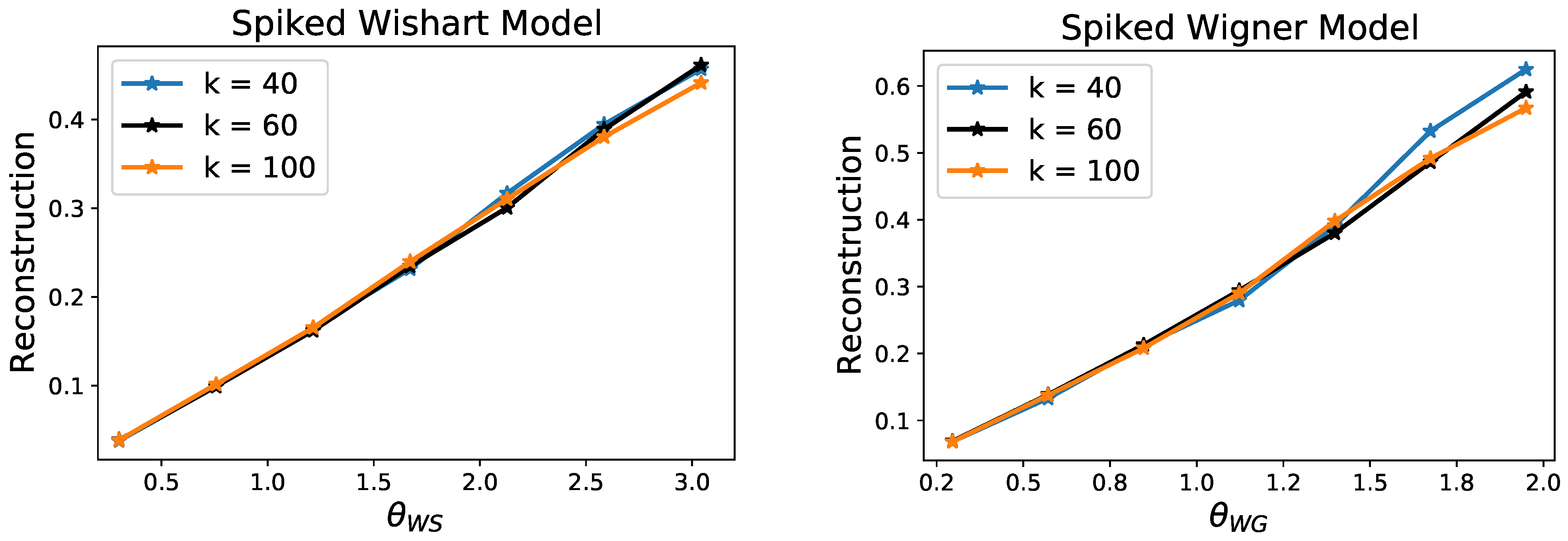
We illustrate the predictions of our theory by providing results of Algorithm 1 on a set of synthetic experiments. We consider 2-layer generative networks with ReLU activation functions, hidden layer of dimension $n_1=500$, output dimension $n_2=n=1500$ and varying number of latent dimension $k\in [40,60,100]$. We randomly sample the weights of the matrix independently from $\mathcal{N}(0,2/n_i)$ (this scaling removes that $2^d$ dependence in Theorem 1). We then consider data Y according the spiked models (1) and (2), where $x_{🟉}\in {\mathbb{R}}^k$ is chosen so that $y_{🟉}=G\left(x_{🟉}\right)$ has unit norm. For the Wishart model, we vary the number of samples N; and for the Wigner model, we vary the noise level $\nu$ so that the following quantities remain constant for the different networks with latent dimension k:

$${\theta }_{\mathrm{WS}}:=\sqrt{k\log \left(n_1^{2}n\right)/N},{\theta }_{\mathrm{WG}}:=\nu \sqrt{k\log \left(n_1^{2}n\right)/n}.$$

In Figure 2 we plot the reconstruction error given by $\Vert G\left(x\right)-y_{🟉}{\Vert }_2$ against ${\theta }_{\mathrm{WS}}$ and ${\theta }_{\mathrm{WG}}$. As predicted by Theorem 1, the errors scale linearly with respect to these control parameters, and moreover the overlap of these plots confirms that these rates are tight with respect to the order of k.

4. Recovery Under Deterministic Conditions

We will derive Theorem 1 from Theorem 3, below, which is based on a set of deterministic conditions on the weights of the matrix and the noise. Specifically, we consider the minimization problem (4) with

$$M=G\left(x_{🟉}\right)G{\left(x_{🟉}\right)}^{\mathsf{T}}+H$$

for an unknown symmetric matrix $H\in {\mathbb{R}}^{n\times n}$, nonzero $x_{🟉}\in {\mathbb{R}}^k$, and a given d-layer feed forward generative network G as in (3).

In order to describe the main deterministic conditions on the generative network G, we begin by introducing some notation. For $W\in {\mathbb{R}}^{n\times k}$ and $x\in {\mathbb{R}}^k$, we define the operator $W_{+,x}:=\mathrm{diag}(Wx>0)W$ such that $\mathrm{relu}\left(Wx\right)=W_{+,x}x$. Moreover, we let $W_{1,+,x}={\left(W_1\right)}_{+,x}=\mathrm{diag}(W_{1}x>0)W_1$, and for $2\le i\le d$ we define recursively

$$W_{i,+,x}=\mathrm{diag}(W_i,{\Pi }_{j=i-1}^1{W}_{j,+,x}x>0)W_i,$$

where ${\Pi }_{i=d}^1{W}_i=W_d{W}_{d-1}\dots W_1$. Finally we let ${\Lambda }_x={\Pi }_{j=d}^1{W}_{j,+,x}$ and note that $G\left(x\right)={\Lambda }_{x}x$. With this notation we next recall the following deterministic condition on the layers of the generative network.

Definition 2

(Weight Distribution Condition [15]). We say that $W\in {\mathbb{R}}^{n\times k}$ satisfies the Weight Distribution Condition (WDC) with constant $ϵ>0$ if for all nonzero $x_1,x_2\in {\mathbb{R}}^k$:

$$\Vert W_{+,x_1}^{\mathsf{T}}{W}_{+,x_2}-Q_{x_1,x_2}{\Vert }_2\le ϵ,$$

where

$$Q_{x_1,x_2}=\frac{\pi -{\theta }_{x_1,x_2}}{2\pi }{I}_k+\frac{\sin {\theta }_{x_1,x_2}}{2\pi }{M}_{{\widehat{x}}_2\leftrightarrow {\widehat{x}}_2}$$

and ${\theta }_{x_1,x_2}=\angle (x_1,x_2)$, ${\widehat{x}}_1=x_1/{\Vert x_1\Vert }_2$, ${\widehat{x}}_2=x_2/{\Vert x_2\Vert }_2$, $I_k$ is the $k\times k$ identity matrix and $M_{{\widehat{x}}_1\leftrightarrow {\widehat{x}}_2}$ is the matrix that sends ${\widehat{x}}_1\mapsto {\widehat{x}}_2$, ${\widehat{x}}_2\mapsto {\widehat{x}}_1$, and with kernel span ${\left(\{x_1,x_2\}\right)}^{\perp }$.

Note that $Q_{x_1,x_2}$ is the expected value of $W_{+,x_1}^{\mathsf{T}}{W}_{+,x_2}$ when W has rows $w_i\sim \mathcal{N}(0,I_k/n)$, and if $x_1=x_2$ then $Q_{x_1,y_2}$ is an isometry up to the scaling factor $1/2$. Below we will say that a d-layer generative network G of the form (3), satisfies the WDC with constant $ϵ>0$ if every weight matrix $W_i$ has the WDC with constant $ϵ$ for all $i=1,\dots d$.

The WDC was originally introduced in [15], and ensures that the angle between two vectors in the latent space is approximately preserved at the output layer and, in turn, it guarantees the invertibility of the network. Assumption 1 will guarantees that the generative network G satisfies the WDC with high probability.

We are now able to state our recovery guarantees for a spike $y_{🟉}$ under deterministic conditions on the network G and noise H.

Theorem 3.

Let $d\ge 2$ and assume the generative network (3) has weights $W_i\in {\mathbb{R}}^{n_i\times n_{i-1}}$ satisfying the WDC with constant $0<ϵ\le K_1/d^{96}$. Consider Algorithm 1 with $M=G\left(x_{🟉}\right)G{\left(x_{🟉}\right)}^{\mathsf{T}}+H$, $x_{🟉}\in {\mathbb{R}}^k\backslash \left\{0\right\}$ and H a symmetric matrix satisfying:

$$\parallel {\Lambda }_x^{\mathsf{T}}H{\Lambda }_x{\parallel }_2\le \frac{\omega }{2^d},\mathit{and}\omega \le K_2\frac{\parallel x_{🟉}{\parallel }_2^2{2}^{-d}}{d^{44}}.$$

(13)

Take $x_0$ nonzero and with $\Vert x_0{\Vert }_2<R_{🟉}$ where $R_{🟉}\ge 5{\Vert x_{🟉}\Vert }_2/\left(2\sqrt{2}\right)$, $\mu =2^{2d}{K}_3/(8d^4{R}_{🟉}^2)$. Then the iterates ${\left\{x_i\right\}}_{i\ge 0}$ generated by the Algorithm 1 satisfy $0<\Vert x_i\Vert <R_{🟉}$ and obey to the following:

(A) 

there exists an integer $T\le K_4\frac{f\left(x_0\right)2^{2d}}{R_{🟉}^4{d}^4ϵ}$ such that

$$\parallel x_T-x_{🟉}{\parallel }_2\le K_5{d}^{14}\sqrt{ϵ}\parallel x_{🟉}{\parallel }_2+K_6{2}^d{d}^{10}\omega {\parallel x_{🟉}\parallel }_2^{-1}$$

(B) 

for any $i\ge T$:

$$\begin{array}{cc}\hfill \parallel x_{i+1}-x_{🟉}{\parallel }_2& \le {\mathsf{\rho }}_1^{i+1-T}{\parallel x_T-x_{🟉}\parallel }_2+{\mathsf{\rho }}_2\frac{2^d}{\parallel x_{🟉}{\parallel }_2}\omega \hfill \end{array}$$

(14)

$$\begin{array}{cc}\hfill \Vert G\left(x_{i+1}\right)-G\left(x_{🟉}\right){\Vert }_2& \le \frac{1.2}{2^{d/2}}{\mathsf{\rho }}_1^{i+1-T}{\Vert x_T-x_{🟉}\Vert }_2+1.3{\mathsf{\rho }}_2\frac{\omega }{\Vert y_{🟉}{\Vert }_2}\hfill \end{array}$$

(15)

where $K_1,\dots ,K_6>0$, ${\mathsf{\rho }}_1\in (0,1)$ and ${\mathsf{\rho }}_2>0$ are universal constants.

Theorem 1 follows then from Theorem 3 after proving that with high probability the spectral norm of ${\Lambda }_x^{\mathsf{T}}H{\Lambda }_x$, where $H=M-y_{🟉}{y_{🟉}}^{\mathsf{T}}$, can be upper bounded by $\omega /2^d$, and the weights of the network G satisfy with high probability the WDC.

In the rest of this section section we will describe the main steps and tools needed to prove Theorem 3.

4.1. Technical Tools and Outline of the Proofs

Our proof strategy for Theorem 3 can be summarized as follows:

• In Proposition A1 (Appendix A.3) we show that the iterates ${\left\{x_i\right\}}_{i=1}$ of the Algorithm 1 stay inside the Euclidean ball of radius $R_{🟉}$ and remain nonzero for all $i\ge 1$.
• We then identify two small Euclidean balls ${\mathcal{B}}_{+}$ and ${\mathcal{B}}_{-}$ around respectively $x_{🟉}$ and $-{\rho }_d{x}_{🟉}$, where ${\rho }_d\in (0,1)$ only depends on the depth of the network. In Proposition A2 we show that after a polynomial number of steps, the iterates $\left\{x_i\right\}$ of the Algorithm 1 enter the region ${\mathcal{B}}_{+}\cup {\mathcal{B}}_{-}$ (Appendix A.4).
• We show, in Proposition A3, that the negation step causes the iterates of the algorithm to avoid the spurious point $-{\rho }_d{x}_{🟉}$ and actually enter ${\mathcal{B}}_{+}$ within a polynomial number of steps (Appendix A.5).
• We finally show in Proposition A4, that in ${\mathcal{B}}_{+}$ the loss function f enjoys a favorable convexity-like property, which implies that the iterates $\left\{x_i\right\}$ will remain in ${\mathcal{B}}_{+}$ and eventually converge to $x_{🟉}$ up to the noise level (Appendix A.6).

One of the main difficulties in the analysis of a subgradient method in Algorithm 1 is the lack of smoothness of the loss function f. We show that the WDC allows us to overcome this issue by showing that the subgradients of f are uniformly close, up to the noise level, to the vector field $h_x\in {\mathbb{R}}^k$:

$$h_x:=\frac{1}{2^{2d}}\left(x{x}^{\mathsf{T}}-{\tilde{h}}_x{\tilde{h}}_x^{\mathsf{T}}\right)x,$$

where ${\tilde{h}}_x$ is continuous for nonzero x (see Appendix A.2). We show furthermore that $h_x$ is locally Lipschitz, which allows us to conclude that the gradient method decreases the value of the loss function until eventually reaching ${\mathcal{B}}_{+}\cup {\mathcal{B}}_{-}$ (Appendix A.4).

Using the WDC, we show that the loss function f is uniformly close to

$$f_E\left(x\right)=\frac{1}{2^{2d+2}}\left({\Vert x\Vert }_2^4+{\Vert x_{🟉}\Vert }_2^4-2{\langle x,{\tilde{h}}_x\rangle }^2\right).$$

(16)

A direct analysis of $f_E$ reveals that its values inside ${\mathcal{B}}_{-}$ are strictly larger then those inside ${\mathcal{B}}_{+}$. This property extends to f as well, and guarantees that the gradient method will not converge to the spurious point $-{\rho }_d{x}_{🟉}$ (Appendix A.5).

References

- Johnstone, I.M. On the distribution of the largest eigenvalue in principal components analysis. Ann. Stat. 2001, 29, 295–327. [Google Scholar] [CrossRef]
- Amini, A.A.; Wainwright, M.J. High-dimensional analysis of semidefinite relaxations for sparse principal components. In Proceedings of the 2008 IEEE International Symposium on Information Theory, Toronto, ON, Canada, 6–11 July 2008; pp. 2454–2458. [Google Scholar]
- Deshpande, Y.; Montanari, A. Sparse PCA via covariance thresholding. In Proceedings of the Advances in Neural Information Processing Systems, Montréal, QC, Canada, 8–13 December 2014; pp. 334–342. [Google Scholar]
- Vu, V.; Lei, J. Minimax rates of estimation for sparse PCA in high dimensions. In Proceedings of the 15th International Conference on Artificial Intelligence and Statistics, La Palma, Canary Islands, Spain, 21–23 April 2012; pp. 1278–1286. [Google Scholar]
- Abbe, E.; Bandeira, A.S.; Bracher, A.; Singer, A. Decoding binary node labels from censored edge measurements: Phase transition and efficient recovery. IEEE Trans. Netw. Sci. Eng. 2014, 1, 10–22. [Google Scholar] [CrossRef] [Green Version]
- Bandeira, A.S.; Chen, Y.; Lederman, R.R.; Singer, A. Non-unique games over compact groups and orientation estimation in cryo-EM. Inverse Probl. 2020, 36, 064002. [Google Scholar] [CrossRef] [Green Version]
- Javanmard, A.; Montanari, A.; Ricci-Tersenghi, F. Phase transitions in semidefinite relaxations. Proc. Natl. Acad. Sci. USA 2016, 113, E2218–E2223. [Google Scholar] [CrossRef] [PubMed] [Green Version]
- McSherry, F. Spectral partitioning of random graphs. In Proceedings of the 42nd IEEE Symposium on Foundations of Computer Science, Newport Beach, CA, USA, 8–11 October 2001; pp. 529–537. [Google Scholar]
- Deshpande, Y.; Abbe, E.; Montanari, A. Asymptotic mutual information for the binary stochastic block model. In Proceedings of the 2016 IEEE International Symposium on Information Theory (ISIT), Barcelona, Spain, 10–15 July 2016; pp. 185–189. [Google Scholar]
- Moore, C. The computer science and physics of community detection: Landscapes, phase transitions, and hardness. arXiv 2017, arXiv:1702.00467. [Google Scholar]
- D’Aspremont, A.; Ghaoui, L.; Jordan, M.; Lanckriet, G. A direct formulation for sparse PCA using semidefinite programming. Adv. Neural Inf. Process. Syst. 2004, 17, 41–48. [Google Scholar] [CrossRef] [Green Version]
- Berthet, Q.; Rigollet, P. Optimal detection of sparse principal components in high dimension. Ann. Stat. 2013, 41, 1780–1815. [Google Scholar] [CrossRef] [Green Version]
- Bandeira, A.S.; Perry, A.; Wein, A.S. Notes on computational-to-statistical gaps: Predictions using statistical physics. arXiv 2018, arXiv:1803.11132. [Google Scholar] [CrossRef] [Green Version]
- Kunisky, D.; Wein, A.S.; Bandeira, A.S. Notes on computational hardness of hypothesis testing: Predictions using the low-degree likelihood ratio. arXiv 2019, arXiv:1907.11636. [Google Scholar]
- Hand, P.; Voroninski, V. Global guarantees for enforcing deep generative priors by empirical risk. IEEE Trans. Inf. Theory 2019, 66, 401–418. [Google Scholar] [CrossRef] [Green Version]
- Heckel, R.; Huang, W.; Hand, P.; Voroninski, V. Rate-optimal denoising with deep neural networks. arXiv 2018, arXiv:1805.08855. [Google Scholar]
- Hand, P.; Leong, O.; Voroninski, V. Phase retrieval under a generative prior. In Proceedings of the Advances in Neural Information Processing Systems, Montréal, QC, Canada, 3–8 December 2018; pp. 9136–9146. [Google Scholar]
- Ma, F.; Ayaz, U.; Karaman, S. Invertibility of convolutional generative networks from partial measurements. Adv. Neural Inf. Process. Syst. 2018, 31, 9628–9637. [Google Scholar]
- Hand, P.; Joshi, B. Global Guarantees for Blind Demodulation with Generative Priors. In Proceedings of the Advances in Neural Information Processing Systems, Vancouver, BC, Canada, 8–14 December 2019; pp. 11535–11543. [Google Scholar]
- Song, G.; Fan, Z.; Lafferty, J. Surfing: Iterative optimization over incrementally trained deep networks. In Proceedings of the Advances in Neural Information Processing Systems, Vancouver, BC, Canada, 8–14 December 2019; pp. 15034–15043. [Google Scholar]
- Bora, A.; Jalal, A.; Price, E.; Dimakis, A.G. Compressed sensing using generative models. In Proceedings of the 34th International Conference on Machine Learning, Sydney, Australia, 6–11 August 2017; Volume 70, pp. 537–546. [Google Scholar]
- Asim, M.; Shamshad, F.; Ahmed, A. Blind Image Deconvolution using Deep Generative Priors. arXiv 2019, arXiv:cs.CV/1802.04073. [Google Scholar] [CrossRef]
- Hand, P.; Leong, O.; Voroninski, V. Compressive Phase Retrieval: Optimal Sample Complexity with Deep Generative Priors. arXiv 2020, arXiv:2008.10579. [Google Scholar]
- Hand, P.; Voroninski, V. Compressed sensing from phaseless gaussian measurements via linear programming in the natural parameter space. arXiv 2016, arXiv:1611.05985. [Google Scholar]
- Li, X.; Voroninski, V. Sparse signal recovery from quadratic measurements via convex programming. SIAM J. Math. Anal. 2013, 45, 3019–3033. [Google Scholar] [CrossRef]
- Ohlsson, H.; Yang, A.Y.; Dong, R.; Sastry, S.S. Compressive phase retrieval from squared output measurements via semidefinite programming. arXiv 2011, arXiv:1111.6323. [Google Scholar] [CrossRef] [Green Version]
- Cai, T.; Li, X.; Ma, Z. Optimal rates of convergence for noisy sparse phase retrieval via thresholded Wirtinger flow. Ann. Stat. 2016, 44, 2221–2251. [Google Scholar] [CrossRef]
- Wang, G.; Zhang, L.; Giannakis, G.B.; Akçakaya, M.; Chen, J. Sparse phase retrieval via truncated amplitude flow. IEEE Trans. Signal Process. 2017, 66, 479–491. [Google Scholar] [CrossRef]
- Yuan, Z.; Wang, H.; Wang, Q. Phase retrieval via sparse wirtinger flow. J. Comput. Appl. Math. 2019, 355, 162–173. [Google Scholar] [CrossRef] [Green Version]
- Aubin, B.; Loureiro, B.; Maillard, A.; Krzakala, F.; Zdeborová, L. The spiked matrix model with generative priors. In Proceedings of the Advances in Neural Information Processing Systems, Vancouver, BC, Canada, 8–14 December 2019; pp. 8366–8377. [Google Scholar]
- Cocola, J.; Hand, P.; Voroninski, V. Nonasymptotic Guarantees for Spiked Matrix Recovery with Generative Priors. In Proceedings of the Advances in Neural Information Processing Systems, Vancouver, BC, Canada, 11 December 2020; Volume 33. [Google Scholar]
- Johnstone, I.M.; Lu, A.Y. On consistency and sparsity for principal components analysis in high dimensions. J. Am. Stat. Assoc. 2009, 104, 682–693. [Google Scholar] [CrossRef] [PubMed] [Green Version]
- Wainwright, M.J. High-Dimensional Statistics: A Non-Asymptotic Viewpoint; Cambridge University Press: Cambridge, UK, 2019; Volume 48. [Google Scholar]
- Montanari, A.; Richard, E. Non-negative principal component analysis: Message passing algorithms and sharp asymptotics. IEEE Trans. Inf. Theory 2015, 62, 1458–1484. [Google Scholar] [CrossRef] [Green Version]
- Deshpande, Y.; Montanari, A.; Richard, E. Cone-constrained principal component analysis. Adv. Neural Inf. Process. Syst. 2014, 27, 2717–2725. [Google Scholar]
- Zou, H.; Hastie, T.; Tibshirani, R. Sparse principal component analysis. J. Comput. Graph. Stat. 2006, 15, 265–286. [Google Scholar] [CrossRef] [Green Version]
- Krauthgamer, R.; Nadler, B.; Vilenchik, D.; others. Do semidefinite relaxations solve sparse PCA up to the information limit? Ann. Stat. 2015, 43, 1300–1322. [Google Scholar] [CrossRef]
- Berthet, Q.; Rigollet, P. Computational lower bounds for Sparse PCA. arXiv 2013, arXiv:1304.0828. [Google Scholar]
- Cai, T.; Ma, Z.; Wu, Y. Sparse PCA: Optimal rates and adaptive estimation. Ann. Stat. 2013, 41, 3074–3110. [Google Scholar] [CrossRef]
- Ma, T.; Wigderson, A. Sum-of-squares lower bounds for sparse PCA. Adv. Neural Inf. Process. Syst. 2015, 28, 1612–1620. [Google Scholar]
- Lesieur, T.; Krzakala, F.; Zdeborová, L. Phase transitions in sparse PCA. In Proceedings of the 2015 IEEE International Symposium on Information Theory (ISIT), Hong Kong, China, 14–19 June 2015; pp. 1635–1639. [Google Scholar]
- Brennan, M.; Bresler, G. Optimal average-case reductions to sparse pca: From weak assumptions to strong hardness. arXiv 2019, arXiv:1902.07380. [Google Scholar]
- Arous, G.B.; Wein, A.S.; Zadik, I. Free energy wells and overlap gap property in sparse PCA. In Proceedings of the Conference on Learning Theory, PMLR, Graz, Austria, 9–12 July 2020; pp. 479–482. [Google Scholar]
- Fan, J.; Liu, H.; Wang, Z.; Yang, Z. Curse of heterogeneity: Computational barriers in sparse mixture models and phase retrieval. arXiv 2018, arXiv:1808.06996. [Google Scholar]
- Richard, E.; Montanari, A. A statistical model for tensor PCA. Adv. Neural Inf. Process. Syst. 2014, 27, 2897–2905. [Google Scholar]
- Decelle, A.; Krzakala, F.; Moore, C.; Zdeborová, L. Asymptotic analysis of the stochastic block model for modular networks and its algorithmic applications. Phys. Rev. E 2011, 84, 066106. [Google Scholar] [CrossRef] [PubMed] [Green Version]
- Perry, A.; Wein, A.S.; Bandeira, A.S.; Moitra, A. Message-Passing Algorithms for Synchronization Problems over Compact Groups. Commun. Pure Appl. Math. 2018, 71, 2275–2322. [Google Scholar] [CrossRef] [Green Version]
- Oymak, S.; Jalali, A.; Fazel, M.; Eldar, Y.C.; Hassibi, B. Simultaneously structured models with application to sparse and low-rank matrices. IEEE Trans. Inf. Theory 2015, 61, 2886–2908. [Google Scholar] [CrossRef] [Green Version]
- Dhar, M.; Grover, A.; Ermon, S. Modeling sparse deviations for compressed sensing using generative models. arXiv 2018, arXiv:1807.01442. [Google Scholar]
- Shah, V.; Hegde, C. Solving linear inverse problems using gan priors: An algorithm with provable guarantees. In Proceedings of the 2018 IEEE International Conference on Acoustics, Speech and Signal Processing (ICASSP), Calgary, AB, Canada, 15–20 April 2018; pp. 4609–4613. [Google Scholar]
- Mixon, D.G.; Villar, S. Sunlayer: Stable denoising with generative networks. arXiv 2018, arXiv:1803.09319. [Google Scholar]
- Yeh, R.A.; Chen, C.; Lim, T.Y.; Schwing, A.G.; Hasegawa-Johnson, M.; Do, M.N. Semantic image inpainting with deep generative models. arXiv 2016, arXiv:1607.07539. [Google Scholar]
- Sønderby, C.K.; Caballero, J.; Theis, L.; Shi, W.; Huszár, F. Amortised map inference for image super-resolution. arXiv 2016, arXiv:1610.04490. [Google Scholar]
- Yang, G.; Yu, S.; Dong, H.; Slabaugh, G.; Dragotti, P.L.; Ye, X.; Liu, F.; Arridge, S.; Keegan, J.; Guo, Y.; et al. DAGAN: Deep de-aliasing generative adversarial networks for fast compressed sensing MRI reconstruction. IEEE Trans. Med. Imaging 2017, 37, 1310–1321. [Google Scholar] [CrossRef] [Green Version]
- Qiu, S.; Wei, X.; Yang, Z. Robust One-Bit Recovery via ReLU Generative Networks: Improved Statistical Rates and Global Landscape Analysis. arXiv 2019, arXiv:1908.05368. [Google Scholar]
- Xue, Y.; Xu, T.; Zhang, H.; Long, L.R.; Huang, X. Segan: Adversarial network with multi-scale l 1 loss for medical image segmentation. Neuroinformatics 2018, 16, 383–392. [Google Scholar] [CrossRef] [PubMed] [Green Version]
- Heckel, R.; Hand, P. Deep Decoder: Concise Image Representations from Untrained Non-convolutional Networks. In Proceedings of the International Conference on Learning Representations, New Orleans, LA, USA, 6–9 May 2019. [Google Scholar]
- Heckel, R.; Soltanolkotabi, M. Denoising and regularization via exploiting the structural bias of convolutional generators. arXiv 2019, arXiv:1910.14634. [Google Scholar]
- Heckel, R.; Soltanolkotabi, M. Compressive sensing with un-trained neural networks: Gradient descent finds the smoothest approximation. arXiv 2020, arXiv:2005.03991. [Google Scholar]
- Aubin, B.; Loureiro, B.; Baker, A.; Krzakala, F.; Zdeborová, L. Exact asymptotics for phase retrieval and compressed sensing with random generative priors. In Proceedings of the First Mathematical and Scientific Machine Learning Conference, PMLR, Princeton, NJ, USA, 20–24 July 2020; pp. 55–73. [Google Scholar]
- Clason, C. Nonsmooth Analysis and Optimization. arXiv 2017, arXiv:1708.04180. [Google Scholar]
- Daskalakis, C.; Rohatgi, D.; Zampetakis, M. Constant-Expansion Suffices for Compressed Sensing with Generative Priors. arXiv 2020, arXiv:2006.04237. [Google Scholar]
- Chi, Y.; Lu, Y.M.; Chen, Y. Nonconvex optimization meets low-rank matrix factorization: An overview. IEEE Trans. Signal Process. 2019, 67, 5239–5269. [Google Scholar] [CrossRef] [Green Version]
- Vershynin, R. High-Dimensional Probability: An Introduction with Applications in Data Science; Cambridge University Press: Cambridge, UK, 2018; Volume 47. [Google Scholar]
Figure 1.
Expected value, with respect to the weights, of the objective function f in (4) in the noiseless case (see (16) for explicit formula), for a network with latent dimension and .
Figure 2.
Reconstruction error for the recovery of a spike in the Wishart and Wigner models with random generative network priors. Each point corresponds to the average over 50 random drawing of the network weights and samples. These plots demonstrate that the reconstruction errors follow the scalings established by Theorem 1.
Publisher’s Note: MDPI stays neutral with regard to jurisdictional claims in published maps and institutional affiliations. |
© 2021 by the authors. Licensee MDPI, Basel, Switzerland. This article is an open access article distributed under the terms and conditions of the Creative Commons Attribution (CC BY) license (http://creativecommons.org/licenses/by/4.0/).
Share and Cite
MDPI and ACS Style
Cocola, J.; Hand, P.; Voroninski, V. No Statistical-Computational Gap in Spiked Matrix Models with Generative Network Priors. Entropy 2021, 23, 115. https://doi.org/10.3390/e23010115
AMA Style
Cocola J, Hand P, Voroninski V. No Statistical-Computational Gap in Spiked Matrix Models with Generative Network Priors. Entropy. 2021; 23(1):115. https://doi.org/10.3390/e23010115
Chicago/Turabian StyleCocola, Jorio, Paul Hand, and Vladislav Voroninski. 2021. "No Statistical-Computational Gap in Spiked Matrix Models with Generative Network Priors" Entropy 23, no. 1: 115. https://doi.org/10.3390/e23010115
Note that from the first issue of 2016, this journal uses article numbers instead of page numbers. See further details here.