Prospectivity Mapping for Magmatic-Related Seafloor Massive Sulfide on the Mid-Atlantic Ridge Applying Weights-of-Evidence Method Based on GIS

Abstract

The Mid-Atlantic Ridge belongs to slow-spreading ridges. Hannington predicted that there were a large number of mineral resources on slow-spreading ridges; however, seafloor massive sulfide deposits usually develop thousands of meters below the seafloor, which make them extremely difficult to explore. Therefore, it is necessary to use mineral prospectivity mapping to narrow the exploration scope and improve exploration efficiency. Recently, Fang and Shao conducted mineral prospectivity mapping of seafloor massive sulfide on the northern Mid-Atlantic Ridge, but the mineral prospectivity mapping of magmatic-related seafloor massive sulfide on the whole Mid-Atlantic Ridge scale has not yet been carried out. In this study, 11 types of data on magmatic-related seafloor massive sulfide mineralization were collected on the Mid-Atlantic Ridge, namely water depth, slope, oceanic crust thickness, large faults, small faults, ridge, bedrock age, spreading rate, Bouguer gravity, and magnetic and seismic point density. Then, the favorable information was extracted from these data to establish 11 predictive maps and to create a mineral potential model. Finally, the weights-of-evidence method was applied to conduct mineral prospectivity mapping. Weight values indicate that oceanic crust thickness, large faults, and spreading rate are the most important prospecting criteria in the study area, which correspond with important ore-controlling factors of magmatic-related seafloor massive sulfide on slow-spreading ridges. This illustrates that the Mid-Atlantic Ridge is a typical slow-spreading ridge, and the mineral potential model presented in this study can also be used on other typical slow-spreading ridges. Seven zones with high posterior probabilities but without known hydrothermal fields were delineated as prospecting targets. The results are helpful for narrowing the exploration scope on the Mid-Atlantic Ridge and can guide the investigation of seafloor massive sulfide resources efficiently.

1. Introduction

Due to increasing demand, mineral resources on land are depleting. However, the progress of deep-sea exploration techniques has made exploration of seafloor mineral resources a popular research subject [1]. Seafloor massive sulfides have attracted attention because of their rich copper, zinc, gold, and silver contents [2]. The process of seafloor massive sulfide mineralization is similar to that of ancient volcanic massive sulfide deposits preserved on land, both of which are formed by hydrothermal fluid. Since the first hydrothermal field was discovered on the Galapagos Rift in 1977, the number of hydrothermal fields discovered has steadily increased [3]. More than 700 hydrothermal fields have been discovered [4], approximately 86% of which are located on mid-ocean ridges, and 76 hydrothermal fields are located on the Mid-Atlantic Ridge (InterRidge Vents Database). However, the exploration of seafloor massive sulfide resources is still relatively new [5]. As seafloor massive sulfide deposits develop in the seafloor, delineating the prospecting targets quickly and accurately is essential.

In the 21st century, the development of big data has provided a new way to quantitatively predict the locations of seafloor massive sulfides. Compared with mineral resources on land, due to the limitations of physical conditions and techniques, very little exploration has been done on seafloor massive sulfides; therefore, data related to their mineralization are limited. In this study, using big data methods, we extracted favorable information from available data to obtain prediction maps and transformed the conceptual model into a quantitative mineral potential model. Recently, Fang and Shao conducted two and three dimensional mineral prospectivity mapping of the northern Mid-Atlantic Ridge [6,7]. The above results can provide a basis for reducing the exploration scope; however, the mineral prospectivity mapping of magmatic-related seafloor massive sulfides has not been conducted for the entire Mid-Atlantic Ridge.

We collected 11 types of data covering the Mid-Atlantic Ridge, namely water depth, slope, oceanic crust thickness, large faults, small faults, mid-ocean ridge, bedrock age, spreading rate, Bouguer gravity, magnetism, and seismic point density, and present a quantitative mineral potential model for magmatic-related seafloor massive sulfide on the Mid-Atlantic Ridge. Based on the quantitative mineral potential model, the weights-of-evidence method was applied for mineral prospectivity mapping. By comparing prediction maps with high weight values in the study area to important ore-forming factors on slow-spreading ridges, we determined that the Mid-Atlantic Ridge is a typical slow-spreading ridge. Therefore, the mineral potential model in this study can also be used in other typical slow-spreading ridges. In addition, 7 prospecting targets with high posterior probabilities were delineated, which provide a basis for the exploration of magmatic-related seafloor massive sulfides on the Mid-Atlantic Ridge.

2. Study Area

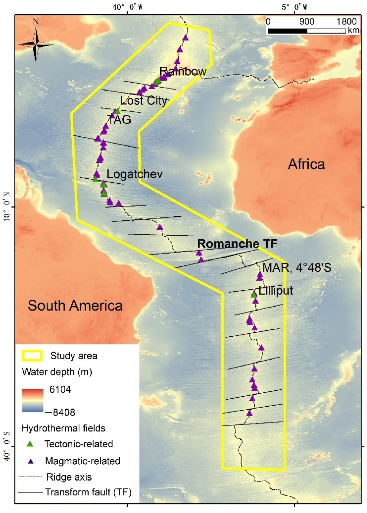
The Mid-Atlantic Ridge extends across the middle of the Atlantic Ocean in an inverse ‘T’ shape. It is a slow-spreading ridge, stretching from 87° N to 54° S [8]. The average width of the Mid-Atlantic Ridge is approximately 1000–1300 km, and the length is 17,000 km, accounting for 40% of the total length of global mid-ocean ridges. Along the central axis of the Mid-Atlantic Ridge, there is a longitudinal rift valley 15–30 km wide and approximately 2 km deep, splitting the ridge in the middle, and the valley floor is approximately 1800 m lower than the peak [9]. Tectonic activities surrounding the Mid-Atlantic Ridge are intense. A highly developed transverse transform fault cuts the ridge into several segments. In some areas, such as the Logatchev hydrothermal field, there are large detachment faults, that when combined with extensive tectonic activities, result in the exposure of rocks from the lower crust (gabbro) and upper mantle (peridotite).

Bounded by the Romanche transform fault near the equator, the Atlantic can be divided into the north Atlantic and south Atlantic. The northern Mid-Atlantic Ridge at 5.9–65.8° N is one of the most studied mid-ocean ridges for hydrothermal activities, where seafloor massive sulfide deposits primarily occur, and the deposits are uniformly distributed with an average distance of approximately 78 km. Famous hydrothermal fields such as TAG, Logatchev, Rainbow, and Lost City have been discovered on the northern Mid-Atlantic Ridge. A survey of hydrothermal activities on the southern Mid-Atlantic Ridge was started in 2005, where several hydrothermal fields have been found, including Red Lion, Turtle Pits, Wideawake, and Lilliput (Figure 1).

3. Genesis of Seafloor Massive Sulfide Deposits on the Mid-Atlantic Ridge

On mid-ocean ridges, seafloor massive sulfides form through the following process: First, cold seawater flows into a channel formed by fissures in the oceanic crust or rock fractures. In this process, cold seawater is heated by heat sources such as magma, and metallic elements such as Cu, Fe, Zn, and Pb in the wall rock are leached out. Subsequently, the heated seawater rises from the channel, forming hydrothermal sediments in vents, which is considered the seafloor massive sulfide. Studies of modern seafloor massive sulfide deposits show that the seafloor massive sulfide mineralization is controlled by various factors, including deep magmatic activities, faults, seafloor topography, spreading rate, sediment, and the type and permeability of wall rocks. Mineralization outcrops, tectonism, geomorphologic shape, hydrothermal plumes, and geophysical and geochemical information are prospecting indicators for seafloor massive sulfide. Compared with the amount of seafloor massive sulfide formed on fast-spreading ridges, the number of deposits formed on the Mid-Atlantic Ridge is higher due to its high permeability caused by intense tectonic activities, large numbers of channels created by detachment faults, and a stable metallogenic environment [10]. According to the genesis of seafloor massive sulfide deposits, the hydrothermal fields on the Mid-Atlantic Ridge can be defined as either magmatic-related or tectonic-related.

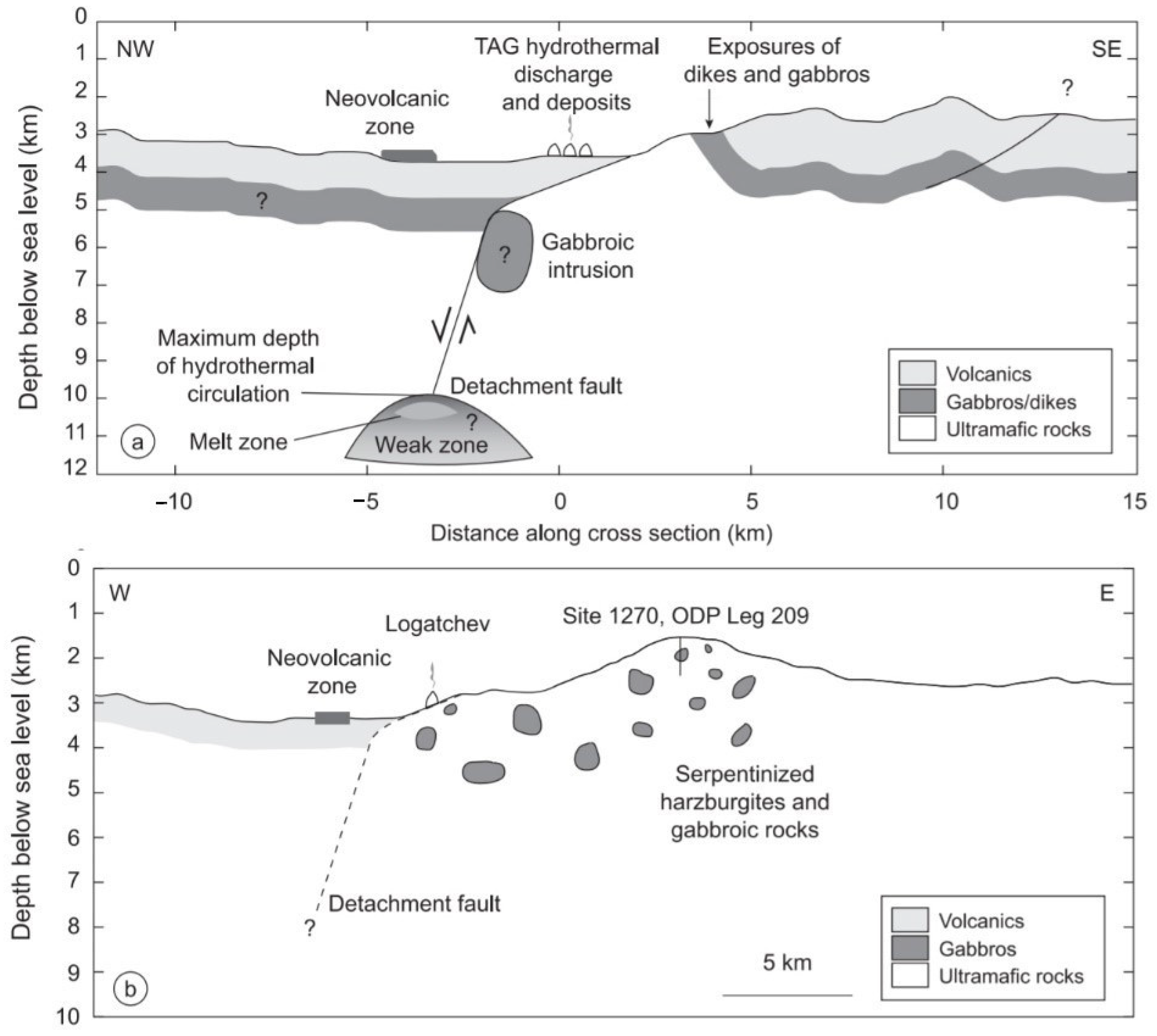
Magmatic-related hydrothermal fields are formed in mafic volcanic rocks, including mid-oceanic ridge basalt and gabbro. The water depth of seafloor massive sulfide mineralization varies widely, from 1500 to 5000 m. The available metallic elements are primarily Cu and Zn, but the amounts of Cu and Zn in seafloor massive sulfides in magmatic-related hydrothermal fields are less than those in tectonic hydrothermal fields. There are 76 magmatic-related hydrothermal fields on the Mid-Atlantic Ridge, including TAG, Lucky Strike, and Broken Spur, among which TAG is the largest [11]. The TAG hydrothermal field was formed near the hanging wall of the detachment fault (Figure 2a). The basement rocks are primarily basalts in the upper oceanic crust, and the metallogenic materials tend to originate from the basalts. The heat source driving the hydrothermal circulation does not come from the new volcanic center at the axis, but is related to the gabbro intrusion [12]. Owing to the poor permeability of massive or pillow volcanic rocks, the hydrothermal fluid can only be discharged in an aggregate form along major faults. At the same time, the stability of the hydrothermal system and the superposition of multiple hydrothermal events result in the accumulation of seafloor massive sulfides in a small area on the seafloor.

The basement of tectonic-related hydrothermal fields is comprised of ultramafic abyssal peridotites. This type of hydrothermal field often develops in the rift valley wall at the end of the amagmatic segment on mid-ocean ridges (such as Logatchev 1 and Logatchev 2) (Figure 2b), in transform faults between segments (such as Lost City), and in non-transform discontinuities (such as Rainbow) [13]. Their mineralization is primarily controlled by tectonic activities related to detachment faults and gabbro intrusion. Detachment faults provide a heat source and channels for tectonic-related seafloor massive sulfide mineralization [12,14]. When the source of heat is deep below the seafloor, detachment faults can cause the hydrothermal fluid to migrate up to ten km along the channel, resulting in the formation of seafloor massive sulfide far away from the heat source [15]. For example, Logatchev 2 is 12 km off the ridge axis, and Lost City is 15 km off the axis. The geological setting of Lost City greatly extends the possible location of hydrothermal fields controlled by detachment faults on slow-spreading ridges rather than around the axis of mid-ocean ridges. When gabbro intrusions control tectonic-related seafloor massive sulfide mineralization, the heat comes not only from mantle material cooling and serpentinization but also from geothermal gradient warming and deep lithospheric heat on mid-ocean ridges [16].

4. Data Compilation, Mapping, and Mineral Potential Model

When establishing predictive maps for the model, we should extract a favorable interval containing the most training data in the smallest area [18]. By spatial analysis of known hydrothermal fields and collected data, the corresponding favorable intervals were obtained. According to these intervals, we delineated 11 predictive maps and then combined them to form a mineral potential model.

4.1. Data Compilation and Mapping

4.1.1. Hydrothermal Fields

We used 65 magmatic-related hydrothermal fields on the Mid-Atlantic Ridge as training data in mineral prospectivity mapping, including 52 active hydrothermal fields and 13 inactive hydrothermal fields. These data were obtained from InterRidge Vents Database 3.4 and published papers (

Table 1. Basic information about hydrothermal fields.

ID	Name	Longitude	Latitude	Activity
1	AMAR	−33.65	36.38	active, inferred
2	Ashadze 4	−44.85	12.97	inactive
3	Broken Spur	−43.17	29.17	active, confirmed
4	Bubbylon	−31.53	37.80	active, confirmed
5	Deyin-1	−13.36	−15.17	active, confirmed
6	Evan	−32.28	37.27	active, confirmed
7	Krasnov	−46.48	16.64	inactive
8	Lilliput	−13.18	−9.55	active, confirmed
9	Logatchev 3	−44.97	14.71	active, inferred
10	Logatchev 4	−44.91	14.71	inactive
11	Lucky Strike	−32.27	37.29	active, confirmed
12	Sth. Lucky Strike, NTO3	−32.42	37.05	active, inferred
13	Luso	−29.88	38.98	active, confirmed
14	MAR, 11 26′ N	−43.70	11.45	active, inferred
15	MAR, 11 N	−43.65	11.04	active, inferred
16	MAR, 12 48′ N	−44.79	12.80	inactive
17	MAR, 13 19′N OCC	−44.90	13.33	active, inferred
18	MAR, 14 54′ N	−44.90	14.92	active, inferred
19	MAR, 16 46′ N	−46.38	16.80	inactive
20	MAR, 17 09′ N	−46.42	17.15	active, inferred
21	MAR, 19 S	−11.94	−19.33	active, inferred
22	MAR, 22 30′ N	−45.01	22.50	inactive
23	MAR, 23 35′ N	−45.00	23.58	inactive
24	MAR, 23 S	−13.39	−23.74	active, inferred
25	MAR, 24 20 ′N	−46.20	24.35	inactive
26	MAR, 24 30′ N	−46.15	24.50	inactive
27	MAR, 25 50′ N	−44.98	25.81	inactive
28	MAR, 27 N	−44.50	27.00	active, inferred
29	MAR, 27 S	−13.48	−27.15	active, inferred
30	MAR, 28 S	−13.37	−27.79	active, inferred
31	MAR, 30 N	−42.50	30.03	active, inferred
32	MAR, 30 S	−13.85	−29.95	active, inferred
33	MAR, 33 S	−14.44	−33.02	active, inferred
34	MAR, 4 02′ S	−12.25	−4.03	active, inferred
35	MAR, 4 48′ S	−12.37	−4.81	active, confirmed
36	MAR, 43 N	−29.00	43.00	active, inferred
37	MAR, 7 57′ S	−13.44	−7.95	active, inferred
38	MAR, 8 10′ S	−13.47	−8.17	active, inferred
39	MAR, segment south of St. Paul system	−25.00	0.50	active, inferred
40	MAR, south of 15 20′ N fracture zone	−45.00	15.08	active, inferred
41	Markov Deep	−33.18	5.91	active, inferred
42	Menez Gwen	−31.53	37.84	active, confirmed
43	Menez Hom	−32.43	37.15	active, confirmed
44	Merian	−13.85	−26.02	active, inferred
45	Moytirra	−27.85	45.48	active, confirmed
46	N Oceanographer	−34.87	35.28	active, inferred
47	Neptune′s Beard	−44.90	12.91	active, inferred
48	North FAMOUS	−32.97	36.97	active, inferred
49	Puy des Folles	−45.64	20.51	active, inferred
50	Rainbow Bay	−14.34	−14.03	active, inferred
51	Romanche Fracture Zone	−24.51	−0.98	inactive
52	S AMAR 1	−34.08	36.08	active, inferred
53	S AMAR 2	−34.18	35.97	active, inferred
54	S Oceanographer	−36.43	34.87	active, inferred
55	S-OH1	−36.85	34.53	active, inferred
56	S-OH2	−37.48	34.07	active, inferred
57	Semyenov	−44.96	13.51	active, confirmed
58	Snake Pit	−44.95	23.37	active, confirmed
59	South Kurchatov	−29.55	40.47	active, inferred
60	St. Petersburg	−45.87	19.87	active, inferred
61	TAG	−44.83	26.14	active, confirmed
62	TaiJi	−14.52	−13.59	active, inferred
63	Vema Fracture Zone	−41.80	10.85	inactive
64	Zenith-Victory	−45.62	20.13	inactive
65	Zouyu ridge	−14.41	−13.28	active, confirmed

) [13,19].

4.1.2. Terrain Information

Water Depth

The main influence of water depth on seafloor massive sulfide deposits is its control of the boiling of fluid and vapor phase separation. The greater the water depth and pressure, the higher the boiling point of the corresponding fluid. If a fluid is less likely to boil, the seafloor massive sulfide rapidly deposits and is metallogenic. The temperature of a hydrothermal fluid on the modern seafloor is generally around 350 °C. This temperature is exactly the boiling point corresponding to the pressure at a water depth of 1500 m [10]. Therefore, 1500 m is the critical depth condition for the formation of large seafloor massive sulfide deposits [20]. When the water depth is less than 1500 m, such as in the Menez Gwen hydrothermal field, which is 800 m deep, the boiling point and metal content of the hydrothermal fluid decrease. In that case, the formation of seafloor massive sulfide deposits is inhibited.

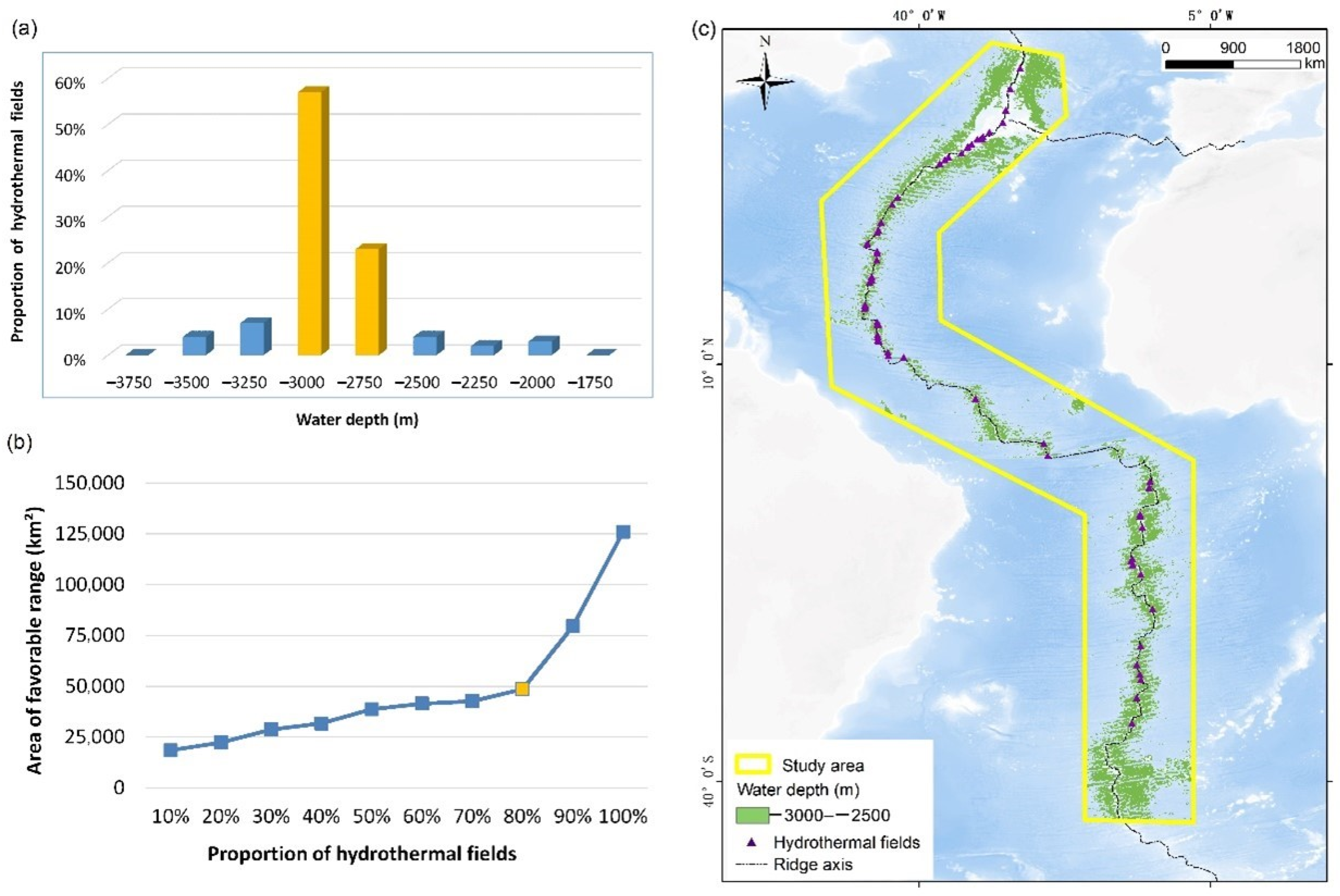
Water depth data were obtained from the ETOPO1 model of the National Oceanic and Atmospheric Administration (NOAA) Geophysical Data Center (NGDC), which integrates land topography and ocean bathymetry at a resolution of 1 × 1′ [21]. Water depth statistics where magmatic-related hydrothermal fields developed in the study area suggest that 80% of the magmatic-related hydrothermal fields occurred in areas with water depths ranging from 3000 to 2500 m below the ocean surface (Figure 3a). This interval covers 48618 km² in the study area. When the range increases, more hydrothermal fields will be covered. However, the area corresponding to this range will also rise dramatically, which contrasts to the principle that the most training data should locate in the smallest area (Figure 3b). Therefore, −3000 to −2500 m can be used as the favorable water depth interval in the predictive map (Figure 3c).

Slope Gradient

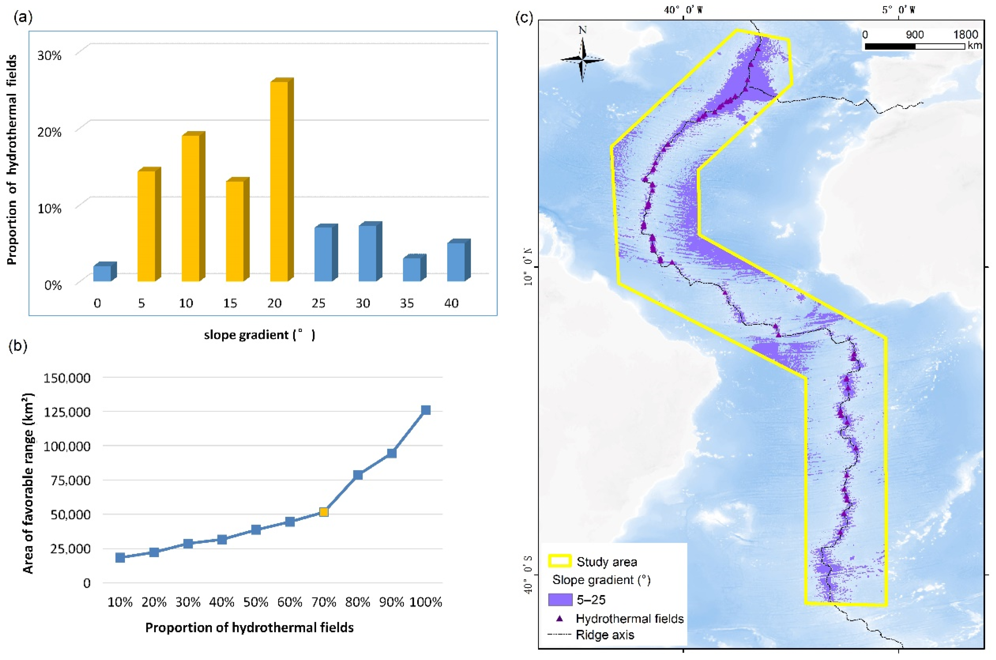
The slope gradient can reflect the topographic and geomorphic features of the seafloor. On mid-ocean ridges, most hydrothermal fields appear in the low-lying part of a high terrain, while a few appear in the higher part of a low terrain. This means that hydrothermal fields are not usually found at the top of mid-ocean ridges, but on graben at the ridge axis, volcanic highlands of rift valleys, slopes of ridge flanks, and tops of rift valley walls. For example, the Snake Pit, Lucky Strike, and Broken Spur hydrothermal fields developed on the volcanic highlands of rift valleys [13], and TAG and Krasnov hydrothermal fields are on the top of rift valley walls [22]. Using the surface analysis function of ArcGIS, we obtained the slope gradient from water depth data. The slope at the flanks on the Mid-Atlantic Ridge is steep due to its slow spreading rate. Statistics of the slope gradient where magmatic-related hydrothermal fields developed in the study area suggest that 72% of magmatic-related hydrothermal fields occurred in areas with slope gradients from 5° to 25° (Figure 4a). This interval covers 51,613 km² in the study area. When the range increases, more hydrothermal fields will be covered. However, the area corresponding to this range will also rise dramatically, which contrasts to the principle that the most training data should locate in the smallest area (Figure 4b). Therefore, the range from 5° to 25° can be used as the favorable interval in the predictive map of the slope gradient (Figure 4c).

4.1.3. Geological Information

Oceanic Crust Thickness

The oceanic crust thickness reflects the magma supply and magmatic process on mid-oceanic ridges. The thicker the oceanic crust, the greater the magma supply [23]. In the modern seafloor hydrothermal system, magmatic activities are sources of ore-forming materials and heat for seafloor massive sulfide deposits. It can be directly observed that quartz veins containing sulfide are closely related to gabbro intrusive bodies, and there are permeable sulfides in the gabbro in the deep 15°05′ N hydrothermal field on the Mid-Atlantic Ridge, which indicates that the ore-forming materials come from magmatic supply rather than the extraction from wall rocks. In addition, magmatic activity is the primary mechanism for releasing heat from the earth’s interior, about a third of which is released through the spreading center of ridges. Deep magma chambers transfer heat to seawater, creating a large-scale hydrothermal circulation system and leading to the formation of black chimneys on the seafloor [24]. This indicates that magmatic activities also provide a direct heat source for the formation of hydrothermal fields. The size of and available heat from the magma supply is dependent on various ridge spreading rates, which lead to the formation of the corresponding oceanic crust thickness [25].

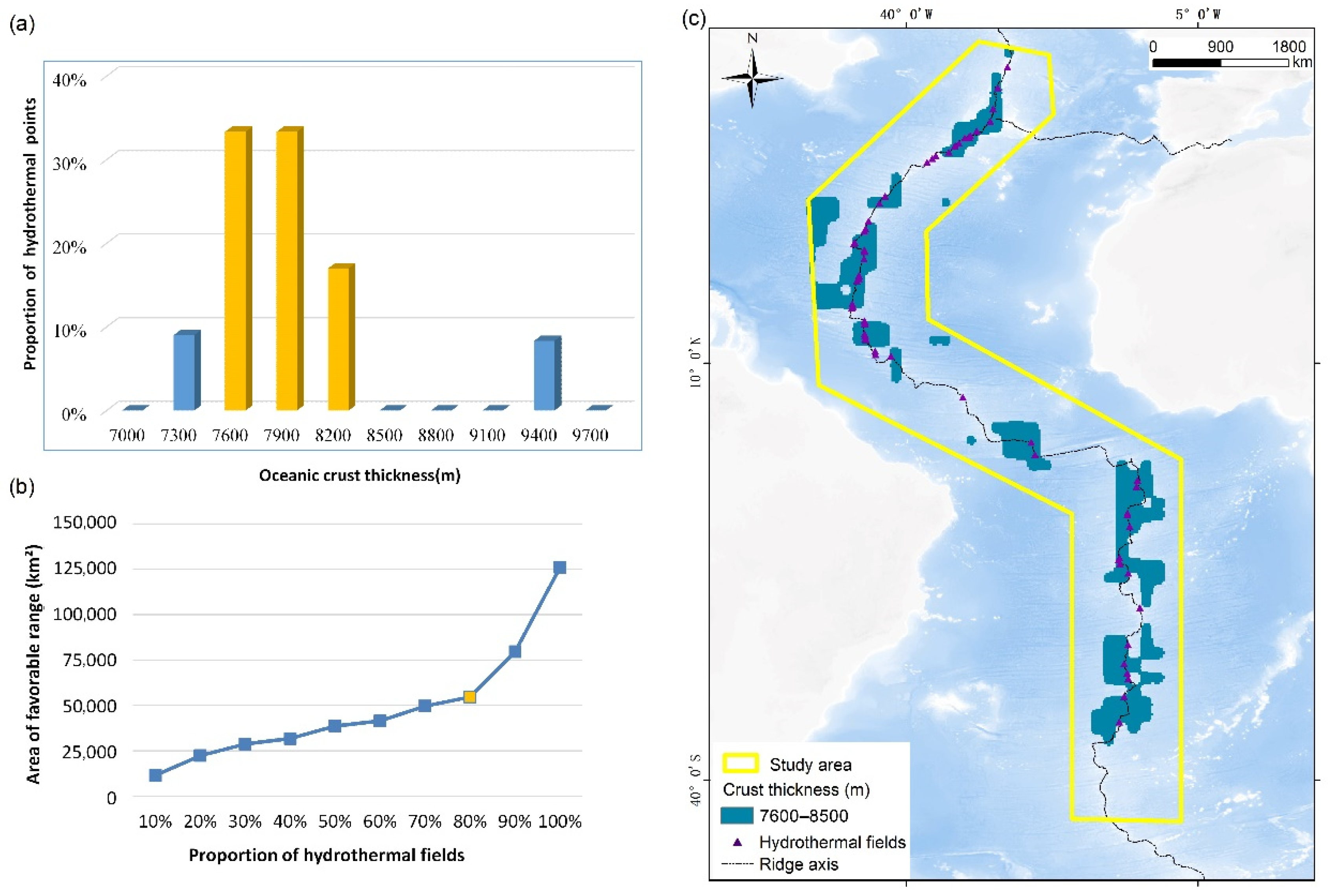
The oceanic crust thickness data are from a new global crustal model established by National Oceanic and Atmospheric Administration with a resolution of 5 × 5′. The oceanic crust on the Mid-Atlantic Ridge is relatively thin due to the lack of a magma chamber [26]. The structure of the oceanic crust is discontinuous along the ridge axis. The oceanic crust is relatively thick at the segment center, while it is relatively thin and lacks a transition fault and non-transform discontinuity at both ends of the ridge. Statistics of the oceanic crust thickness where magmatic-related hydrothermal fields developed in the study area suggest that 80% of magmatic-related hydrothermal fields occurred in areas with crust thicknesses ranging from 7600 to 8500 m (Figure 5a), which is a little thicker than the average oceanic crust thickness 6300 km on mid-ocean ridges [27]. It is because though the magma supply is low on the Mid-Atlantic Ridge, there are some ridge segments with high magma supply and the according oceanic crust thickness is thick. Hydrothermal massive sulfides often form there. This interval from 7600 to 8500 m covers 54,618 km² in the study area. When the range increases, more hydrothermal fields will be covered. However, the area corresponding to this range will also rise dramatically, which contrasts to the principle that the most training data should locate in the smallest area (Figure 5b). Therefore, the range from 7600 to 8500 m can be used as the favorable interval in the predictive map of oceanic crust thickness (Figure 5c).

Ridge Axis

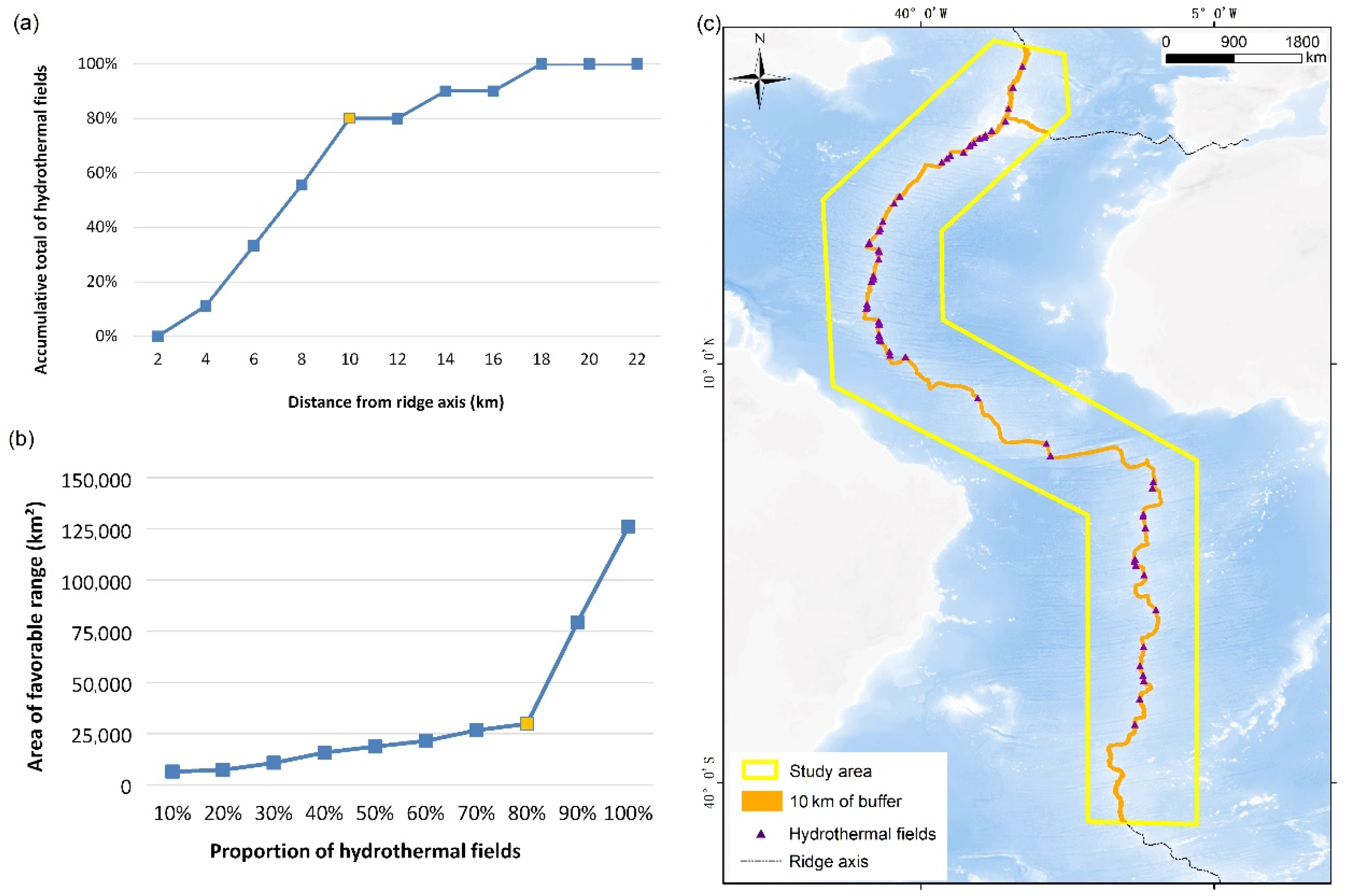
Mid-ocean ridges are places where plates spread and the lithosphere regenerates. Ridge axis data on the Mid-Atlantic Ridge are from the EarthByte Group [28]. According to the distance between the ridge axis and discovered magmatic-related hydrothermal fields in the study area, statistics show that 80% of hydrothermal fields are located within 10 km from the ridge axis, and the number of fields tends to be stable with increasing distances (Figure 6a). The 10 km buffer zone covers 29,842 km² in the study area. When the buffer zone increases, more hydrothermal fields will be covered. However, the area corresponding to this buffer zone will also rise dramatically, which contrasts to the principle that the most training data should locate in the smallest area (Figure 6b). Therefore, a 10 km buffer zone was mapped from the ridge axis (Figure 6c).

Faults

Faults are generally places where stress is concentrated. At the seafloor, some mineral-related substances do not mineralize until they reach a certain distance from the fault, where the stress is low. Therefore, the optimal ore-forming region is the zonal region at a certain distance from a fault, which is called the tectonic buffer zone.

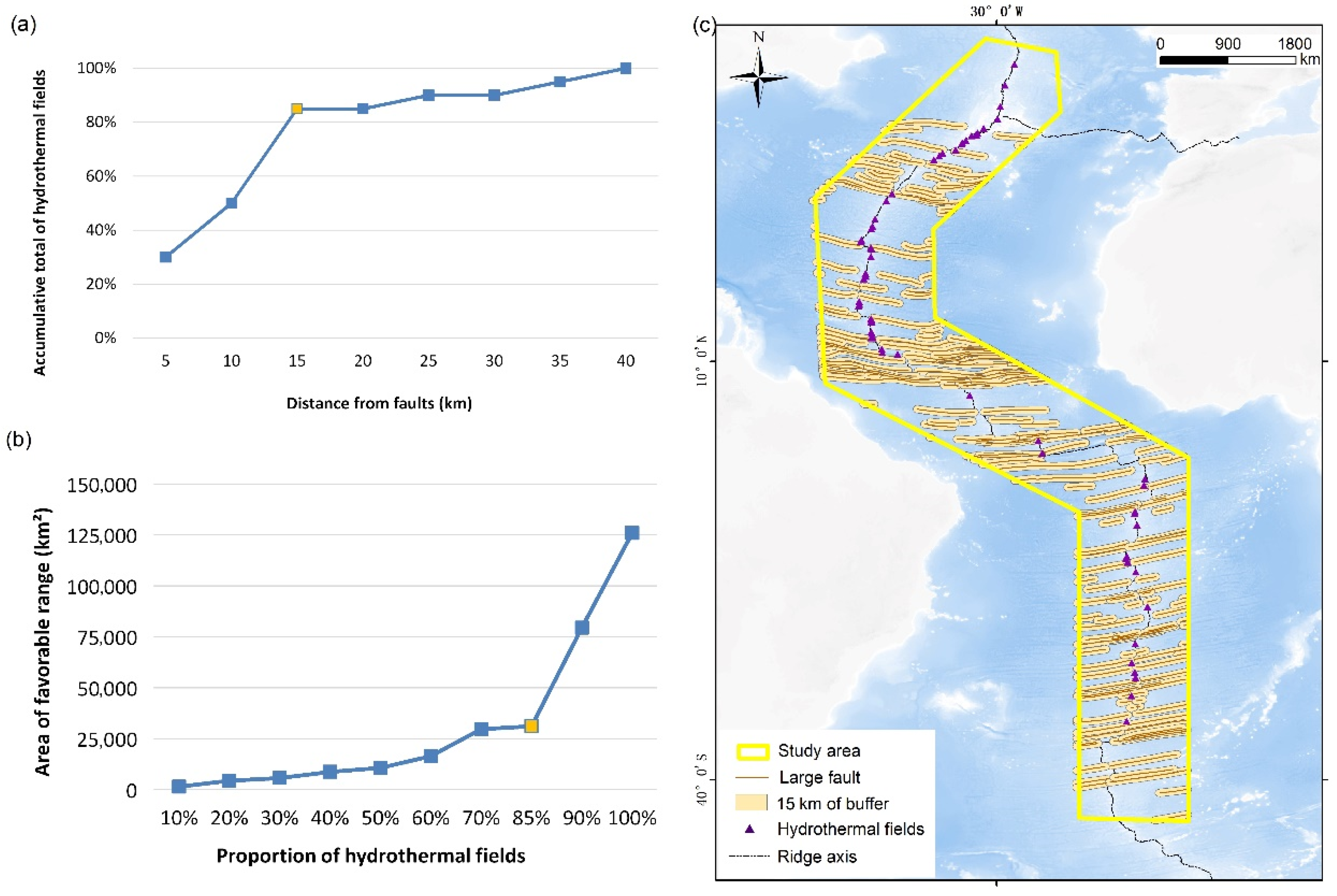
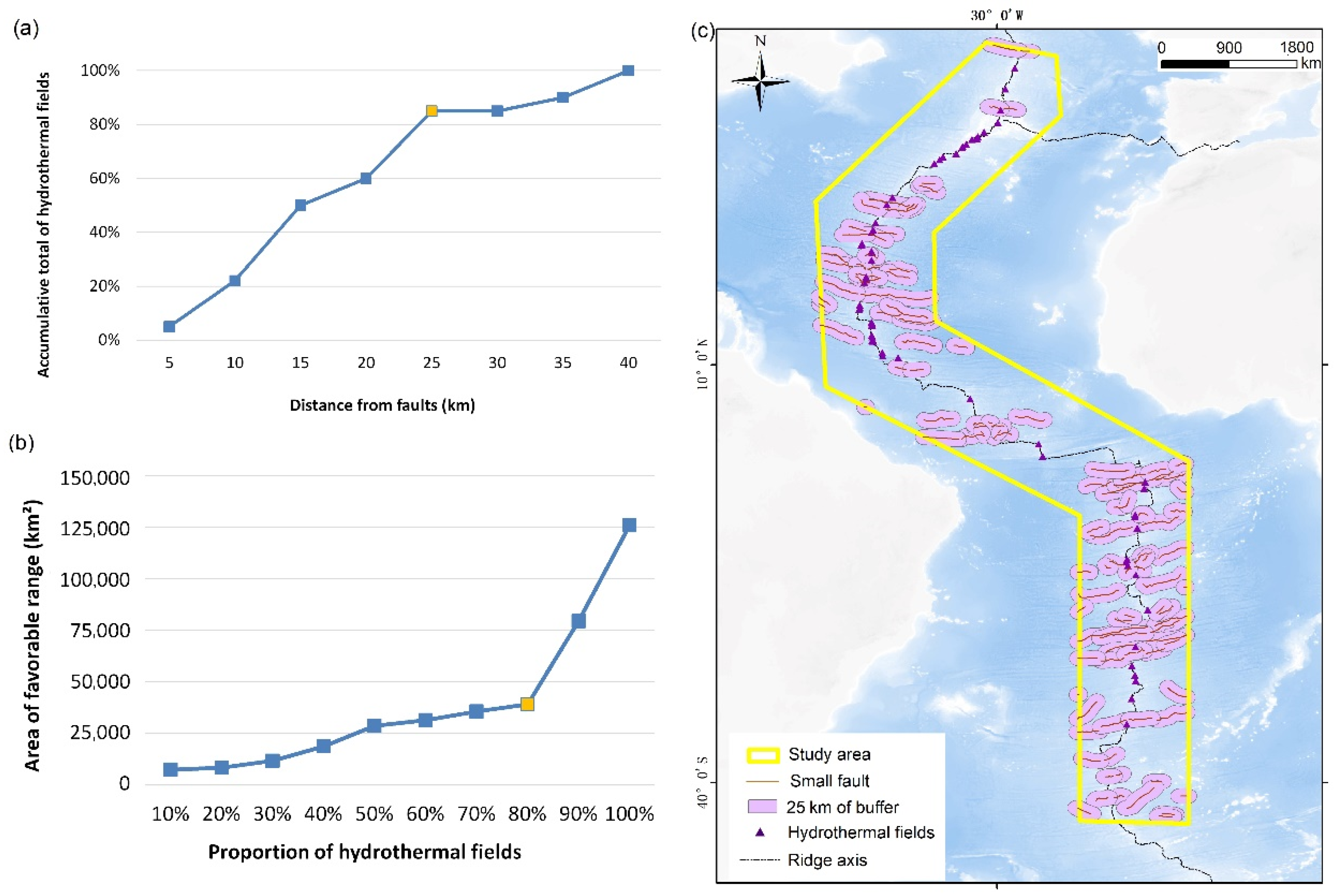
Fault data on the Mid-Atlantic Ridge are from the EarthByte Group [28]. Due to the low spreading rate and low magma supply, the Mid-Atlantic Ridge has a rugged axial terrain and a deep central rift valley [26]. There is frequent tectonic activity, many transform faults, and a large number of normal faults on the ridge. Based on the length of faults with average length of 523 km, fracture zones are classified as large faults with average length of 387 km, and discordant zones are classified as small faults. According to the distance between the large faults and the discovered hydrothermal fields, statistics show that 85% of the hydrothermal fields are located within 15 km of large faults, and the number of fields tends to be stable with increasing distances (Figure 7a). The 15 km buffer zone covers 31,153 km² in the study area. When the buffer zone increases, more hydrothermal fields will be covered. However, the area corresponding to this buffer zone will also rise dramatically, which contrasts to the principle that the most training data should locate in the smallest area (Figure 7b). Therefore, a 15 km buffer zone was mapped from large faults. The method used to determine the buffer zone of small faults was the same (Figure 7c); the buffer for small faults was 25 km (Figure 8).

Bedrock Age

Hydrothermal activities at the seafloor are closely related to the tectonic evolution of oceanic plates. The three oceans began to evolve simultaneously in the Middle Jurassic (171 Ma), and the evolution stages can be divided into four major periods: (1) 171–120 Ma, there is no directional spreading ridge, forming ancient oceanic plates; (2) 120–80 Ma, which belongs to the transitory stage, there is no directional spreading ridge, but volcanism developed widely and formed a large volcanic belt; (3) 80–27 Ma, a linear spreading ridge formed, and young ocean plates began to evolve; and (4) 27–0 Ma, a globally associated spreading ridge was formed. The younger the bedrock of the seafloor, the closer it is to the mid-ocean ridge [29]. This proves that the seafloor is spreading and renewing. The molten magma below the oceanic crust rises along faults and condenses into the new crust. This new crust is being produced constantly and pushes the old crust sideways.

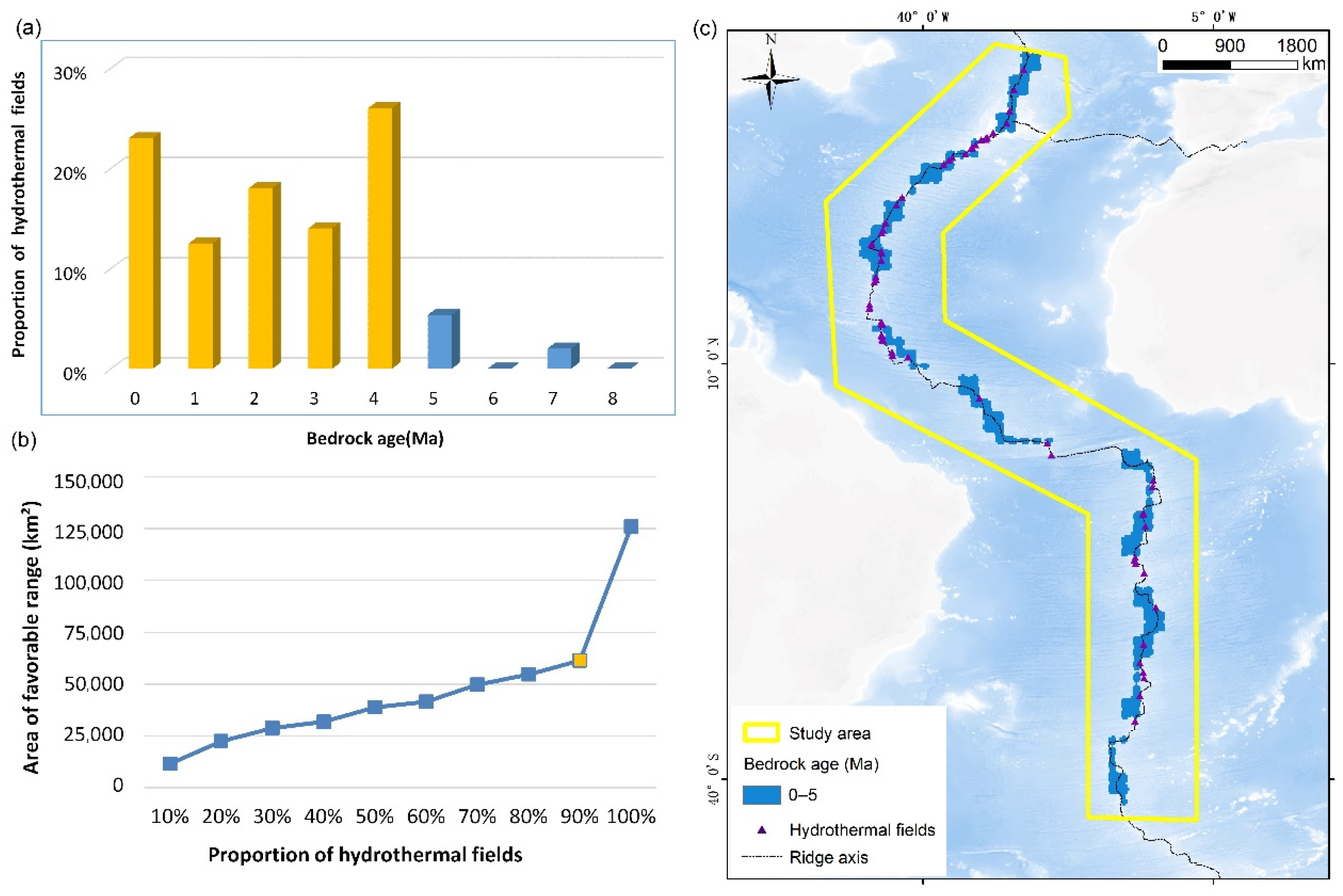
The age of bedrock data is from the NGDC of the NOAA, with a resolution of 2 × 2′ [30]. The hydrothermal activity period of seafloor massive sulfides is generally long, while the mineralization period is relatively short and usually occurs in the late stage of hydrothermal activity. Therefore, the distance between the hydrothermal fields and the ridge can be inferred from the age of the bedrock. On the Mid-Atlantic Ridge, the TAG hydrothermal field is located on the oceanic crust that formed between 100,000 and 200,000 years ago, and its hydrothermal activity is thought to have begun 130,000 years ago [31,32,33]. Statistics of the bedrock age where magmatic-related hydrothermal fields developed in the study area suggest that 93% of magmatic-related hydrothermal fields occurred in areas with bedrock ages ranging from 0 to 5 Ma (Figure 9a). This interval covers 61,348 km² in the study area. When the range increases, more hydrothermal fields will be covered. However, the area corresponding to this range will also rise dramatically, which contrasts the principle that the most training data should locate in the smallest area (Figure 9b). Therefore, the range from 0 to 5 Ma can be used as the favorable interval in the predictive map of bedrock age (Figure 9c).

Spreading Rate

The spreading rate is the dynamic evolution factor controlling the geological process, magma, and tectonics on the mid-ocean ridge. The tectonic environment of mid-oceanic ridges with different spreading rates has different features, including deep magmatic activity, fault structure, and hydrothermal activities. There is a strong linear relationship between the spreading rate and magma supply on the mid-ocean ridge [34]. With the acceleration of the spreading rate, the magma supply increases, and magma activity becomes more frequent [35]; if the spreading rate is relatively low, the magma supply is small and magmatic activities occur less often.

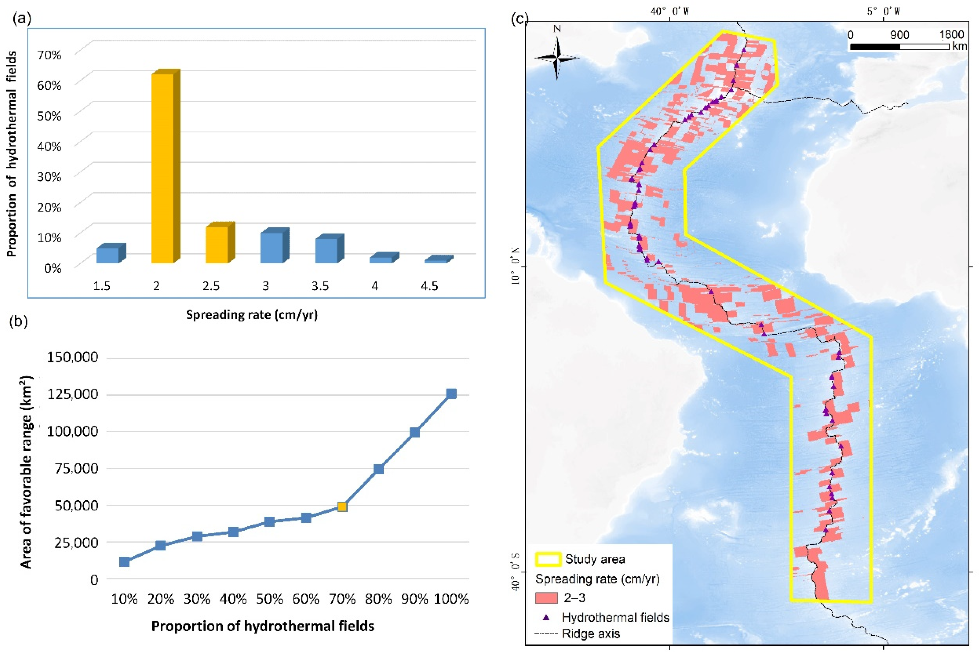
The spreading rate data were obtained from the NOAA NGDC, with a resolution of 2 × 2′. The spreading rate of the Mid-Atlantic Ridge is 2–4 cm/yr, and the spreading rate of the southern Mid-Atlantic Ridge is faster than that of the northern Mid-Atlantic Ridge. However, the spreading rate of the southern Mid-Atlantic Ridge is decreasing while that of the northern Mid-Atlantic Ridge is increasing. Generally speaking, the Mid-Atlantic Ridge is a typical symmetric spreading ridge. Statistics of the spreading rate where magmatic-related hydrothermal fields developed in the study area suggest that 74% of hydrothermal fields occurred in areas with spreading rates ranging from 2 to 3 cm/yr (Figure 10a). This interval covers 48,941 km² in the study area. When the range increases, more hydrothermal fields will be covered. However, the area corresponding to this range will also rise dramatically, which contrasts the principle that the most training data should locate in the smallest area (Figure 10b). Therefore, 2 to 3 cm/yr can be used as the favorable interval in the predictive map of the spreading rate (Figure 10c).

4.1.4. Geophysical Information

Bouguer Gravity

Bouguer gravity can be used to explore seafloor massive sulfide deposits through the density difference between the target orebody and the wall rock. The seafloor massive sulfides mainly contain sphalerite, pyrite, chalcopyrite, and pyrrhotite [36,37]. The wall rock is generally mid-ocean ridge basalt, and some areas are covered by sediments [37]. The mineral density of seafloor massive sulfides is clearly higher than that of basalt. Therefore, the Bouguer gravity anomaly in the seafloor massive sulfide enrichment area shows a local abnormally high value region, which is the direct manifestation of a seafloor massive sulfide deposit in the Bouguer gravity anomaly.

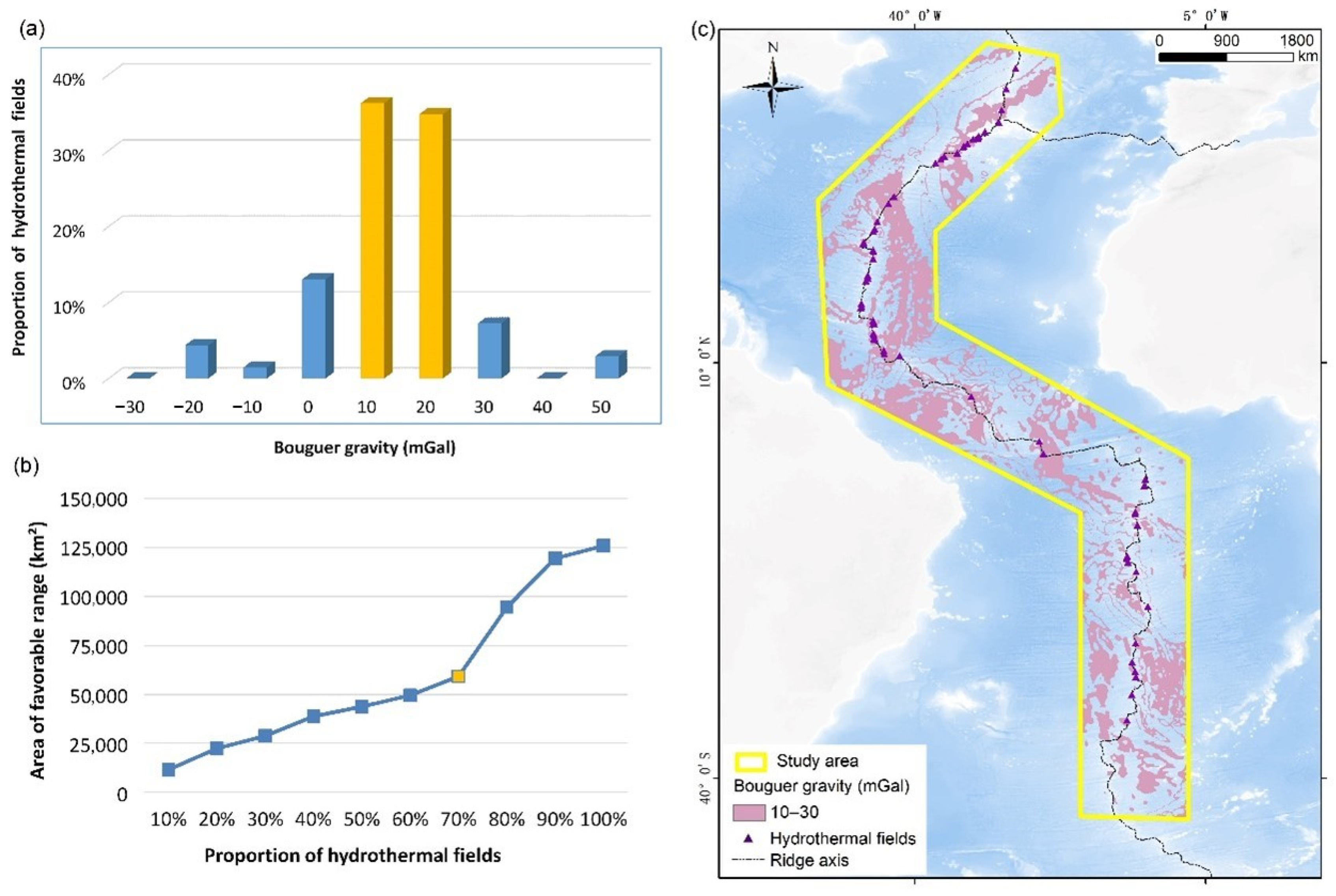
The Bouguer gravity data are from the WGM2012 Global Gravity Anomaly Data Model established by the International Geomagnetic Agency (BGI) [38], with a resolution of 2 × 2′. The variation trend of Bouguer gravity in the study area is consistent with the water depth. The Bouguer gravity value is higher near the mid-ocean ridge, up to 30 mGal, and decreases gradually away from it [39]. Statistics of the Bouguer gravity where magmatic-related hydrothermal fields developed in the study area suggest that 71% of these fields occurred in areas with Bouguer gravity ranging from 10 to 30 mGal (Figure 11a). This interval covers 59,141 km² in the study area. When the range increases, more hydrothermal fields will be covered. However, the area corresponding to this range will also rise dramatically, which contrasts the principle that the most training data should locate in the smallest area (Figure 11b). Therefore, 10 to 30 mGal can be used as the favorable interval in the predictive map of Bouguer gravity (Figure 11c).

Magnetism

The titanomagnetite in volcanic lava erupting from the rift valley is the main reason for the residual magnetization near the mid-ocean ridge. However, titanomagnetite can be easily altered owing to the acidic hydrothermal fluid, and the abundance of magnetite in the rocks of the oceanic crust decreases. Therefore, when a hydrothermal system is under altered crust, the magnetic intensity of the altered crust is lower than that of the original state. Low magnetic intensity is an important prospecting indicator in the exploration of seafloor massive sulfides [19].

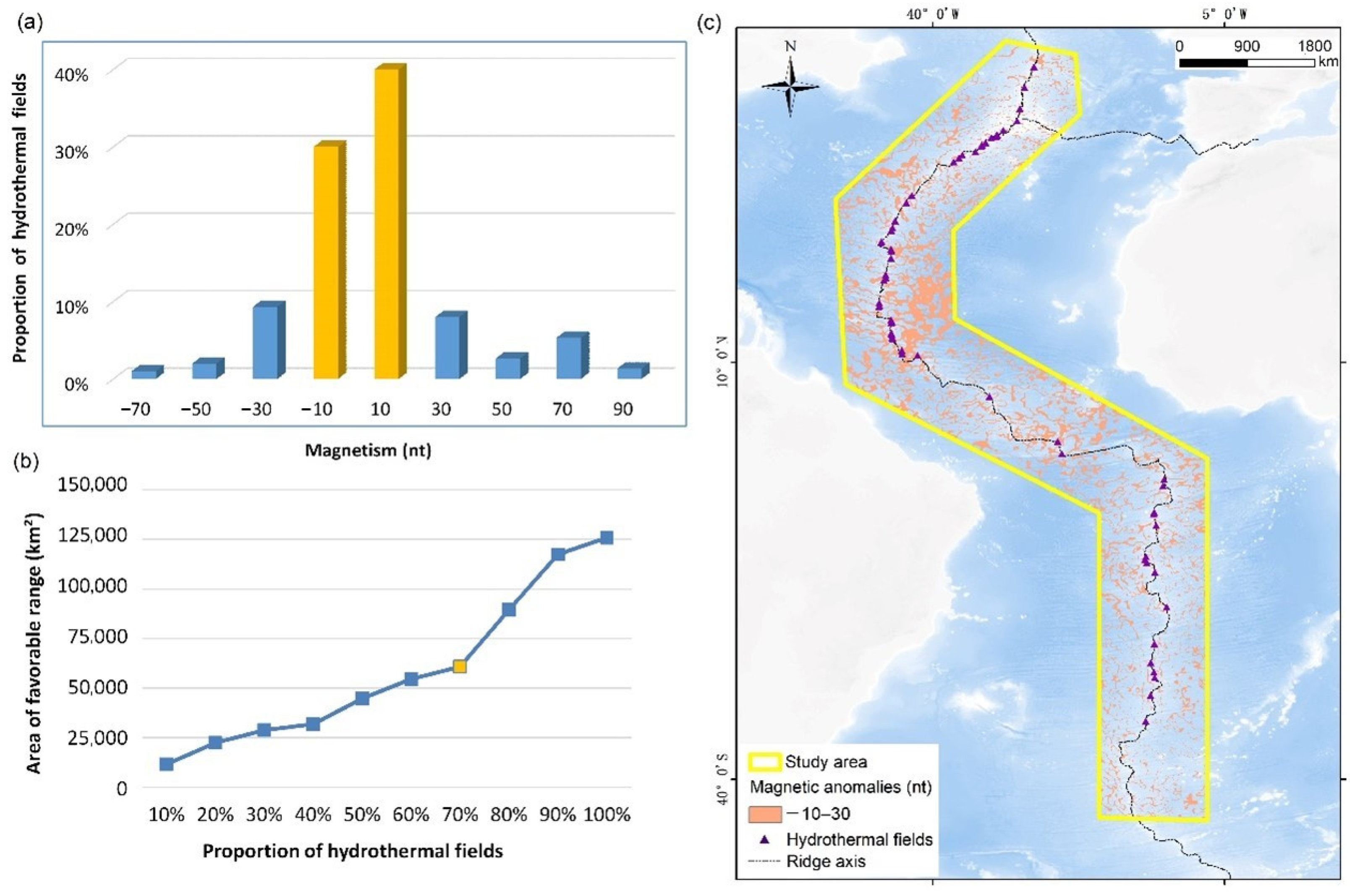
The magnetic data were obtained from the Global Magnetic Anomaly Grid Model (EMAG2), published by the Cooperative Institute for Environmental Sciences at the University of Colorado (CIRES), with a resolution of 2 × 2′ [40]. The magnetic anomalies of the Atlantic are distributed along the mid-ocean ridge, primarily in the north and west directions, with alternating positive and negative anomalies. Statistics of the magnetic data where magmatic-related hydrothermal fields developed in the study area suggest that 70% of magmatic-related hydrothermal fields occurred in areas with magnetism ranging from −10 to 30 nt (Figure 12a). This interval covers 60,802 km² in the study area. When the range increases, more hydrothermal fields will be covered. However, the area corresponding to this range will also rise dramatically, which contrasts the principle that the most training data should locate in the smallest area (Figure 12b). Therefore, this range can be used as the favorable interval in the predictive map of magnetism (Figure 12c).

Seismic Point Density

Seismic and volcanic events on the seafloor indicate that the regional crustal is active due to magma and faults in the area [41]. Magma supply is the most important heat source for hydrothermal activities, and faults provide channels for hydrothermal circulation. The existence of heat sources and hydrothermal circulation channels are two basic conditions for the generation of seafloor massive sulfides; therefore, seismic activities indirectly indicate the existence of these deposits. Every earthquake is accompanied by the collapse of an old chimney and the formation of a new chimney, and many seafloor hydrothermal systems are located on volcanoes [42].

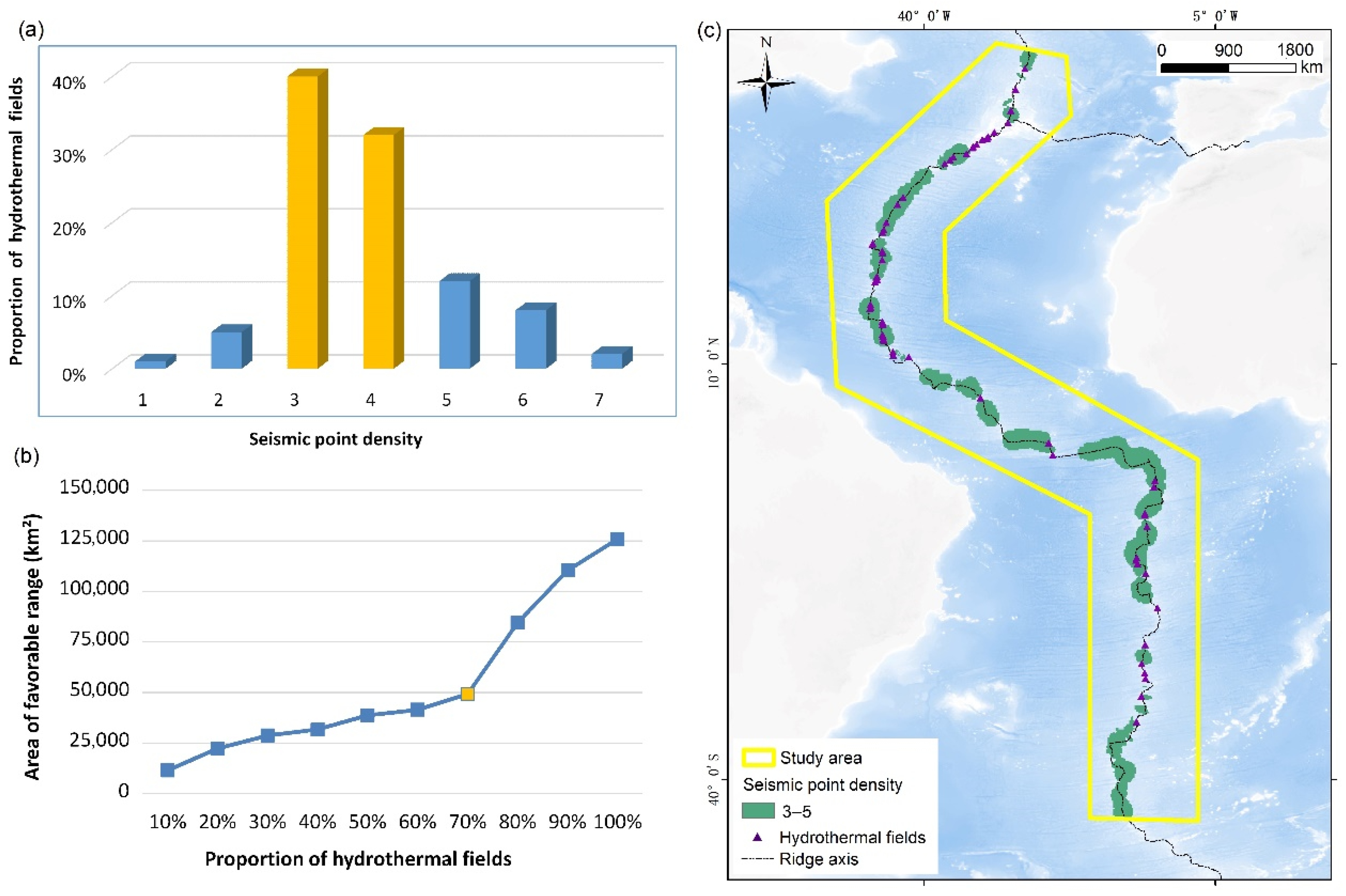
The seismic data are from the United States Geological Survey (USGS) and include earthquake events with magnitudes greater than five from 1950 to 2013. First, the point density of the seismic data was calculated. Since a magnitude 6 earthquake is five times as strong as a magnitude 5 earthquake, and so on, the magnitude of the earthquake was taken into account when calculating the density of seismic points. Statistics of the seismic point density where magmatic-related hydrothermal fields developed in the study area suggest that 72% of magmatic-related hydrothermal fields occurred in areas with seismic point densities ranging from 3 to 5 (Figure 13a). This interval covers 49,271 km² in the study area. When the range increases, more hydrothermal fields will be covered. However, the area corresponding to this range will also rise dramatically, which contrasts the principle that the most training data should locate in the smallest area (Figure 13b). Therefore, the range from 3 to 5 can be used as the favorable interval in the predictive map of seismic point density (Figure 13c).

4.2. Mineral Potential Model of Seafloor Massive Sulfide Deposits

Based on the extraction of favorable intervals for the mineralization of magmatic-related seafloor massive sulfides on the Mid-Atlantic Ridge, 3 types of predictive maps with a total of 11 factors were obtained. By combining these predictive maps, a quantitative mineral potential model was established (

Table 2. Mineral potential model of seafloor massive sulfide.

Ore-Controlling Factors	Characteristic Variables	Favorable Range
Terrain Information	Water depth	[−3000, −2500] m
	Slope gradient	[5, 25]°
Geology Information	Oceanic crust thickness	[7600–8500] m
	Large faults	15 km buffer
	Small faults	25 km buffer
	Ridge axis	10 km buffer
	Bedrock age	[0, 5] Ma
	Spreading rate	[2, 2.5] cm/yr
Geophysical Information	Bouguer gravity	[10, 30] mGal
	Magnetism	[−10, 30] nt
	Seismic point density	[3, 5]

).

5. Mineral Prospectivity Mapping

The weights-of-evidence method was adopted for the mineral prospectivity mapping of magmatic-related seafloor massive sulfides on the Mid-Atlantic Ridge. Proposed by the Canadian geologist Agterberg, weights-of-evidence is a linear model based on the Bayes theorem. It can calculate the relative importance of predictive maps using a statistical geologic method and estimate the location of potential deposits. The main formula and process of weights-of-evidence method are as follows [18].

First, the study area is divided into T small unit cells, whose size is sufficiently small so that one unit cell usually contains only one deposit [43]. If there are D known deposits, there are D unit cells that contain one deposit. Then, the prior probability that a unit cell chosen at random is P(D) = D/T, expressed as a priori odds by:

$$O\left(D\right)=\frac{P\left(D\right)}{1-P\left(D\right)}=\frac{D}{T-D}$$

(1)

If there are n predictive maps, for the jth binary predictive map, j = 1,2 n, the number of unit cells where the predictive map is present is B_j. The weight for the jth predictive map can be defined as:

$$W_j^{+}=\ln \frac{P\left(B_j\mid D\right)}{P\left(B_j\mid \overline{D}\right)}$$

(2)

$$W_j^{-}=\ln \frac{P\left({\overline{B}}_j\mid D\right)}{P\left({\overline{B}}_j\mid \overline{D}\right)}$$

(3)

where W+ is a positive weight indicating the predictive map is present, while W− is a negative weight indicating the predictive map is absent in the unit cell. W values:

$$W_j=W_j^{+}-W_j^{-}$$

(4)

can be used to define the strength of the association between deposits and predictive maps.

Assuming predictive maps are conditionally independent, all weights can be summed up to find the natural logarithm of posterior odds of potential deposits as given by:

$$\ln \left\{O_{\mathrm{Posterior}}\left(\mathrm{D}\mid {\mathrm{B}}_1^{\mathrm{k}}\cap {\mathrm{B}}_2^{\mathrm{k}}\cap {\mathrm{B}}_3^{\mathrm{k}}\dots {\mathrm{B}}_{\mathrm{n}}^{\mathrm{k}}\right)\right\}={\displaystyle \sum }_{j=1}^{\mathrm{n}}{W}_j^k+\ln O_{\mathrm{Pr}\mathrm{ior}}\left(D\right)\left(j=1,2,3,\dots ,n\right)$$

(5)

where $W_j^k$ is the weight of the jth predictive map, and k is either a positive or negative weighting depending on whether or not the jth predictive map is present. Given this, posterior probability values can be calculated using:

$$P_{\mathrm{Posterior}}=O_{\mathrm{Posterior}}/\left(1+O_{\mathrm{Posterior}}\right)$$

(6)

In this study, we divided the study area into unit cells with a side of 50 km. Then, the weight of each predictive map was estimated by Equations (2)–(4). According to the weight values in

Table 3. Table of predictors’ weight.

Ore-Controlling Factors	Evidence Factors	W+	W−	W
Terrain Information	Water depth	0.66	−1.05	1.72
	Slope gradient	1.43	−0.44	1.87
Geology Information	Oceanic crust thickness	2.12	−1.50	3.62
	Large faults	1.99	−1.45	3.44
	Small faults	1.71	−0.55	2.26
	Ridge axis	1.43	−0.44	1.87
	Bedrock age	1.59	0.00	1.59
	Spreading rate	0.79	−2.60	3.39
Geophysical Information	Bouguer gravity	0.16	−0.26	0.43
	Magnetism	0.04	−0.22	0.26
	Seismic point density	0.72	−0.55	1.28

, the oceanic crust thickness has the highest weight value (3.62), and the predictive map with the next highest weight value is the buffer zone of large faults with a weight value of 3.44, followed by the spreading rate (3.39). This result suggests that these three predictive maps have a close relationship with the formation of seafloor massive sulfide deposits. Therefore, they are important prospecting criteria for magmatic-related seafloor massive sulfides on the Mid-Atlantic Ridge.

In order to apply the weights-of-evidence method successfully, predictive maps must be conditionally independent, and the data population of each predictive map should have a normal distribution. In this study, the chi-squared statistic (χ2) was used to ensure independency, with a theoretical value of 3.84 with 1 degree of freedom at a level α = 0.05.

Table 4. Pairwise χ2 tests for conditional independence of 11 predictor.

	Water Depth	Slope Gradient	Oceanic Crust Thickness	Large Faults	Small Faults	Ridge Axis	Bedrock Age	Spreading Rate	Bouguer Gravity	Magnetism	Seismic Point Density
Water Depth
Slope Gradient	0.79
Oceanic Crust Thickness	2.65	1.89
Large Faults	2.11	0.76	2.56
Small Faults	0.69	0.62	2.13	0.73
Ridge Axis	3.44	1.58	3.12	2.04	1.23
Bedrock Age	2.91	2.19	1.84	3.45	2.7	0.93
Spreading Rate	1.78	2.39	3.69	2.65	1.86	0.81	1.12
Bouguer Gravity	1.67	3.81	1.04	2.78	0.94	0.78	2.15	1.16
Magnetism	2.94	1.15	2.3	1.67	1.91	1.81	2.04	0.81	0.89
Seismic Point Density	2.25	1.27	1.84	1.38	2.26	0.93	0.14	1.62	1.19	1.31

shows that all estimated χ2 values of the 11 predictive maps are below theoretical values, indicating that the predictive maps satisfy conditional independency.

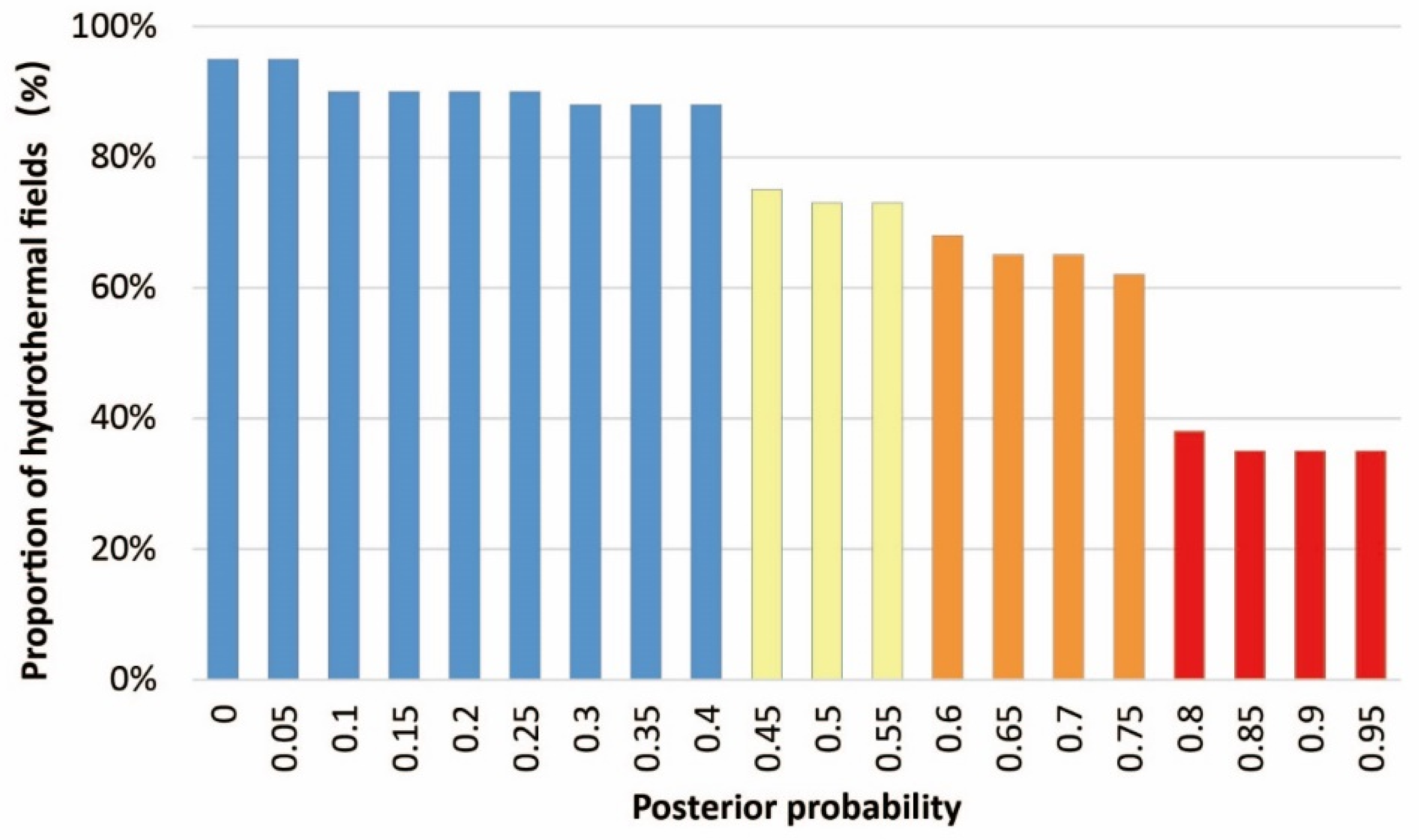
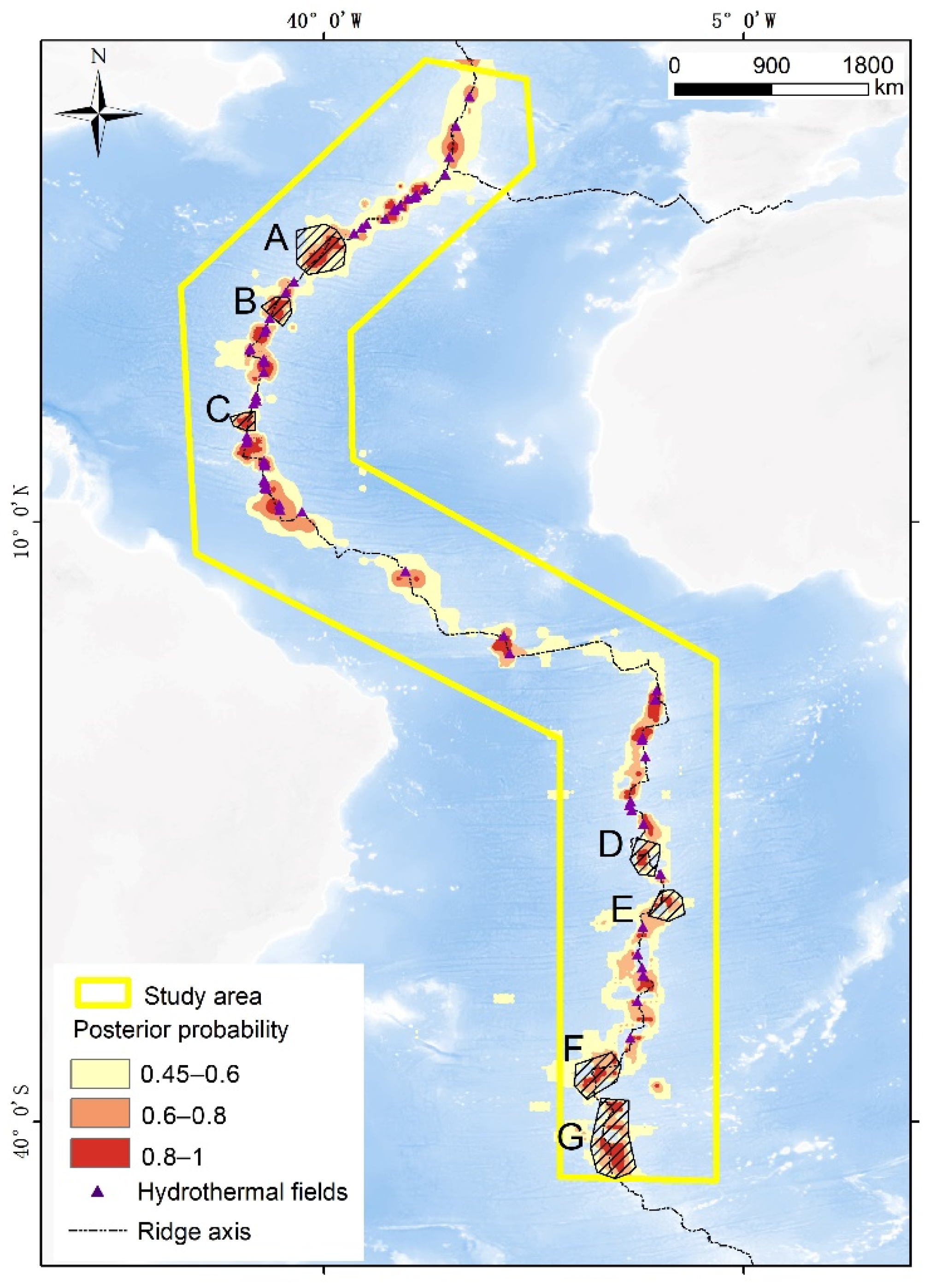
The posterior probability of each grid was calculated according to Equation (5), in which higher values of posterior probability represent a greater probability for finding seafloor massive sulfides. The relationship between the value of posterior probability and the percentage of contained hydrothermal fields is shown in Figure 14. When the value of posterior probability is 0.8, the proportion of known hydrothermal fields contained in the area of posterior probability below 0.8 changes abruptly, and when the posterior probability is above 0.8, the proportion of known hydrothermal fields covered becomes relatively stable. Thus, 0.8 can serve as a predictive threshold. We delineated 7 prospecting targets with values of posterior probability over 0.8 outside the regions of known hydrothermal fields (Figure 15).

6. Discussion

6.1. Important Prospecting Criteria

According to the weight values in Table 3, oceanic crust thickness, large faults, and spreading rate are the three most important prospecting criteria for magmatic-related seafloor massive sulfides on the Mid-Atlantic Ridge, among which large faults are the reflection of tectonic activities, while the oceanic crust thickness and spreading rate reflect the magmatic activities.

On slow-spreading ridges, large faults, oceanic crust thickness, and spreading rate are also important prospecting criteria for magmatic-related seafloor massive sulfides. Compared to fast and intermediate-spreading ridges, slow-spreading ridges differ in fault characteristics [44]. On fast-spreading ridges, abundant magmatic activities result in uplift at the top of the ridge, and because of the extrusion on both ridge flanks, there are fewer normal faults with inward dipping. The shallow depth of faulting and restricted hydrothermal circulation channels lead to fewer faults favoring ore formation [45]. In contrast, slow-spreading ridges are characterized by large scale and deep dipping faults, allowing hydrothermal fluids to deeply circulate and interact with wall rocks. In addition, magmatic activities are another important prospecting criterion for massive magmatic-related seafloor sulfides on slow-spreading ridges. Magma is the heat source for hydrothermal circulation [46]. On fast-spreading and intermediate-spreading ridges, the magma supply is strong [47,48], while with slow-spreading ridges, magma is enriched under neo-volcanic ridges [49].

In conclusion, important prospecting criteria for magmatic-related seafloor massive sulfide deposits on the Mid-Atlantic Ridge found in this paper are similar to those for other slow-spreading ridges. Therefore, the Mid-Atlantic Ridge is considered a typical slow-spreading ridge.

6.2. Prospecting Targets

The mineral prospecting mapping combined three types of data with the location of known magmatic-related hydrothermal fields to identify areas with a high potential for future mineral exploration on the Mid-Atlantic Ridge. In regions outside known hydrothermal fields, we delineated seven targets, among which targets A, B, and C are on the northern Mid-Atlantic Ridge, and D, E, F, and G are on the southern Mid-Atlantic Ridge. These prospecting targets can be considered priority exploration areas for seafloor massive sulfides.

On the northern Mid-Atlantic Ridge, prospecting target A is located near 32.5° N, which is in the south of the seafloor plateau formed by the Azores hot spot. Due to the interaction between ridges and hot spots, the ridge segment of prospecting target A has stronger magmatic activities and thicker oceanic crust than its southern ridge segments. There are 4 known hydrothermal fields around prospecting target A. Prospective target B is near 27.7° N and located in the shallowest second-order ridge segment between the Atlantis and Kane transform faults [50]. Its topography is similar to a ‘bathtub’. Fresh vitreous pillow basalt is distributed along the ridge and is covered with thin deep-sea sediment. Famous hydrothermal fields such as Broken Spur and TAG are around prospective target B [51,52]. Target C is in the middle of the northern Mid-Atlantic Ridge. There are many irregular faults along the ridge, and the depth of the terrain deepens from 3600 to 4300 m from ridge to flanks. Target C belongs to an active seismic zone. There are four famous hydrothermal fields: 24°30′ N, Snake Pit, Tamar, and Zenith Victory, from north to south, around prospecting target C, among which the first two hydrothermal fields are active, and activity in the last two has ceased [53,54].

On the southern Mid-Atlantic Ridge, prospecting target D is near 13.5° S and near new volcanoes. Its water depth ranges from 2000 to 3000 m, and the terrain fluctuates greatly. SMAR 14° S and 15° S hydrothermal fields are in the north of prospecting target D, and the SMAR 19° S hydrothermal field is in the south [55]. Prospecting target E lies between the Martin Bac and SMAR 22° S transform fault. North-south strike faults develop at prospecting target E, which is also near Saint Helena volcanic islands. Therefore, prospecting target E has frequent tectonic and magmatic activities, which are favorable for seafloor massive sulfide mineralization. Prospecting target F and G are near 35.5° S and 40.5° S, which are at the southern end of the study area. MAR 33° S is to the north of prospecting target F. The water depth of prospecting F and G are shallow and there is neovolcanic zone on their shallowest portion of the ridge cross section. On such broad and shallow regions, it is likely that hydrothermal fields occur as low-temperature, diffuse flow [9].

7. Conclusions

This study established a quantitative mineral potential model of magmatic-related seafloor massive sulfides on the Mid-Atlantic Ridge for the first time. This model contains 11 predictive maps, including water depth, slope, oceanic crust thickness, large faults, small faults, ridge, bedrock age, spreading rate, Bouguer gravity, and magnetic and seismic point density. The weight values of predictive maps show that the thickness of the oceanic crust, large faults, and spreading rate are the most important prospecting criteria, followed by small faults, ridge, and slope gradient, which are the same on other typical slow-spreading ridges. Therefore, the quantitative mineral potential model in this study is also appropriate for other typical slow-spreading ridges. In addition, seven prospecting targets with high posterior probabilities were delineated, which provides a basis for the position of magmatic-related seafloor massive sulfides on the Mid-Atlantic Ridge.

References

- Tao, C.; Li, H.; Jin, X.; Zhou, J.; Wu, T.; He, Y.; Deng, X.; Gu, C.; Zhang, G.; Liu, W. Seafloor hydrothermal activity and polymetallic sulfide exploration on the southwest Indian ridge. Chin. Sci. Bull. 2014, 59, 2266–2276. [Google Scholar] [CrossRef]
- Hannington, M.; Jamieson, J.; Monecke, T.; Petersen, S. Estimating the Metal Content of SMS Deposits 2011; IEEE: Piscataway, NJ, USA, 2011; pp. 1–4. [Google Scholar]
- Corliss, J.B.; Dymond, J.; Gordon, L.I.; Edmond, J.M.; von Herzen, R.P.; Ballard, R.D.; Green, K.; Williams, D.; Bainbridge, A.; Crane, K. Submarine thermal springs on the Galapagos Rift. Science 1979, 203, 1073–1083. [Google Scholar] [CrossRef] [PubMed]
- Beaulieu, S.E.; Baker, E.T.; German, C.R. Where are the undiscovered hydrothermal vents on oceanic spreading ridges? Deep Sea Res. Part II Top. Stud. Oceanogr. 2015, 121, 202–212. [Google Scholar] [CrossRef] [Green Version]
- Dai, Y.; Liu, S.J.; Liu-Jun, L.I.; Xiao-Zhou, H.U. Sampling techniques and equipments for sms exploration by nautilus minerals inc. Mar. Geol. Quat. Geol. 2008, 29, 863–870. [Google Scholar]
- Jie, F.; Jingwen, S.; Hongqing, X.; Jinhua, Y.; Jianping, C.; Mengyi, R.; Chao, T. Mineral prospectivity mapping of seafloor massive sulfide on the Northern Mid-Atlantic Ridge. Adv. Earth Sci. 2015, 30, 60–68. (In Chinese) [Google Scholar]
- Ke, S. Quantitative Prediction and Evaluation of Seafloor Massive Sulfide in the North Atlantic Ocean; China University of Geosciences: Beijing, China, 2016. (In Chinese) [Google Scholar]
- Kleinrock, M.C.; Humphris, S.E. Structural asymmetry of the TAG Rift Valley: Evidence from a near-bottom survey for episodic spreading. Geophys. Res. Lett. 2013, 23, 3439–3442. [Google Scholar] [CrossRef]
- Devey, C.W.; German, C.R.; Haase, K.M.; Lackschewitz, K.S.; Melchert, B.; Connelly, D.P. The Relationships between Volcanism, Tectonism, and Hydrothermal Activity on the Southern Equatorial Mid-Atlantic Ridge. In Diversity of Hydrothermal Systems on Slow Spreading Ocean Ridge; American Geophysical Union: Washington, DC, USA, 2013. [Google Scholar]
- Fouquet, Y. Where are the large hydrothermal sulphide deposits in the oceans? Philos. Trans. R. Soc. Lond. Ser. A 1997, 355, 427–441. [Google Scholar] [CrossRef]
- Humphris, S.E.; Kleinrock, M.C. Detailed morphology of the TAG Active Hydrothermal Mound: Insights into its formation and growth. Geophys. Res. Lett. 2013, 23, 3443–3446. [Google Scholar] [CrossRef]
- Demartin, B.J.; Sohn, R.A.; Canales, J.P.; Humphris, S.E. Kinematics and geometry of active detachment faulting beneath the Trans-Atlantic Geotraverse (TAG) hydrothermal field on the Mid-Atlantic Ridge. Geology 2007, 35, 711–714. [Google Scholar] [CrossRef] [Green Version]
- Fouquet, Y.; Cambon, P.; Etoubleau, J.; Charlou, J.L.; OndréAs, H.; Barriga, F.J.; Cherkashov, G.; Semkova, T.; Poroshina, I.; Bohn, M. Geodiversity of Hydrothermal Processes along the Mid-Atlantic Ridge and Ultramafic-Hosted Mineralization: A New Type of Oceanic Cu-Zn-Co-Au Volcanogenic Massive Sulfide Deposit; Wiley-Blackwell: Hoboken, NJ, USA, 2013; pp. 321–367. [Google Scholar]
- Canales, J.P.; Sohn, R.A.; Demartin, B.J. Crustal structure of the Trans-Atlantic Geotraverse (TAG) segment (Mid-Atlantic Ridge, 26°10′ N): Implications for the nature of hydrothermal circulation and detachment faulting at slow spreading ridges. Geochem. Geophys. Geosyst. 2007, 8. [Google Scholar] [CrossRef]
- Garcés, M.; Gee, J.S. Paleomagnetic evidence of large footwall rotations associated with low-angle faults at the Mid-Atlantic Ridge. Geology 2007, 35, 279–282. [Google Scholar] [CrossRef]
- Lowell, R.P.; Rona, P.A. Seafloor hydrothermal systems driven by the serpentinization of peridotite. Geophys. Res. Lett. 2002, 29, 21–26. [Google Scholar] [CrossRef] [Green Version]
- McCaig, A.M.; Delacour, A.; Fallick, A.E.; Castelain, T.; Früh-Green, G.L. Detachment fault control on hydrothermal circulation systems: Interpreting the subsurface beneath the TAG hydrothermal field using the isotopic and geological evolution of oceanic core complexes in the Atlantic. Divers. Hydrothermal. Syst. Slow Spreading Ocean. Ridges Geophys. Monogr. Ser. 2010, 188, 207–240. [Google Scholar]
- Bonham-Carter, G.F. Geographic Information Systems for Geoscientists: Modelling with GIS; Elsevier: Amsterdam, The Netherlands, 1994. [Google Scholar]
- Tivey, M.A.; Dyment, J. The magnetic signature of hydrothermal systems in slow spreading environments. Divers. Hydrothermal. Syst. Slow Spreading Ocean. Ridges Geophys. Monogr. Ser. 2010, 188, 43–65. [Google Scholar]
- Cann, J.R.; Strens, M.R. Modeling periodic megaplume emission by black smoker systems. J. Geophys. Res. Solid Earth 1989, 94, 12227–12237. [Google Scholar] [CrossRef]
- Lim, E.; Eakins, B.; Taylor, L.A. Challenges Integrating Bathymetric and Topographic Datasets of American Samoa. AGUFM 2009, 2009, U21E-2188. [Google Scholar]
- Bougault, H.; Charlou, J.L.; Fouquet, Y.; Needham, H.D.; Vaslet, N.; Appriou, P.; Baptiste, P.J.; Rona, P.A.; Dmitriev, L.; Silantiev, S. Fast and slow spreading ridges—Structure and hydrothermal activity, ultramafic topographic highs, and CH4 output. J. Geophys. Res. Solid Earth 1993, 98, 9643. [Google Scholar] [CrossRef]
- Gràcia, E.; Escartín, J. Crustal accretion at mid-ocean ridges and backarc spreading centers: Insights from the Mid-Atlantic Ridge, the Bransfield Basin and the North Fiji Basin. Contrib. Sci. 2000, 1, 175–192. [Google Scholar]
- Liu, L.; Lowell, R.P. Models of hydrothermal heat output from a convecting, crystallizing, replenished magma chamber beneath an oceanic spreading center. J. Geophys. Res. Solid Earth 2009, 114, B02102. [Google Scholar] [CrossRef] [Green Version]
- Baker, E.T.; Chen, Y.J.; Morgan, J.P. The relationship between near-axis hydrothermal cooling and the spreading rate of mid-ocean ridges. Earth Planet. Sci. Lett. 1996, 142, 137–145. [Google Scholar] [CrossRef]
- Cannat, M.; Briais, A.; Deplus, C.; Escart, N.J.; Georgen, J.; Lin, J.; Mercouriev, S.; Meyzen, C.; Muller, M.; Pouliquen, G. Mid-Atlantic Ridge–Azores hotspot interactions: Along-axis migration of a hotspot-derived event of enhanced magmatism 10 to 4 Ma ago. Earth Planet. Sci. Lett. 1999, 173, 257–269. [Google Scholar] [CrossRef]
- White, R.S.; Minshull, T.A.; Bickle, M.J.; Robinson, C.J. Melt generation at very slow-spreading oceanic ridges: Constraints from geochemical and geophysical data. J. Pet. 2001, 42, 1171–1196. [Google Scholar] [CrossRef] [Green Version]
- Matthews, K.J.; Müller, R.D.; Wessel, P.; Whittaker, J.M. The tectonic fabric of the ocean basins. J. Geophys. Res. Atmos. 2011, 116, B12109. [Google Scholar] [CrossRef] [Green Version]
- Peucker Ehrenbrink, B.; Miller, M.W. Quantitative bedrock geology of east and Southeast Asia (Brunei, Cambodia, eastern and southeastern China, East Timor, Indonesia, Japan, Laos, Malaysia, Myanmar, North Korea, Papua New Guinea, Philippines, far-eastern Russia, Singapore, Korea, Taiwan, Thailand, Vietnam). Geochem. Geophys. Geosyst. 2004, 5, Q01B06. [Google Scholar]
- Müller, R.D.; Sdrolias, M.; Gaina, C.; Roest, W.R. Age, spreading rates, and spreading asymmetry of the world’s ocean crust. Geochem. Geophys. Geosyst. 2008, 9, Q04006. [Google Scholar] [CrossRef]
- Rona, P.A.; Scott, S.D. A special issue on sea-floor hydrothermal mineralization; new perspectives; preface. Econ. Geol. 1993, 88, 1935–1976. [Google Scholar] [CrossRef]
- Humphris, S.E.; Tivey, M.K. A synthesis of geological and geochemical investigations of the TAG hydrothermal field: Insights into fluid-flow and mixing processes in a hydrothermal system. Spec. Pap. Geol. Soc. Am. 2000, 349, 213–235. [Google Scholar]
- Hannington, M.D.; Jamieson, J.; Monecke, T.; Petersen, S. Modern Sea-Floor Massive Sulfides and Base Metal Resources: Toward an Estimate of Global Sea-Floor Massive Sulfide Potential; Society of Economic Geologists: Littleton, CO, USA, 2010. [Google Scholar]
- Reid, I.D.; Jackson, H.R. Oceanic spreading rate and crustal thickness. Mar. Geophys. Res. 1981, 5, 165–172. [Google Scholar]
- Chen, Y.J. Oceanic crustal thickness versus spreading rate. Geophys. Res. Lett. 2013, 19, 753–756. [Google Scholar] [CrossRef]
- Tucholke, B.E.; Lin, J.; Kleinrock, M.C.; Tivey, M.A.; Reed, T.B.; Goff, J.; Jaroslow, G.E. Segmentation and crustal structure of the western Mid-Atlantic Ridge flank, 25°25′–27°10′ N and 0–29 m.y. J. Geophys. Res. Solid Earth 1997, 102, 10203–10223. [Google Scholar] [CrossRef] [Green Version]
- Sauter, D.; Sloan, H.; Cannat, M.; Goff, J.; Patriat, P.; Schaming, M.; Roest, W.R. From slow to ultra-slow: How does spreading rate affect seafloor roughness and crustal thickness? Geology 2011, 39, 911–914. [Google Scholar] [CrossRef]
- Bonvalot, S.; Balmino, G.; Briais, A.; Kuhn, M.; Peyrefitte, A.; Vales, N.; Biancale, R.; Gabalda, G.; Reinquin, F. World Gravity Map: A Set of Global Complete Spherical Bouguer and Isostatic Anomaly Maps and Grids. In Proceedings of the EGU General Assembly 2012, Vienna, Austria, 22–27 April 2012; p. 11091. [Google Scholar]
- Kowalczyk, P. Geophysical Exploration for Submarine Massive Sulfide Deposits; IEEE: Piscataway, NJ, USA, 2011; pp. 1–5. [Google Scholar]
- Maus, S.; Barckhausen, U.; Berkenbosch, H.; Bournas, N.; Brozena, J.; Childers, V.; Dostaler, F.; Fairhead, J.D.; Finn, C.; Von Frese, R. EMAG2: A 2–arc min resolution Earth Magnetic Anomaly Grid compiled from satellite, airborne, and marine magnetic measurements. Geochem. Geophys. Geosyst. 2009, 10. [Google Scholar] [CrossRef]
- Huang, P.Y.; Solomon, S.C. Centroid depths of mid-ocean ridge earthquakes: Dependence on spreading rate. J. Geophys. Res. Solid Earth 1988, 93, 13445–13477. [Google Scholar] [CrossRef]
- Glasby, G.P. The relation between earthquakes, faulting, and submarine hydrothermal mineralization. Mar. Georesour. Geotechnol. 1998, 16, 145–175. [Google Scholar] [CrossRef]
- Bonham-Carter, G.F. Application of a Microcomputer-Based Geographic Information System to Mineral-Potential Mapping. In Microcomputer Applications in Geology; Pergamon Press: Oxford, UK, 1990; pp. 49–74. [Google Scholar]
- Harris, D.P.; Harris, H. Mineral. Resources Appraisal: Mineral Endowment, Resources, and Potential Supply: Concepts, Methods and Cases; Oxford University Press: New York, NY, USA, 1984. [Google Scholar]
- Rona, P.A.; Devey, C.W.; Dyment, J.; Murton, B.J. Diversity of Hydrothermal Systems on Slow Spreading Ocean Ridges. EOS Trans. Am. Geophys. Union 2013, 92, 68–69. [Google Scholar]
- Williams, D.L.; Von Herzen, R.P. Heat Loss from the Earth: New Estimate. Geology 1974, 2, 327. [Google Scholar] [CrossRef]
- Rona, P.A.; Bostrom, K.; Laubier, L.; Smith, K.L. Hydrothermal processes at seafloor spreading centers. Earth Sci. Rev. 1984, 20, 1–104. [Google Scholar] [CrossRef]
- Jenkins, W.J.; Edmond, J.M.; Corliss, J.B. Excess 3He and 4He in Galapagos submarine hydrothermal waters. Nature 1978, 272, 156–158. [Google Scholar] [CrossRef]
- Lin, J.; Morgan, J.P. The spreading rate dependence of three-dimensional mid-ocean ridge gravity structure. Geophys. Res. Lett. 1992, 19, 13–16. [Google Scholar] [CrossRef] [Green Version]
- Williams, C.M.; Stephen, R.A.; Smith, D.K. Hydroacoustic events located at the intersection of the Atlantis (30° N) and Kane (23°40’ N) Transform Faults with the Mid-Atlantic Ridge. Geochem. Geophys. Geosyst. 2013, 7, Q06015. [Google Scholar] [CrossRef]
- Novikov, G.V.; Shulga, N.A.; Lobus, N.; Bogdanova, O.Y. Adsorption of Heavy Metal Cations by Polymetallic Sulphides of the Hydrothermal Fields of Broken Spur and the TAG Atlantic Ocean. Lithol. Miner. Resour. 2020, 55, 55–62. [Google Scholar] [CrossRef]
- Shulga, N.A.; Peresypkin, V.I. New Data on the Composition of Organic Matter in the Hydrothermal Deposits of the Mid-Atlantic Ridge (Broken Spur, Snake Pit, TAG). Dokl. Earth Sci. 2012, 444, 773–775. [Google Scholar] [CrossRef]
- Fouquet, Y.; Wafik, A.; Cambon, P.; Mevel, C.; Meyer, G.; Gente, P. Tectonic setting and mineralogical and geochemical zonation in the Snake Pit sulfide deposit (Mid-Atlantic Ridge at 23° N). Econ. Geol. 2018, 88, 2018–2036. [Google Scholar] [CrossRef]
- Shilov, V.V.; Bel’Tenev, V.E.; Ivanov, V.N.; Cherkashev, G.A.; Kuznetsov, V.Y. New hydrothermal ore fields in the Mid-Atlantic Ridge: Zenith-Victoria (20°08′ N) and Petersburg (19°52′ N). Dokl. Earth Sci. 2012, 442, 63–69. [Google Scholar] [CrossRef]
- Simonov, V.A.; Peyve, A.A.; Kolobov, V.Y.; Milosnov, A.A.; Kovyazin, S.V. Magmatic and hydrothermal processes in the Bouvet Triple Junction Region (South Atlantic). Terra Nova 2010, 8, 415–424. [Google Scholar] [CrossRef]
Figure 1.
Geology sketch of the Mid-Atlantic Ridge.
Figure 2.
True-scale cross-sections through (a) magmatic-related TAG hydrothermal field; (b) tectonic-related Logatchev hydrothermal field [17].
Figure 3.
Favorable water depth anomaly map. (a) Bar charts of proportion of hydrothermal fields changing with the range of water depth; (b) Bar charts of area of favorable range changing with the proportion of hydrothermal fields contained in the range of water depth; (c) Favorable water depth anomaly mapped in comparison with hydrothermal fields.
Figure 4.
Favorable slope gradient anomaly map. (a) Bar charts of proportion of hydrothermal fields changing with the range of slope gradient; (b) Bar charts of area of favorable range changing with the proportion of hydrothermal fields contained in the range of slope gradient; (c) Favorable slope gradient anomaly mapped in comparison with hydrothermal fields.
Figure 5.
Favorable oceanic crust thickness map. (a) Bar charts of proportion of hydrothermal fields changing with the range of oceanic crust thickness; (b) Bar charts of area of favorable range changing with the proportion of hydrothermal fields contained in the range of oceanic crust thickness; (c) Favorable oceanic crust thickness anomaly mapped in comparison with hydrothermal fields.
Figure 6.
Ten-kilometer buffer of ridge axis map. (a) Bar charts of proportion of hydrothermal fields changing with the buffer of ridge axis; (b) Bar charts of area of favorable range changing with the proportion of hydrothermal fields contained in the buffer of ridge axis; (c) 10 km buffer of ridge axis in the study area mapped in comparison with hydrothermal fields.
Figure 7.
Fifteen-kilometer buffer of large faults map. (a) Bar charts of proportion of hydrothermal fields changing with the buffer of large faults; (b) Bar charts of area of favorable range changing with the proportion of hydrothermal fields contained in the buffer of large faults; (c) 15 km buffer of large faults in the study area mapped in comparison with hydrothermal fields.
Figure 8.
Twenty-five-kilometer buffer of small faults map. (a) Bar charts of proportion of hydrothermal fields changing with the buffer of small faults; (b) Bar charts of area of favorable range changing with the proportion of hydrothermal fields contained in the buffer of small faults; (c) 25 km buffer of small faults in the study area mapped in comparison with hydrothermal fields.
Figure 9.
Favorable bedrock age map. (a) Bar charts of proportion of hydrothermal fields changing with the range of bedrock age; (b) Bar charts of area of favorable range changing with the proportion of hydrothermal fields contained in the range of bedrock age; (c) Favorable bedrock age anomaly mapped in comparison with hydrothermal fields.
Figure 10.
Favorable spreading rate map. (a) Bar charts of proportion of hydrothermal fields changing with the range of spreading rate; (b) Bar charts of area of favorable range changing with the proportion of hydrothermal fields contained in the range of spreading rate; (c) Favorable spreading rate anomaly mapped in comparison with hydrothermal fields.
Figure 11.
Favorable Bouguer gravity map. (a) Bar charts of proportion of hydrothermal fields changing with the range of Bouguer gravity; (b) Bar charts of area of favorable range changing with the proportion of hydrothermal fields contained in the range of Bouguer gravity; (c) Favorable Bouguer gravity anomaly mapped in comparison with hydrothermal fields.
Figure 12.
Favorable magnetism map. (a) Bar charts of proportion of hydrothermal fields changing with the range of magnetism; (b) Bar charts of area of favorable range changing with the proportion of hydrothermal fields contained in the range of magnetism; (c) Favorable magnetism anomaly mapped in comparison with hydrothermal fields.
Figure 13.
Favorable seismic point density map. (a) Bar charts of proportion of hydrothermal fields changing with the range of seismic point density; (b) Bar charts of area of favorable range changing with the proportion of hydrothermal fields contained in the range of seismic point density; (c) Favorable seismic point density mapped in comparison with hydrothermal fields.
Figure 14.
The proportion of known hydrothermal fields contained in the area of different values of posterior probability (X-axis: values of posterior probability, Y-axis: percentage of the contained hydrothermal fields).
Figure 15.
Posterior probability map of undiscovered hydrothermal fields compared to the known hydrothermal fields in the study area. A, B, C, D, E, F, and G are 7 prospecting targets in regions outside known hydrothermal fields.