On-Line Learning and Updating Unmanned Tracked Vehicle Dynamics


Centre for Autonomous and Cyber-Physical Systems, SATM, Cranfield University, Cranfield MK43 0AL, UK
*
Author to whom correspondence should be addressed.
†
Current Address: Hyper Poland, 03-828 Mazowieckie, Poland.
Electronics 2021, 10(2), 187; https://doi.org/10.3390/electronics10020187
Submission received: 13 October 2020
/
Revised: 8 January 2021
/
Accepted: 11 January 2021
/
Published: 15 January 2021
(This article belongs to the Special Issue Feasible, Robust and Reliable Automation and Control for Autonomous Systems)
Abstract
:Increasing levels of autonomy impose more pronounced performance requirements for unmanned ground vehicles (UGV). Presence of model uncertainties significantly reduces a ground vehicle performance when the vehicle is traversing an unknown terrain or the vehicle inertial parameters vary due to a mission schedule or external disturbances. A comprehensive mathematical model of a skid steering tracked vehicle is presented in this paper and used to design a control law. Analysis of the controller under model uncertainties in inertial parameters and in the vehicle-terrain interaction revealed undesirable behavior, such as controller divergence and offset from the desired trajectory. A compound identification scheme utilizing an exponential forgetting recursive least square, generalized Newton–Raphson (NR), and Unscented Kalman Filter methods is proposed to estimate the model parameters, such as the vehicle mass and inertia, as well as parameters of the vehicle-terrain interaction, such as slip, resistance coefficients, cohesion, and shear deformation modulus on-line. The proposed identification scheme facilitates adaptive capability for the control system, improves tracking performance and contributes to an adaptive path and trajectory planning framework, which is essential for future autonomous ground vehicle missions.
1. Introduction
The growing interest in the development of autonomous platforms establishes new research directions that address challenges associated with autonomous systems operations. Control of unmanned ground vehicles is a complex task due to vehicle-ground interactions that can strongly influence dynamics of the system and, at the same time, are very difficult to be measured or estimated analytically. Most of the important parameters may vary because a vehicle can cross different types of terrains during motion, mass and inertia can vary due to mission plan, etc. All these factors tend to influence control performance negatively and, as a result, trajectory tracking capabilities.
Learning and updating vehicle dynamics on the fly can tackle the aforementioned issues and improve the control and trajectory tracking performance, thus providing a framework for adaptive path-planning and control [1,2,3,4].
Usage of tracked vehicles in military, rescue, agricultural and recreational missions where terrain conditions are difficult or unpredictable is common. This is because tracked vehicles perform better than wheeled vehicles due to the larger contact area of tracks which provides better flotation and better mobility over unprepared terrain [3,5]. Hence, tracked vehicles are preferred choice for autonomous off-road tasks.
Skid steering can be characterized by an absence of a separate steering system, like, for example, in the Ackermann steering system. Advantages provided by the skid-steered scheme are a simple mechanical structure, robustness and high maneuverability [6]. Skid-steering, although energy inefficient, is commonly used for mobile robots (both wheeled and tracked) with the requirement of good mobility.
Skid-steering is performed by controlling relative velocities of the drives on the left and right sides of the vehicle; hence, track slippage causes turning. In this case, the motion of the tracked vehicle is governed by the two longitudinal track forces and the lateral friction force. Due to the fact that the friction force depends on the linear and angular velocities, the force equilibrium equation perpendicular to the tracks becomes a non-integrable differential equality constraint [3]. Maneuvering capabilities also depend on the complex vehicle—ground interaction [7].
For identification of varying parameters in real-time applications, kinematic models of vehicles seems more attractive as they put a less computational burden on the on-board instrumentation at the expense of unmodeled dynamic effects. Unfortunately, such simplification might be especially inefficient in case of skid-steering due to significant slippage. Some authors addressed this problem in their researches. For example, Wu et al. [7] proposed a method for experimental estimation of the wheeled vehicle kinematics. In their work, they applied approximating function with identifiable parameters to derive the relationship between the instantaneous center of rotation of the vehicle, its speed and path curvature. A different approach was studied by Sutoh et al. [8], who experimentally obtained the relationship between a rover’s wheels input and output velocities for various types of loose terrain such as silica or gravel.
The biggest challenge in the ground vehicle dynamics modeling is a description of the vehicle-ground interaction. For the wheeled vehicles, model obtained experimentally by Pacejka [9] and so-called ‘Pacejka’s magic formula’ is most widely used. In the case of tracked vehicles, the majority of authors applies the work of Wong [5]. A workaround for contact modeling problem was demonstrated in Reference [10], where a tyre-model-free integral control method correcting the wheel slip coefficient in real-time was designed. Many researches, however, utilize the classic dynamics model, including contact forces obtained with analytical functions derived from experimental data. Equations of motion for skid-steering based mobile robots are well-known and can be found to name a few in References [6,11,12,13]. Ahmadi et al. [14] slightly simplified the model by excluding the nonholonomic constraint from the dynamics equations, while Tang et al. [15] considered more complex and generalized track-terrain interactions model. Some advanced methods were also used to describe vehicle-terrain interaction. For example, Economou and Colyer [16] utilized the Fuzzy Logic for modeling of the vehicle-ground interactions based on the experimental results obtained for an electric wheeled skid steer vehicle under steady-state conditions and a variety of motions and surfaces. A neural network was employed to model the steering dynamics of an autonomous vehicle in Reference [17].
The path tracking control problem of a skid-steered vehicle is a fairly well-researched field. Hence, a variety of approaches can be found in the existing literature. Due to the highly nonlinear nature of the considered class of ground vehicles, a common starting point for the trajectory tracking control design is the feedback linearization. Thus, a linear control law can be further applied. The feedback linearization is thoroughly described in Reference [18]. A similar approach was used in Reference [11], and an exponentially stabilizing state feedback was further applied to complete the control design. Feed-forward friction compensation is implemented alongside the feedback linearization in Reference [14]. Their controller is based on the simplified model of the tracked vehicle. The elaborated force-slip relationship is linearized to relate the inputs with the states of the system. A robust recursive LQR design was applied for the mobile robot in Reference [19]. A neural network model of the steering dynamics of an autonomous vehicle developed in Reference [17] was integrated with a Nonlinear Model Predictive Controller to generate feed-forward steering commands. Recently, approaches based on dynamic model of vehicle for optimal path planning and tracking control of unmanned ground vehicles (UGV) were proposed in References [20,21]. Moreover, a novel approach introduced in Reference [22] employs a backstepping technique to robustly control the instantaneous center of rotation position of the vehicle so that it relates to the path curvature and the desired vehicle speed. The backstepping method was also utilized by Zou et al. [13], who designed a modified PID computed-torque controller for an unmanned tracked vehicle.
From a practical point of view, the interest of the current research lays in identification of the following parameters: mass, inertia, and slip, as well as the soil parameters, as part of the vehicle-terrain interaction model.
Vehicle mass and inertia estimations become increasingly important with the rising popularity of autonomous vehicles. These parameters are especially vital in the heavy-duty vehicles automation, powertrain and economic cruise control [23,24]. Upon the analysis of approaches presented in the existing literature, exponential forgetting recursive least squares (EF RLS) method is the most widely used for this purpose [23,24,25] since it is a very powerful and robust method when the system dynamics can be represented in a linear form. A different method for vehicle mass estimation was introduced by Rhode and Gauterin [26], who utilized the total least squares (TLS) regression.
Regarding the slip estimation, although it is possible to measure all the quantities essential for obtaining the slip value from analytical expressions, measurement inaccuracies and errors lead to the results highly inconsistent with the real slip values. As the slip estimation problem has a significant impact on the tracked vehicle control, therefore, many researchers sought the solution.
Dar and Longoria [27] utilized an Extended Kalman Filter (EKF) with state noise compensation to estimate slip, trajectory and orientation of a small tracked vehicle. However, some authors question the accuracy of EKF estimation, especially in the case of the fast dynamics. Instead, they suggest employing an Unscented Kalman Filter (UKF) which can provide more accuracy without linearization [28]. In research [29], not only kinematics of the vehicle but also simplified dynamics were included in the UKF design. Alternatively, a sliding mode observer (SMO) was exploited in Reference [30] to obtain an accurate slip estimation. In their comparative studies, the authors proved that both the UKF and SMO yield better results than those obtained with the EKF.
Another important vehicle dynamics parameter is the maximum tractive effort that certain vehicle can develop on certain soil types. This property has a major influence on path planning as it can restrict the maneuverability of the vehicle and has a huge impact on the energy efficiency [5]. For satisfactory estimation of soil parameters the Newton–Raphson (NR) method is widely used [31,32,33]. In particular, in Reference [31], the authors conducted a comparison between NR and RLS that manifested that the former yields much better estimation accuracy and robustness as RLS tends to diverge quite often as it is more prone to the measurement noise.
UGVs are characterized by nonlinear dynamics and excited by a combination of multiple external and internal (to the system) factors. Even small variation (and/or uncertainties) in parameters of a nonlinear system can cause dramatic departures from a “nominal” case scenario. Although many research works focused on designing algorithms for the identification of a particular parameter of UGV dynamics, there is a lack of studies addressing the whole (integrated) dynamics or, at least, its major part. A rigorous evaluation of the system performance is required, especially, while traversing unknown terrains (as is the case investigated in this paper). Such an integrated estimator-based approach is extremely valuable for the development of advanced autonomous systems utilizing AI tools to estimate and predict vehicle behavior for uncertain in nature terrain environments and generate optimal path [2,34,35].
Thus, the main aim of this research was the development of an integrated system running on-line algorithms estimating different vehicle model parameters. To reach this aim, the simplicity and computational efficiency were prioritized. Influence of uncertainties of the dynamics model used for the control design on the behavior of an autonomous tracked vehicle was studied. On-line system identification algorithms using the EF RLS, UKF, and NR algorithms were implemented for soil and inertial parameters estimation; their performance was further evaluated. The system considered in this study consists of the tracked vehicle model, trajectory tracking controller, and the identification module.
This paper is organized as follows. Section 2 provides description of the track-terrain interaction model. The kinematic and dynamic models of the tracked vehicle are given in Section 3 and Section 4, correspondingly. Overview of the entire system is provided in Section 5. Design of the control system is described in Section 6. The proposed identification framework is demonstrated in Section 7. The obtained results are discussed in Section 8, and, finally, Section 9 concludes the paper.
2. Track-Terrain Interaction Model
The system identification has the following key elements, namely selection of the model structure, experiment design, and parameter estimation. On-line identification is performed automatically, so it is extremely important to have a good understanding of all aspects of the problem [1]. That is why we provide here a detailed description of vehicle dynamics, including vehicle-terrain interaction model.
2.1. Terramechanics
The current section gives a brief introduction into terramechanics to equip with a basic knowledge of the track-terrain interaction, indispensable for the tracked vehicle modeling.
Mobility of the off-road vehicles can be severely limited by properties of the encounter terrain. Terramechanics provides essential knowledge of the mechanical properties of the terrain, as well as its reaction to vehicular loadings.
Certain types of trafficable terrain can be considered as ideal elastoplastic materials [5]. Unless stress level exceeds a given limit, terrain behavior remains in the elastic range (see Figure 1). This assumption is utilized for stress distribution prediction in the soil. When yield stress is reached in the terrain under vehicular load, strain increases and plastic flow is constituted. Transition to plastic flow is known as the failure of soils. Failure criterion can be described with the Mohr-Coulomb theory, which postulates that the following condition must be satisfied at the point of the material to cause its failure [36]:
where is the shear stress, c is cohesion, is normal stress on the sheared surface, and is the angle of internal shearing resistance.
Cohesive forces bind soil grains together irrespective of normal pressure between the particles, e.g., for saturated clay only cohesion c is presented. However, when grains are not held together by cohesion, they can move upon each other and, while pressed against each other, friction develops, e.g., for dry sand, the shear strength can be expressed by . In practice, the majority of the soils exhibit both plastic and frictional behavior and the shear strength should be hence characterized with Equation (1).
2.2. Tractive Effort and Slip of a Track
For a mathematical description of a ground vehicle motion, a track-terrain interaction should be considered. In the current study, a parametric approach proposed by Bekker [36] is used to do this.
Bekker’s method assumes that a track in contact with a terrain is similar to a rigid footing. Moreover, it is assumed in the current research, that the center of gravity (CG) of the tracked vehicle is positioned at the mid-point of the track-terrain contact area. It is also assumed here that a normal pressure produced by the track has an uniform distribution along the track.
During the vehicle motion a torque produced by the motors and applied to the sprocket of the track initiates shearing action on the track-terrain interface, which subsequently results in a development of tractive effort. The maximum tractive effort is bounded by the maximum shear strength of the soil and the track contact area A. Taking into account Equation (1), we can obtain:
where , b is the contact width, l is the contact length, W is the normal load, and c and are the soil parameters: the cohesion and the angle of internal shearing resistance, respectively. It can be observed that the terrain type critically impacts the maximum shear strength of the soil and, consequently, has great influence on the maximum tractive effort. For instance, as it was mentioned before, dry sand is a frictional soil. Therefore, cohesion is negligible in this case and maximum tractive effort is higher for heavier vehicles. On the other hand, the saturated clay, which is an example of cohesive soil, has a low value of ; hence, mainly the contact area of the track influences the maximum tractive effort value.
It should be pointed out that the tractive effort defined in Equation (2) is a maximum value that the tracked vehicle can develop on a certain terrain. To determine thrust over a full operating range, its relationship with the slip of a track should be examined. The slip of a track is defined as follows [5]:
where V is the forward speed of a track, and is the theoretical speed defined by the sprocket rotational speed and its radius r. Then, is the speed of slip with reference to the ground. Assuming that the track is rigid and cannot stretch, the vehicle is moving along a flat surface with a homogeneous soil property, then every point of the track, which is in contact with the terrain, has the same speed . Therefore, the shear displacement j at a distance x from the front of the track-terrain contact area can be found with the following equation:
with being the contact time of a considered point and the terrain. Thus, Equation (4) can be rearranged:
Equation (5) indicates that the shear displacement increases linearly with the distance from the front of the contact area (see Figure 2).
For plastic soils, which have shear stress–displacement relationship described by the simple exponential equation proposed by by Janosi and Hanamoto [37], development of the shear stress is directly related to shear displacement and can be defined with the following function:
where K is the soil shear deformation modulus. Since we assumed the uniform normal pressure distribution (), which is independent of x, the total tractive effort of the track can be represented in the following form:
The advantage of the proposed friction model is that it provides high predictive capabilities while maintaining low computational complexity. This is a quite strong point while designing the considered framework, which is focused on the integration of different on-line identification algorithms running at the same time on-board.
3. Kinematics
Kinematics equations relates rotation of the track sprockets with the vehicle motion. Here, we are considering kinematics of a maneuvering planar skid-steering vehicle. Two orthonormal bases are introduced: the inertial frame and the body-fixed frame with its origin at the center of mass (COM) of the vehicle (Figure 3). Note that Z coordinate remains constant as the vehicle is in planar motion. Moreover, to simplify the formulation, it is assumed that COM coincides with the centroid of the vehicle body.
Let us assume that the vehicle moves with a linear velocity:
expressed in the local frame and rotates with the angular velocity:
We choose the generalized coordinate vector as follows:
where is the orientation of the local coordinate frame with respect to the inertial frame . As a result, the vector of generalized velocities is defined as:
Here, we introduce rotation matrix that carries into [13]:
In what follows, and are denoted by and , respectively, for simplicity of notation.
Thus, velocity of the vehicle can be expressed in the inertial frame by means of and [11]:
We assume that, when maneuvering, slipping or skidding are possible. When these effects are taken into consideration, the vehicle speed can be obtained from the following expression [13]:
where is a slip angle, r is the radius of the sprockets, and , , and , denote the left and the right track rotational velocities and slips, respectively. The rotational velocity can be calculated using the following equation:
Slip of the left and right track is given by Reference [5]:
and the slip angle can be computed as follows:
Taking into account Equations (8) and (9), the turning radius R, with slip considered, can be obtained:
Since velocity in the body frame can be expressed through speed and slip angle the following equation can be obtained:
Therefore, this approach can be further projected to the inertial frame
and, subsequently, one can relate the velocity in the frame with the rotational velocities of the sprockets and slips of the tracks, which yields a complete kinematic model of the tracked vehicle [13]:
To finalize the mathematical description of the kinematics model of the tracked vehicle, nonholonomic constraint should be imposed [12,14]. The arbitrary planar motion of a body can be represented as a rotation around the instantaneous center of rotation (ICR) [38]. This concept applied to the tracked vehicle is demonstrated in Figure 4. ICR of the tracked vehicle is denoted by , while the rotation radius vectors, defined in the body-fixed frame and directed from the ICR, are: , where , and . From the definition of ICR, we can obtain
where is the Euclidean norm. Equation (13) can be further transformed to the expanded form
Coordinates of the ICR can be defined in the local frame as
Thus, Equation (14) can be rewritten in the following way:
Note that, due to the planar motion of the vehicle, .
The ICR coordinates can be obtained from Equation (16) as follows:
In a case of straight line motion, both the lateral velocity and the angular velocity vanish; thus, the ICR shifts to infinity along the y-axis. During turning maneuvers, the ICR moves along x-axis by an amount of . Shift of the beyond the vehicle geometry causes loss of motion stability.
The above expression can be presented in Pfaffian form [39]
Now, we choose a full-rank matrix , in which columns are in null space of , that is
and can be, for example, defined as follows:
Then, it is possible to define the generalized velocities by means of and an auxiliary vector
where the auxiliary vector is .
4. Dynamics
In this section, we provide a model of tracked vehicle dynamics for a comprehensive description of the vehicle dynamics required for the development of the controller and identification scheme.
4.1. Forces and Moments Acting on the Tracked Vehicle
In the current analysis, we assume that the service brake is not applied, and the friction brakeforce is not generated. Additionally, the aerodynamic loads are neglected since the vehicle travels with a very low speed and the cross-sectional area of the vehicle is assumed to be small.
A moving vehicle is subjected only to track-terrain interaction forces, which are illustrated in Figure 5 and can be classified as follows:
- tractive forces and ,
- longitudinal resistance forces and ,
- lateral forces and , and
- moment of turning resistance induced by the resistive forces.
4.1.1. Tractive Force
The concept of tractive force has been already discussed in Section 2.1. In this study, it is assumed that rotation of the tracks, which results in the development of traction, is caused by the torque transmitted to the sprockets from a pair of DC motors—one per each track of the vehicle. Transmission factor is assumed to be ideal.
4.1.2. Longitudinal and Lateral Resistance Forces
Friction term for longitudinal resistance force can be calculated with the following expression [5]:
where is the coefficient of longitudinal resistance, and g is the gravitational acceleration. To define the direction of the longitudinal friction forces, the following function is employed [14]:
where denotes the signum function.
Then, the longitudinal resistance force can be defined as follows:
The lateral friction distribution and force can be obtained according the following equations:
where denotes the coefficient of lateral resistance.
4.1.3. Turning Moment and Moment of Turning Resistance
The turning moment is induced by the forces acting in the longitudinal direction, i.e.,
The resistance moment can be obtained by integrating over the track length of the distribution given by the following expression from Reference [3]:
Direction of the moment of turning resistance can be again determined with Equation (19), namely
4.1.4. Drive Model
In this study, it is assumed that the vehicle is actuated with two DC motors that drive the sprockets through the transmission gear and are controlled with a simple PID controller. The relationship between the motor torque and the rotor current is considered to be linear [12]:
where is a motor torque constant. Voltage and current in the motor circuits can be approximated with the differential Equation [12]:
where and are the inductance and resistance of the motor, respectively, denotes the electromotive force coefficient, and is the angular velocity at the output. Under the assumption that the transmission is ideal, we can write:
where n is the transmission ratio, and is the rotational speed of sprocket.
Assuming that the voltage is the motor control input, the following equations can describe the powertrain system:
where , , , and .
4.2. Equations of Motion
Taking into account the nonholonomic constraint, we can obtain the equations of motion of the tracked vehicle through Lagrange-Euler formula with Lagrange’s multipliers similar to approach given in Reference [40]:
where is vector of the Lagrange’s multipliers, is the nonholonomic constraint defined in Equation (17), is the vector of generalized forces, and is the Lagrangian defined as
where and are the kinetic and potential energy, respectively.
First, we obtain the Lagrangian of the system. Since it is assumed that the vehicle is in planar motion, it can be assumed that and Equation (23) takes the following form:
Assuming that the energy of rotating tracks can be neglected, the kinetic energy of the system is given by
where m is mass of the vehicle, and I denotes its moment of inertia about the COM. As , and the value of velocity magnitude is independent of the reference frame, one can rewrite Equation (24) in the following form
Hence, the derivatives of kinetic energy can be computed as
where
Vector of the generalized forces can be decomposed into actuating forces generated by motors and resistive forces causing dissipation of energy, which yields
with
where r is the sprocket radius, and , are the torques provided by the left and right motors, respectively. Having all terms of Equation (22) defined, the mathematical model of system dynamics is obtained [11,13]:
For control purposes, it is convenient to express the generalized velocities in terms of pseudo-velocity . Differentiating Equation (18), we have
5. System Overview
The introduced kinematics and dynamics of the tracked vehicle are used to design the control system and the system identification framework. This section aims to provide a high-level overview of the overall system design. In the beginning, a block diagram of the system is presented, and a brief description of each subsystem and their interfaces is provided. Furthermore, the measurement system is described.
5.1. Block Diagram of the System
The overall system consists of five sub-modules representing different functionalities. Figure 6 shows the block diagram of the system.
The base element of the whole structure is the tracked vehicle platform represented in the diagram with the vehicle model block. The model is described in Section 2, Section 3 and Section 4.
The vehicle is controlled with an autopilot sending computed torque demand to the motor controller. The autopilot obtains a reference trajectory from the trajectory planer, which, in this research, was composed of a couple of the predefined trajectories. At the same time, information about the current vehicle state is fed to the autopilot from the on-board sensors. The autopilot computes the control inputs based on the difference between the desired trajectory and the actual state of the vehicle.
Concurrently, measurements obtained with sensors are provided to the parameter identification framework. The updated values of the system parameters are estimated and passed to the autopilot to improve the trajectory tracking performance of the platform.
The sensors block function is introduced to mimic the behavior of real sensors, including dynamics and noise, providing more realistic simulations. More detailed discussion on the sensors can be found in the following section.
5.2. Measurements and Sensors
The control scheme, as well as the identification process, requires knowledge about the current system state. Such information can be obtained through measurement of observable states. Today, there is a wide choice of measurement instrumentation in the market, varying in quality and price. In this research, the authors aimed to choose the most affordable solution possible.
5.2.1. Position, Velocity and Acceleration
One of the most popular devices utilized to obtain information about the vehicle motion is the inertial measurement unit (IMU), which combines multiple sensors, such as accelerometers, gyroscopes, and magnetometers. At the output, IMU provides the vehicle acceleration and rotation rate, that can be further integrated to obtain the velocities and position in space. Although IMU measurements are quite accurate and provide information at high frequency, they suffer from accumulating error in time. IMUs are prone to the influence of noise (needed signals (speed and acceleration) for pose computation are derivations of the base signal), which accelerates the error accumulation. Odometry as an inertial navigation system (INS) that uses IMU measurements, for example, accumulates the pose error with the square of the traversed distance.
To improve the accuracy of IMU measurements, an inertial navigation system (INS) combined with GPS technology can be introduced. GPS measurements are generally less accurate and sampled at lower frequencies. However, it is quite a common strategy to combine data from different sources each having its errors and sampling frequencies to get better estimations [41]. In GPS/INS, the data obtained from IMU is fused with the GPS measurements using Kalman Filter to correct the IMU bias and increase the overall system accuracy [42].
Identification of the moment of inertia requires information on the vehicle angular acceleration. This can be obtained with two accelerometers mounted at different distances from the rotation center [43]. Let us assume that the accelerometers are placed at distances and from the vehicle center of rotation, respectively (see Figure 7), and and denote the tangential accelerations measured with the accelerometers. Distance between the devices can be computed as , and then the angular acceleration is given by .
In the simulation, the INS/GPS sensors are modeled with the IMU and INS/GPS objects available with MATLAB® Sensor Fusion and Tracking Toolbox. INS/GPS sensor noise is modeled as a white noise process. For the simulations conducted in this research, the following INS/GPS parameters are set:
- yaw accuracy: = 1 deg,
- position accuracy: = 1 m, and
- velocity accuracy: = 0.1 m/s.
For the IMU sensor, accelerometer and gyroscope performance is also specified. Values of the parameters employed in the simulation were found in the datasheets of the IMU sensors available in the market
- gyro bias: 0.01 rad/s,
- accelerometer bias: 0.002 m/s2, and
- axis cross-coupling: 0.001.
Assuming that is the real signal value and is the measured value, then the measurement error is given by .
5.2.2. Rotational Velocity of the Sprockets and Motor Torque
Another quantity that needs to be measured in the system is the rotational speed of the tracks. There are two possible ways of obtaining this information. First, the shaft decoders can be utilized. The second approach is to estimate the rotation rate from the motor current measurement (applicable when the electric motors actuate the system). Torque and, consequently, rotational speed measurement can be performed with sensors available on the market.
In the simulation environment, sprocket rotational speed, as well as torque measurements, are obtained by introducing the additive white noise to the computed signal value. In Simulink, the noise is incorporated into the signal with AWGN Channel block that can be found in Communications Toolbox. In this study, we defined the variance of white noise added to the input signals. For both torque and sprocket rotational speed, the variance was set to .
6. Control
In this chapter, the derivation of the control scheme for the tracked vehicle is described. Our control objective is to accurately guide the vehicle along the desired trajectory. Below, a thorough description of the employed method is presented.
6.1. Static State Feedback
The tracked vehicle is a nonlinear system, therefore, to be able to apply linear control techniques, it is vital to algebraically transform a nonlinear dynamics into a linear form.
First, nonlinear static state feedback is applied to compensate for the system dynamics. From Equation (28), we can obtain the expression for torque:
Following Reference [11], we choose the new control variable and transform the torque control signal so that input becomes proportional to the system acceleration response , namely
and results in a torque control signal of the following explicit form:
Thus, a second-order kinematic model is obtained:
which gives:
6.2. Input-Output Linearization
In the next step, the dynamic state feedback is applied so that the system becomes input-output decoupled.
Let us consider a smooth affine nonlinear system:
with x, u, and z being the system state, input, and output, respectively. Moreover, we assume that the number of inputs and outputs is equal. In case of linearization via static feedback, we seek for the control law of the following form [18]
where r is an external auxiliary input of the same size as u, and is non-singular decoupling matrix. Sometimes it is not possible to solve the problem by means of static feedback. In such case, a dynamic feedback compensator might be successfully utilized: [18]
where is the state compensator.
In the case of the tracked vehicle, a new set of linearizing outputs needs to be chosen for the decoupling matrix to be non-singular [11]. Hence, we choose to observe the position of a point D located on the x-axis at distance d from the body-frame origin. Therefore, the coordinates of the point D in the inertial frame are given by
Then, the dynamic extension is introduced on the input
with , being the new control inputs.
In the input-output decoupling algorithm, the output is differentiated until the new input appears explicitly in the equations
Subsequently, Equation (32c) can be rearranged to a more convenient form:
Further, we rearrange the above equation to obtain the control law
where we introduce the trajectory jerk reference . From the determinant of
we can conclude that the decoupling matrix is non-singular apart from the situation when the linear speed of the vehicle is zero, i.e., , which does not negatively influence the tracking performance for the persistent trajectories.
6.3. Exponentially Stabilizing Feedback for Tracking
Once full-state linearization is obtained, the control design can be completed with a globally stabilizing feedback for the desired smooth trajectory [18]:
The feedback gains are chosen so that the polynomials,
are Hurwitz polynomials, and , , can be computed with Equations (30) and (32a–c). Thus, we obtained the control scheme that results in the following open-loop transfer function of the system [11]
The block diagram of the proposed controller is illustrated in Figure 8.
It should be noted that Hurwitz polynomials guarantee the stability of the developed controller. In the case of perfect knowledge of the vehicle dynamics model, the proposed control law perfectly performs trajectory tracking. In case of uncertain model dynamics parameters, the vehicle closed-loop dynamics will be nonlinear and coupled. The effect of the estimation error is a torque disturbance that could be rejected by the controller augmented with adaptive capabilities and by avoiding unfeasible commands via proper path planning.
7. Parameter Identification
The vehicle mass, inertia, and terrain behavior can vary due to mission operations or moving through unknown terrain. Imprecise knowledge of the vehicle model can lead to poor control performance. However, model parameters can be estimated on-line and provided to the controller and/or the trajectory planner to improve the system performance.
Selection of the model structure and parametrization are crucial steps of the system identification. Within this research, the models of ground vehicle dynamics and vehicle-terrain interaction described above are used for parametrization. In particular, values of the vehicle mass, inertia, and also parameters of the vehicle-terrain interaction, such as slip, resistance coefficients, cohesion , and shear deformation modulus K, are estimated on the fly. Analysis of the model structure enabled selection of the proper estimation technique for each of the mentioned parameters.
7.1. Estimations of Mass, Inertia and Motion Resistance
The EF RLS is a common approach for estimation of mass, inertia, and road grade based on the model of longitudinal and rotational dynamics of the ground vehicle [23,24], and it was applied to estimate mass, inertia, and motion resistance coefficients in the current research.
Let us first give a brief overview of the system identification methods used in the current research.
7.1.1. Recursive Least Squares with Exponential Forgetting
Recursive Least Squares with Exponential Forgetting (RLS) algorithm is the most common approach since it is simple and can be applied to a large variety of on-line estimation problems.
Assume that a process is generated by the following model:
where y is the observed variable, is the vector of known functions, is the measurement noise, and is the vector of unknown parameters.
7.1.2. Identification Parametrization
Following the common way, here, we estimate the mass and longitudinal resistance coefficient based on the longitudinal dynamics. If the torque converter and the driveline are fully engaged, it can be assumed that all the torque from the engine is fully passed to the track. Another assumption made here is that the service brake is not applied during identification procedures, and the friction brake force is not generated. Further, we assume that there is no slip, which is an acceptable assumption, for the most part. It is also assumed that the aerodynamic loads can be neglected since the vehicle travels with a very low speed. Under these assumptions, the longitudinal dynamics can be presented in the following simplified form:
We want to rearrange the above equation and represent it in the form of Equation (36). Note that is also dependent on m, as well as . We obtain
where , and .
The inertia and lateral resistance indices can be evaluated from the rotational dynamics model. To simplify parametrization of the identification, let us write the rotational dynamics of the tracked vehicle in the body fixed reference frame in the following way [3]:
7.2. Slip Estimation
As it is discussed earlier, the Unscented Kalman Filter (UKF) demonstrates quite accurate estimation of parameters and can be effectively used for longitudinal slip identification. A brief description of the UKF algorithm is provided in the next subsection, followed by the derivation of state and measurement equations for the tracked vehicle.
7.2.1. Unscented Kalman Filter
UKF is an effective technique for estimating the state of a nonlinear dynamic system.
Let us assume that a system has the following nonlinear dynamics:
where is a process state vector at time , is a vector of the control inputs, is a measurement vector, and and are state transition function and measurement function, respectively. Finally, and denote the additive white noise of the covariance determined by and , respectively.
Approximations associated with the linearization process, e.g., in Extended Kalman Filter (EKF), may lead to noticeable errors in the covariance and posterior mean of the transformed random variable, which, subsequently, can cause a sub-optimal performance or even divergence of the filter [45].
The approximation drawbacks described above are eliminated with the UKF, where the prior and posterior mean and covariance are represented by minimal set of weighted samples, so called sigma points. The UKF utilizes an unscented transformation method for calculating the statistics of a random variable which undergoes a nonlinear transformation. In the unscented transform, prior sigma points projection through nonlinear function gives results very close to the real transformed distribution [46]. The applied method for the sigma points derivation is described below.
Let us assume that mean and covariance of the random variable are denoted with and , respectively. The variable is propagated through the nonlinear functions and . For this purpose, a matrix of sigma points (Equation (38)) is formed, and the corresponding weights (Equation (39)) are computed. The number of sigma points is defined with the expression: , where L is dimension of the vector [46]:
where and are the scaling parameters, determines how sigma points are spread around mean, and for Gaussian distributions and should be chosen basing on the prior knowledge about the random variable distribution.
Further, points are propagated through the nonlinear functions
Subsequently, the mean and the covariance of and are computed:
In the last step, the Kalman gain is computed:
and the new state and covariance estimate are obtained:
7.2.2. Identification Parametrization
The UKF is designed to recover the slip parameters and from the vehicle states. Therefore, the augmented state vector is formed:
and the vector of estimates is obtained from the available measurements:
where and are the control inputs. The following process model is adopted from the kinematic model of the tracked vehicle from Equation (3):
7.3. Soil Parameters Estimation
It was shown previously that Generalized Newton–Raphson (GNR) method identifies unknown soil parameter with a high accuracy and rapid convergence [47]. The GNR is employed in this study for the soil parameters estimation that impact the tractive effort, i.e., cohesion and shear deformation modulus K. Below, we provide a brief overview of this method and the parametrization of the identification of soil parameters.
7.3.1. Generalized Newton–Raphson
The system equation can then be expressed as a function of the parameter vector and the measurement vector [31]:
In the GNR method, q independent equations are required to find the parameter vector , where
The above system of equation is solved recursively until the convergence condition is met.
The main advantage of GNR algorithm is robustness and fast convergence. However, an initial guess of the parameter can influence the convergence rate. Especially, if the initial derivative of a function is close to zero, the convergence speed is low [31]. The advantage of the GNR method over classic Newton–Raphson method is that the former is considered more robust to the measurement noise due to the higher number of samples included in the equation [48].
7.3.2. Identification Parametrization
To obtain the estimation model, we need to consider a function in the form
For the tractive force expressed as in Equation (7), we have:
where: is the vector of parameters to be identified, and is the measurement vector, where is the total torque produced by the motors, and i is the slip. Explicitly, Equation (43) yields:
and Jacobian elements can be obtained with the following expressions:
During the identification process, the algorithm considers q time samples of the measurements to find the solution for Equation (43) using the following equation:
8. Results
This section presents the simulation outcomes and discussion on the obtained results. The system model was created in MATLAB®/Simulink environment. In the first part of this section, validation of the control system performance is provided. Next, system response to parameters uncertainties is investigated. In the closing part of this section, identification algorithms implemented in the system are evaluated.
Table 1 provides information on the vehicle parameters adopted in the simulation. Default soil parameters are included in Table 2 and are used throughout all the simulations unless stated otherwise.
Results presented in this chapter were obtained with a fixed-step solver with the time step = 0.01 s. Differential equations were solved with ODE4 (Runge-Kutta) algorithm.
8.1. Validation of the Control System
At the beginning, the control system behavior was investigated. Controller gains were chosen experimentally with regard to the stability condition Equation (35). Final values of the feedback gains can be found in Table 3.
In the first test, all model parameters are assumed to be known, and the input signals represent the ideal values of the system states.
Figure 9 shows the system response to the circular and straight line trajectory demand.
From Figure 10, one can see that once on path, the vehicle travels with constant linear and angular velocities that demonstrated on the left and right subplots, respectively.
According to the results obtained for the circular trajectory (shown as an example), it can be observed that the controller successfully guides the vehicle to the desired path and then continues following the path with no position, velocity, and acceleration error, which is shown in Figure 11.
The behavior of the system parameters, such as torque, sprocket rotational velocity, and slip of the track, is also of interest. These parameters are shown in Figure 12. One can observe that, as soon the vehicle reaches the constant forward and rotational velocities, all the parameters remain of constant magnitudes. Constant turning rate is achieved due to the fixed difference between the left and the right sprocket angular velocities—approximately 1 rad/s. Additionally, one can observe in Figure 12 that the slip of the tracks is directly related to the sprocket torque, as slip characteristics have a similar shape to those obtained for the torque.
8.2. System Behavior under Parameter Uncertainties
In this section, the closed-loop behavior is analyzed under unknown uncertainties introduced in the tracked vehicle dynamics. Different scenarios are considered: in the first scenario, the uncertainties brought in the mass and inertia; in the second scenario, the uncertainties are in the longitudinal and lateral resistance coefficients; and, in the last considered scenario, the uncertainties are introduced in the soil parameters.
8.2.1. Incorrect Mass and Inertia of the Vehicle
In the first scenario, mass and inertia of the vehicle used in the controller for torque command calculation differ from the actual values. Figure 13 shows the tracking performance of the controller for the circular and the straight path tests.
The mass provided to the controller is of the true vehicle mass m, and moment I is of the actual value. For true values, take a look at Table 1. The introduced uncertainty is quite big, which is purposely caused to obtain a clear view of uncertainty impact produced on the system behavior.
Figure 14 demonstrates the velocity tracking behavior of the controller.
A more detailed look into the position, velocity, and acceleration errors is given in Figure 15. According to these results, one can conclude that the inaccurate knowledge of mass and inertia causes the inaccurate trajectory tracking, but the controller performance remains at the acceptable level.
The torque, sprocket rotational velocity, and the slip of the track produced by the controller designed for the uncertain system is demonstrated in Figure 16, together with the results for a controller designed for the system without uncertainties. The behavior is quite similar, with the only difference in the sprocket rotational velocity during the initial stage (first 10 s).
To separate the effects produced by the presence of uncertainty in mass and inertia, the root mean square error (RMSE) of the vehicle trajectory for various levels of uncertainty in the mass and the inertia values as compared to the trajectory obtained for the correct model is calculated and plotted in Figure 17. These results manifest that inaccuracies in mass estimation have a greater impact on the trajectory tracking capabilities of the vehicle than the moment of inertia.
8.2.2. Incorrect Resistance Coefficients
In the next considered scenario, it is assumed that the longitudinal and lateral resistance coefficients vary depending on the X-Y plane location. Such scenarios are relevant for the cases when vehicle is moving through unknown rugged terrain where different types of vehicle-terrain interactions can be met.
Maps of the coefficient distributions over the surface are synthesized based on the experimental data provided in Reference [5] and shown in Figure 18.
The dependencies of the resistance coefficients for the longitudinal and lateral coefficients were generated with the following functions, respectively:
and
The functions (44) and (45) were selected quite arbitrarily, just to test the ability of the controller to cope with uncertainties.
Behavior of the coefficients along the vehicle trajectory is given in Figure 19 with solid lines. Reference values adopted in the controller are marked with the dotted lines.
The trajectory tracking tests under the discussed above variations of the resistance coefficients are provided in Figure 20.
From presented results, one can observe that the performance of the controller is more sensitive to the uncertainties in resistance coefficients for the rotational motion. Namely, in the circular test, vehicle trajectory diverges from the reference one for the sections of the path, where the real values of the coefficients differ significantly from the values assumed in the controller. The controller performance for the straight-line motion is still good enough even for the inaccurate coefficient approximations since the lateral resistance coefficient does not affect significantly on the trajectory tracking precision in the longitudinal direction and the longitudinal resistance coefficient uncertainty cause inaccuracies rather for the velocity.
The circular test is selected for a further analysis since the uncertainty in resistance coefficients can produce more effect on the system dynamics in this case.
Instantaneous forward and rotational velocities are given in Figure 21, while the controller errors are provided in Figure 22.
From the figures, one can conclude that the tracking errors are observed where the assumed friction model has mismatches with the true values (Figure 19).
The system parameter states, which are the torque, the sprocket rotational velocity, and the slip of the track, are demonstrated in Figure 23 and compared with the parameters when the correct coefficients are available. It can be noted that the controller cannot reach a steady-state, and the oscillatory response of the system reflects the changes in the resistant properties of the terrain.
8.2.3. Incorrect Estimation of Maximum Tractive Effort
In this section, the last scenario is considered, namely the maximum tractive effort that the vehicle can develop on the certain type of soil is incorrectly predicted, which results in the trajectory demand that the vehicle is unable to follow. The expected maximum tractive effort was computed for the heavy clay (parameters provided in Table 2), while the actual parameters in this simulation corresponded to sandy loam with kPa and .
In this scenario, we performed the same simulation tests, namely the circular and straight path following, which are shown in Figure 24 and Figure 25.
As it is clearly seen in the figures, the vehicle cannot follow the desired trajectory and causes large errors in positioning and following the desired velocities (Figure 26).
The demanded torque is too big for the system capabilities (Figure 27) and causes control saturation. The vehicle cannot provide proper acceleration to follow the circular path. The controller even is not capable of maintaining a steady velocity. From Figure 25, one can conclude that, in the 7th second of the simulation, the vehicle practically stops when it reaches the desired trajectory for the first time. Then, it rapidly accelerates after a couple of seconds to mitigate a huge position error, shown in Figure 26, that has been accumulated in the process.
To summarize this section, it can be concluded that incorrect estimation of the vehicle or soil-track interaction parameters can reduce the control system performance. As a result, the vehicle cannot follow the desired trajectory. In particular, inaccurate predictions of mass, inertia or friction coefficients introduce errors between the obtained trajectory of the vehicle and the reference trajectory. This, in turn, can cause extensive energy consumption as the motors have to generate bigger moments to guide the vehicle back on the path. Furthermore, a wrong assumption of the soil parameters can even lead to total inability to follow the desired trajectory.
To address the issues discussed above, the identification framework is implemented and tested. The results are presented in the next section.
8.3. Validation of Parameters Identification
This section presents results obtained with parameter identification algorithms, which were previously introduced in Section 7.
It should be indicated here that some of the identified parameters, such as mass, moment of inertia, and longitudinal and lateral resistance coefficients, can be used to adjust controller on the fly, thus providing an adaptive augmentation to the baseline controller. However, some of the parameters, which are track slip ratios and soil parameters can be used only for the trajectory modifications due to new environmental conditions, thus giving a contribution to an adaptive path planning framework. However, in the current study, we consider the trajectory to be predefined and unchangeable. So, the identified mass, moment of inertia, and longitudinal and lateral resistance coefficients are used to improve controller performance, and track slip ratios, maximum tractive force, and shear deformation are only identified and are not used to improve the motion performance of the vehicle.
8.3.1. Identification of Mass, Moment of Inertia and Resistance Coefficients
As discussed in Section 7.1.1, EF RLS is selected for identification of mass and moment of inertia of the vehicle. Forgetting factor is utilized in the current simulations.
Identification of mass and moment of inertia is demonstrated in Figure 28 and Figure 29. Identification of the longitudinal and lateral resistance coefficients is provided in Figure 30 and Figure 31. The identification maneuver can be found in Figure 32.
The identified values were used to improve the controller performance under uncertainties provided earlier in Section 8.2. Data obtained with the identification scheme was then fed into the controller to form the adaptation capabilities of the control scheme. The trajectory tracking of the controller with adaptive augmentation is compared with the baseline controller in Figure 32. One can notice that the identification of the parameters decreases position error as compared to the baseline controller.
It can be observed that both mass and inertia of the vehicle were estimated quite accurately. However, predictions of moment of inertia is more accurate.
The precision of mass identification is better during the first 7 s (the error is less than 1%), while the vehicle being driven along the straight path. The identification error increases after the vehicle starts the spiral motion. This is caused by the fact that the mass identification scheme developed in Section 7 assumes the longitudinal motion. Even under this assumption, the proposed scheme helps to to improve the trajectory tracking (Figure 32); in particular, the error is kept at the satisfactory level, namely below 5%. The identification precision might be further improved either by changing the assumptions of longitudinal motion or by synchronization of the updating system parameters with the identification maneuvers by using some top level governing algorithm similar to that proposed in Reference [49].
Estimations of the coefficients of longitudinal and lateral resistance are at a quite reasonable level. The proposed scheme identifies the resistance coefficients quite good when the coefficients vary slowly. Starting from the s, the resistance coefficients start to change very fast and the EF RLS cannot follow such an abrupt variations. This is quite well known limitation of the RLS method. Nevertheless, the EF RLS provides good time average estimates of and . The variation of the resistant coefficients, simulated in the current experiment (see Equations (44) and (45)), is not quite realistic, namely, in the real motion, the the resistance coefficients are not expected to vary so fast; thus, the proposed scheme should be applicable for real-time applications.
8.3.2. Identification of Slip Parameter
Estimation of the slip parameter is performed with the UKF-based approach, which utilizes kinematics of the vehicle for state equations and is described in Section 7.2. Identification of the track slip ratio together with the actual value is coplotted in Figure 33.
In the simulation, UKF and controller are fed with noisy measurement data. It can be noticed that the filter is capable of capturing the changing values of the slip ratio for both the left and right track. It provides an unbiased estimation of the states. The temporary divergence from the actual value between 15th and 20th second of the simulation was caused by the rapid speed change of the vehicle. Thus, for a relatively slow motion of the vehicle, the proposed approach manifests quite a good result.
8.3.3. Identification of Soil Parameters
Soil parameters, i.e., maximum tractive force and shear deformation parameter were identified using the GNR method presented in Section 7.3. Results are shown in Figure 34 and Figure 35. It can be concluded that the algorithm is able to obtain very accurate estimations of the parameters and adapts to the changes almost instantly.
Different settings of the window size for the number of measurement samples were tested. It was concluded that fifty samples provided robust behavior and were not computationally demanding at the same time. Additionally, the maximum number of iterations was set to twenty. In case when the algorithm was unable to converge, the last converged value was provided at the output. The number of iterations for each time step is presented in Figure 36.
Comparing the prediction error (Figure 34 and Figure 35) with the number of iterations in Figure 36 one can conclude that high error is mainly obtained when the algorithm was unable to converge. Thus, fine-tuning of the number of iterations could further improve the algorithm performance. However, it can be done only by sacrificing the computational power of the on-board computer and should be decided for a particular real-world application based on its characteristics.
It should be noted that conversely to the inertial parameters, soil parameters identification yields better results for the experiment conducted when the vehicle is moving in a steady-state and not performing rapid maneuvers. This illustrates once again the need for different identification methods (including different maneuvers) for different state parameters and the presence of a governing algorithm to supervise learning [49].
9. Conclusions
The increasing level of autonomy of unmanned ground vehicle dictates a higher demand for operation performance, including trajectory tracking precision. Presence of model uncertainties can significantly reduce ground vehicle performance when then vehicle is traversing an unknown terrain or the vehicle inertial parameters are changed due to a mission schedule or external disturbances. Current research addressed the problem of trajectory tracking capabilities of a tracked vehicle under uncertainties in inertial parameters and in the vehicle-terrain interaction model.
At the beginning, a deep insight into the dynamics of a tracked vehicle was provided, which facilitates better understanding of the system vulnerabilities and possible control problems.
Next, the controller aiming to obtain trajectory tracking capabilities was developed. The control system design tackled the challenges brought by the nonlinear nature of the tracked vehicle dynamics. In case of perfect knowledge of motion parameters, the proposed control law perfectly follows the desired trajectory. However, when the vehicle model parameters are unknown or incorrectly estimated, the vehicle closed-loop dynamics will still be nonlinear. The influence of an uncertainties in the system dynamics is a torque disturbance that should be compensated by a proper control design.
Sensitivity of the controller to the model uncertainties was analysed and provided the valuable intuition into the consequences, such as controller divergence, offset from the desired trajectory, etc. It was shown that a precise approximation of the parameters employed in the control scheme improved tracking capabilities.
In addition, three identification schemes were proposed to address different issues of parameters estimation. First, the EF RLS was utilized to obtain improved estimates of the mass and moment of inertia of the vehicle, as well as friction coefficients. The algorithm yields very good estimation of the vehicle mass and inertia. Regarding the friction coefficients, the RLS method adapted at a slower pace to the dynamically changing terrain characteristics still providing an acceptable average from the process.
Identified values were further used to form an adaptive augmentation loop and to improve the tracking performance of the controller. It was demonstrated that providing estimations to the controller helps to follow the desired path more precisely.
Next, the Unscented Kalman Filter was designed to estimate the slip ratio of the tracks. Only kinematics of the vehicle were included in the state equation. The filter was able to track the actual slip values accurately.
Finally, the generalized Newton–Raphson algorithm was employed for accurate estimations of the soil parameters.
The estimated values of vehicle-terrain interaction did not effect directly on the controller; thus, knowledge of these parameters was not used to improve the control performance. Such parameters can be used for improved path and trajectory planning in the future; however, for the purposes of this work, the trajectory was assumed to be defined a priori.
The proposed approach helps to improve vehicle tracking capabilities regardless of a control approach via identifying uncertainties of the tracked vehicle dynamics. The developed framework can tackle the trajectory tracking problem not only as a direct problem but also as a reciprocal problem. Indeed, the identification module provides estimations of uncertain parameters to the controller for appropriate trajectory tracking. At the same time, estimated vehicle-terrain interaction parameters can be used for generating feasible trajectories. Such bilateral tackling of trajectory tracking is essential for future autonomous vehicle missions.
Future work will look into the algorithms proposed in the paper towards development of an adaptive trajectory planner and validation on a testbed.
Author Contributions
The authors contributed to the article as follows: conceptualization, N.S., D.I.I. and A.T.; methodology, N.S. and D.I.I.; software, N.S.; validation, N.S.; investigation, N.S.; writing—original draft preparation, N.S. and D.I.I.; writing—review and editing, N.S., D.I.I., A.C.Z. and A.T.; supervision, D.I.I. and A.T.; project administration, A.T. All authors have read and agreed to the published version of the manuscript.
Funding
This research received no external funding.
Acknowledgments
The authors would like to thank Jeremy Baxter from QinetiQ for fruitful discussions helped to crystallize the problem statement and for providing thoughtful comments on the research.
Conflicts of Interest
The authors declare no conflict of interest.
References
- Astrom, K.J.; Wittenmark, B. Adaptive Control, 2nd ed.; Addison-Wesley Longman Publishing Co., Inc.: Petaluma, CA, USA, 1994. [Google Scholar]
- Wellhausen, L.; Dosovitskiy, A.; Ranftl, R.; Walas, K.; Cadena, C.; Hutter, M. Where Should I Walk? Predicting Terrain Properties From Images Via Self-Supervised Learning. IEEE Robot. Autom. Lett. 2019, 4, 1509–1516. [Google Scholar] [CrossRef] [Green Version]
- Shiller, Z.; Serate, W.; Hua, M. Trajectory planning of tracked vehicles. In Proceedings of the IEEE International Conference on Robotics and Automation, Atlanta, GA, USA, 2–6 May 1993; Volume 3, pp. 796–801. [Google Scholar]
- Ma, Y.; Li, Y.; Liang, H. Design of sliding mode controller on steering control of skid steering 6 × 6 unmanned vehicle. In Proceedings of the 2017 IEEE International Conference on Unmanned Systems (ICUS), Beijing, China, 27–29 October 2017; pp. 272–276. [Google Scholar]
- Wong, J.Y. Theory of Ground Vehicles, 4th ed.; Wiley: Hoboken, NJ, USA, 2008. [Google Scholar]
- Elshazly, O.; Abo-Ismail, A.; Abbas, H.S.; Zyada, Z. Skid steering mobile robot modeling and control. In Proceedings of the 2014 UKACC International Conference on Control (CONTROL), Loughborough, UK, 9–11 July 2014; pp. 62–67. [Google Scholar]
- Wu, Y.; Wang, T.; Liang, J.; Chen, J.; Zhao, Q.; Yang, X.; Han, C. Experimental kinematics modeling estimation for wheeled skid-steering mobile robots. In Proceedings of the 2013 IEEE International Conference on Robotics and Biomimetics (ROBIO), Shenzhen, China, 12–14 December 2013; pp. 268–273. [Google Scholar]
- Sutoh, M.; Iijima, Y.; Sakakieda, Y.; Wakabayashi, S. Motion Modeling and Localization of Skid-Steering Wheeled Rover on Loose Terrain. IEEE Robot. Autom. Lett. 2018, 3, 4031–4037. [Google Scholar] [CrossRef]
- Pacejka, H.B. Tire and Vehicle Dynamics; Butterworth-Heinemann Distributed in conjunction with SAE International: Oxford, UK; Waltham, MA, USA; Warrendale, PA, USA, 2012. [Google Scholar]
- Meng, H.; Xiong, L.; Gao, L.; Yu, Z.; Zhang, R. Tire-Model-Free Control for Steering of Skid Steering Vehicle. In Proceedings of the 2018 IEEE Intelligent Vehicles Symposium (IV), Changshu, China, 26–30 June 2018; pp. 1590–1595. [Google Scholar]
- Caracciolo, L.; De Luca, A.; Iannitti, S. Trajectory tracking control of a four-wheel differentially driven mobile robot. In Proceedings of the 1999 IEEE International Conference on Robotics and Automation (Cat. No.99CH36288C), Detroit, MI, USA, 10–15 May 1999; Volume 4, pp. 2632–2638. [Google Scholar]
- Kozlowski, K.; Pazderski, D. Modeling and control of a 4-wheel skid-steering mobile robot. Int. J. Appl. Math. Comput. Sci. 2004, 14, 477–496. [Google Scholar]
- Zou, T.; Angeles, J.; Hassani, F. Dynamic modeling and trajectory tracking control of unmanned tracked vehicles. Robot. Auton. Syst. 2018, 110, 102–111. [Google Scholar] [CrossRef]
- Ahmadi, M.; Polotski, V.; Hurteau, R. Path tracking control of tracked vehicles. In Proceedings of the 2000 ICRA. Millennium Conference. IEEE International Conference on Robotics and Automation. Symposia Proceedings (Cat. No.00CH37065), San Francisco, CA, USA, 24–28 April 2000; Volume 3, pp. 2938–2943. [Google Scholar]
- Tang, S.; Yuan, S.; Hu, J.; Li, X.; Zhou, J.; Guo, J. Modeling of steady-state performance of skid-steering for high-speed tracked vehicles. J. Terramech. 2017, 73, 25–35. [Google Scholar] [CrossRef]
- Economou, J.T.; Colyer, R.E. Modelling of skid steering and fuzzy logic vehicle ground interaction. In Proceedings of the 2000 American Control Conference, ACC (IEEE Cat. No.00CH36334), Chicago, IL, USA, 28–30 June 2000; Volume 1, pp. 100–104. [Google Scholar]
- Garimella, G.; Funke, J.; Wang, C.; Kobilarov, M. Neural network modeling for steering control of an autonomous vehicle. In Proceedings of the 2017 IEEE/RSJ International Conference on Intelligent Robots and Systems (IROS), Vancouver, BC, Canada, 24–28 September 2017; pp. 2609–2615. [Google Scholar]
- De Luca, A.; Oriolo, G.; Samson, C. Feedback control of a nonholonomic car-like robot. In Robot Motion Planning and Control; Laumond, J.P., Ed.; Springer: Berlin/Heidelberg, Germany, 1998; pp. 171–253. [Google Scholar]
- Inoue, R.S.; Cerri, J.P.; Terra, M.H.; Siqueira, A.A.G. Robust recursive control of a skid-steering mobile robot. In Proceedings of the 2013 16th International Conference on Advanced Robotics (ICAR), Montevideo, Uruguay, 25–29 November 2013; pp. 1–6. [Google Scholar]
- Liu, J.; Han, W.; Liu, C.; Peng, H. A New Method for the Optimal Control Problem of Path Planning for Unmanned Ground Systems. IEEE Access 2018, 6, 33251–33260. [Google Scholar] [CrossRef]
- Liu, J.; Han, W.; Zhang, Y.; Chen, Z.; Peng, H. Design of an Online Nonlinear Optimal Tracking Control Method for Unmanned Ground Systems. IEEE Access 2018, 6, 65429–65438. [Google Scholar] [CrossRef]
- Jun, J.; Hua, M.; Benamar, F. A trajectory tracking control design for a skid-steering mobile robot by adapting its desired instantaneous center of rotation. In Proceedings of the 53rd IEEE Conference on Decision and Control, Los Angeles, CA, USA, 15–17 December 2014; pp. 4554–4559. [Google Scholar]
- Lin, N.; Zong, C.; Shi, S. The Method of Mass Estimation Considering System Error in Vehicle Longitudinal Dynamics. Energies 2018, 12, 52. [Google Scholar] [CrossRef] [Green Version]
- Vahidi, A.; Stefanopoulou, A.; Peng, H. Recursive least squares with forgetting for online estimation of vehicle mass and road grade: Theory and experiments. Veh. Syst. Dyn. 2005, 43, 31–55. [Google Scholar] [CrossRef]
- Hsu, L.Y.; Chen, T.L. Vehicle Dynamic Prediction Systems with On-Line Identification of Vehicle Parameters and Road Conditions. Sensors 2012, 12, 15778–15800. [Google Scholar] [CrossRef] [PubMed] [Green Version]
- Rhode, S.; Gauterin, F. Vehicle mass estimation using a total least-squares approach. In Proceedings of the 2012 15th International IEEE Conference on Intelligent Transportation Systems, Anchorage, AK, USA, 16–19 September 2012; pp. 1584–1589. [Google Scholar]
- Dar, T.M.; Longoria, R.G. Slip estimation for small-scale robotic tracked vehicles. In Proceedings of the 2010 American Control Conference, Baltimore, MD, USA, 30 June–2 July 2010; pp. 6816–6821. [Google Scholar]
- Zhou, B.; Peng, Y.; Han, J. UKF based estimation and tracking control of nonholonomic mobile robots with slipping. In Proceedings of the 2007 IEEE International Conference on Robotics and Biomimetics (ROBIO), Sanya, China, 15–18 December 2007; pp. 2058–2063. [Google Scholar]
- Cui, M.; Liu, W.; Liu, H.; Lü, X. Unscented Kalman Filter-based adaptive tracking control for wheeled mobile robots in the presence of wheel slipping. In Proceedings of the 2016 12th World Congress on Intelligent Control and Automation (WCICA), Guilin, China, 12–15 June 2016; pp. 3335–3340. [Google Scholar]
- Song, Z.; Zweiri, Y.H.; Seneviratne, L.D.; Althoefer, K. Non-linear observer for slip estimation of tracked vehicles. Proc. Inst. Mech. Eng. Part D J. Automob. Eng. 2008, 222, 515–533. [Google Scholar] [CrossRef]
- Song, Z.; Hutangkabodee, S.; Zweiri, Y.H.; Seneviratne, L.D.; Althoefer, K. Identification of soil parameters for unmanned ground vehicles track-terrain interaction dynamics. In Proceedings of the SICE 2004 Annual Conference, Sapporo, Japan, 4–6 August 2004; Volume 3, pp. 2255–2260. [Google Scholar]
- Hutangkabodee, S.; Zweiri, Y.H.; Seneviratne, L.D.; Altho, K. Multi-solution Problem for Track-Terrain Interaction Dynamics and Lumped Soil Parameter Identification. In Field and Service Robotics; Corke, P., Sukkariah, S., Eds.; Springer: Berlin/Heidelberg, Germany, 2006; pp. 517–528. [Google Scholar]
- Hutangkabodee, S.; Zweiri, Y.H.; Seneviratne, L.D.; Althoefer, K. Validation of Soil Parameter Identification for Track-Terrain Interaction Dynamics. In Proceedings of the 2007 IEEE/RSJ International Conference on Intelligent Robots and Systems, San Diego, CA, USA, 29 October–2 November 2007; pp. 3174–3179. [Google Scholar]
- Angelova, A.; Matthies, L.; Helmick, D.; Perona, P. Learning and prediction of slip from visual information. J. Field Robot. 2007, 24, 205–231. [Google Scholar] [CrossRef]
- Helmick, D.; Angelova, A.; Matthies, L. Terrain Adaptive Navigation for planetary rovers. J. Field Robot. 2009, 26, 391–410. [Google Scholar] [CrossRef] [Green Version]
- Bekker, M. Introduction to Terrain-Vehicle Systems; University of Michigan Press: Ann Arbor, MI, USA, 1969. [Google Scholar]
- Janosi, Z.; Hanamoto, B. Istituto elettrotecnico nazionale Galileo Ferraris. The Analytical Determination of Drawbar Pull as a Function of Slip for Tracked Vehicles in Deformable Soils. In Proceedings of the 1st International Conference of Terrain-Vehicle Systems, Turin, Italy, 1 June 1961; pp. 707–726. [Google Scholar]
- Landau, L.; Lifshitz, E. Chapter VI—Motion of a Rigid Body. In Mechanics, 3rd ed.; Landau, L., Lifshitz, E., Eds.; Butterworth-Heinemann: Oxford, UK, 1976; pp. 96–130. [Google Scholar] [CrossRef]
- Choset, H.; Burgard, W.; Hutchinson, S.; Kantor, G.; Kavraki, L.E.; Lynch, K.M.; Thrun, S. Principles of Robot Motion: Theory, Algorithms, and Implementation; MIT Press: Cambridge, MA, USA, 2005. [Google Scholar]
- Baruh, H. Analytical Dynamics; WCB/McGraw-Hill: Boston, MA, USA, 1999. [Google Scholar]
- Ignatyev, D.I.; Shin, H.S.; Tsourdos, A. Bayesian calibration for multiple source regression model. Neurocomputing 2018, 318, 55–64. [Google Scholar] [CrossRef] [Green Version]
- Grewal, M. Global Positioning Systems, Inertial Navigation, and Integration; Wiley-Interscience: Hoboken, NJ, USA, 2007. [Google Scholar]
- Kionix. Using Two Tri-Axis Accelerometers for Rotational Measurements. 2015. Available online: http://kionixfs.kionix.com/en/document/AN019%20Using%20Two%20Tri-Axis%20Accelerometers%20for%20Rotational%20Measurements.pdf (accessed on 11 January 2021).
- Soderstrom, T.; Stoica, P. System Identification (Prentice Hall International Series in Systems and Control Engineering); Prentice Hall: Englewood Cliffs, NJ, USA, 1989. [Google Scholar]
- Van Der Merwe, R.; Doucet, A.; De Freitas, N.; Wan, E. The Unscented Particle Filter. In NIPS’00: Proceedings of the 13th International Conference on Neural Information Processing Systems; MIT Press: Cambridge, MA, USA, 2000; pp. 563–569. [Google Scholar]
- Julier, S.J.; Uhlmann, J.K. New extension of the Kalman filter to nonlinear systems. In Proceedings of the Signal Processing, Sensor Fusion, and Target Recognition VI, Orlando, FL, USA, 21–24 April 1997; Volume 3068. [Google Scholar]
- Zweiri, Y.H.; Seneviratne, L.D.; Althoefer, K. Parameter estimation for excavator arm using generalized Newton method. IEEE Trans. Robot. 2004, 20, 762–767. [Google Scholar] [CrossRef]
- Zweiri, Y.H. Identification schemes for unmanned excavator arm parameters. Int. J. Autom. Comput. 2008, 5, 185–192. [Google Scholar] [CrossRef]
- Ignatyev, D.I.; Shin, H.S.; Tsourdos, A. Two-layer adaptive augmentation for incremental backstepping flight control of transport aircraft in uncertain conditions. Aerosp. Sci. Technol. 2020, 105, 106051. [Google Scholar] [CrossRef]
Figure 1.
Strain-stress relation of idealized elastoplastic material, adopted from Reference [36].
Figure 1.
Strain-stress relation of idealized elastoplastic material, adopted from Reference [36].

Figure 2.
Shear displacement developing under a track [5].
Figure 2.
Shear displacement developing under a track [5].

Figure 3.
Kinematics of a tracked vehicle.

Figure 4.
Instantaneous center of rotation geometry.

Figure 5.
Free-body diagram.

Figure 6.
Block diagram of the tracked vehicle system.

Figure 7.
Positioning of the accelerometers for rotational measurements.

Figure 8.
Block diagram of the trajectory tracking control system.

Figure 9.
Trajectory following tests: circular (left) and straight (right) path.

Figure 10.
Trajectory following test: forward (left) and rotational (right) velocity.

Figure 11.
Trajectory following test: position (left), velocity (middle), acceleration (right) errors.
Figure 11.
Trajectory following test: position (left), velocity (middle), acceleration (right) errors.

Figure 12.
Trajectory following test: torque behavior (left), sprocket rotational velocity (middle), slip of the track (right).
Figure 12.
Trajectory following test: torque behavior (left), sprocket rotational velocity (middle), slip of the track (right).

Figure 13.
Trajectory following test in case of incorrect knowledge of incorrect mass and inertia: circular (left) and straight paths (right).
Figure 13.
Trajectory following test in case of incorrect knowledge of incorrect mass and inertia: circular (left) and straight paths (right).

Figure 14.
Trajectory following test in case of incorrect knowledge of incorrect mass and inertia: instantaneous forward velocity (left) and rotational velocity(right).
Figure 14.
Trajectory following test in case of incorrect knowledge of incorrect mass and inertia: instantaneous forward velocity (left) and rotational velocity(right).

Figure 15.
Trajectory following test in case of incorrect knowledge of incorrect mass and inertia: position (left), velocity (middle), acceleration (right) errors.
Figure 15.
Trajectory following test in case of incorrect knowledge of incorrect mass and inertia: position (left), velocity (middle), acceleration (right) errors.

Figure 16.
Trajectory following test in case of incorrect knowledge of incorrect mass and inertia: torque behavior (left), sprocket rotational velocity (middle), slip of the track (right).
Figure 16.
Trajectory following test in case of incorrect knowledge of incorrect mass and inertia: torque behavior (left), sprocket rotational velocity (middle), slip of the track (right).

Figure 17.
Root mean square error (RMSE) of the vehicle trajectory.

Figure 18.
Maps of resistance coefficients: longitudinal (left) and lateral (right).

Figure 19.
Friction coefficients values on the vehicle path (circular path).

Figure 20.
Trajectory following test in case of incorrect knowledge of resistance coefficients: circular (left) and straight paths (right).
Figure 20.
Trajectory following test in case of incorrect knowledge of resistance coefficients: circular (left) and straight paths (right).

Figure 21.
Trajectory following test in case of incorrect knowledge of resistance coefficients: instantaneous forward velocity (left) and rotational velocity (right).
Figure 21.
Trajectory following test in case of incorrect knowledge of resistance coefficients: instantaneous forward velocity (left) and rotational velocity (right).

Figure 22.
Trajectory following test (circular path) in case of incorrect knowledge of resistance coefficients: position error (left), velocity error (middle), and acceleration error (right).
Figure 22.
Trajectory following test (circular path) in case of incorrect knowledge of resistance coefficients: position error (left), velocity error (middle), and acceleration error (right).

Figure 23.
Trajectory following test (circular path) in case of incorrect knowledge of resistance coefficients: torque behavior (left), sprocket rotational velocity (middle), and slip of the track (right).
Figure 23.
Trajectory following test (circular path) in case of incorrect knowledge of resistance coefficients: torque behavior (left), sprocket rotational velocity (middle), and slip of the track (right).

Figure 24.
Trajectory following test in case of incorrect tractive force estimation: circular path (left) and straight path (right).
Figure 24.
Trajectory following test in case of incorrect tractive force estimation: circular path (left) and straight path (right).

Figure 25.
Trajectory following test in case of incorrect tractive force estimation: velocity V (left) and rotational velocity (right).
Figure 25.
Trajectory following test in case of incorrect tractive force estimation: velocity V (left) and rotational velocity (right).

Figure 26.
Trajectory following test (circular path) in case of incorrect tractive force estimation: position error (left), velocity error (middle), and acceleration error (right).
Figure 26.
Trajectory following test (circular path) in case of incorrect tractive force estimation: position error (left), velocity error (middle), and acceleration error (right).

Figure 27.
Trajectory following test (circular path) in case of incorrect tractive force estimation: torque behavior (left), sprocket rotational velocity (middle), and slip of the track (right).
Figure 27.
Trajectory following test (circular path) in case of incorrect tractive force estimation: torque behavior (left), sprocket rotational velocity (middle), and slip of the track (right).

Figure 28.
Identification of mass: identified value (left) and relative error (right).

Figure 29.
Identification of moment of inertia: identified value (left) and relative error (right).

Figure 30.
Longitudinal resistance coefficient: identified value (left) and relative error (right).

Figure 31.
Lateral resistance coefficient: identified value (left) and relative error (right).

Figure 32.
Trajectory of the vehicle: with identified parameters and incorrect parameters.

Figure 33.
Track slip ratio identification: Left track (left) and Right track (right).

Figure 34.
Identification of max. tractive force: identified value (left) and relative error (right).
Figure 34.
Identification of max. tractive force: identified value (left) and relative error (right).

Figure 35.
Identification of shear deformation parameter: identified value (left) and relative error (right).
Figure 35.
Identification of shear deformation parameter: identified value (left) and relative error (right).

Figure 36.
Generalized Newton–Raphson (GNR)—number of algorithm iterations.


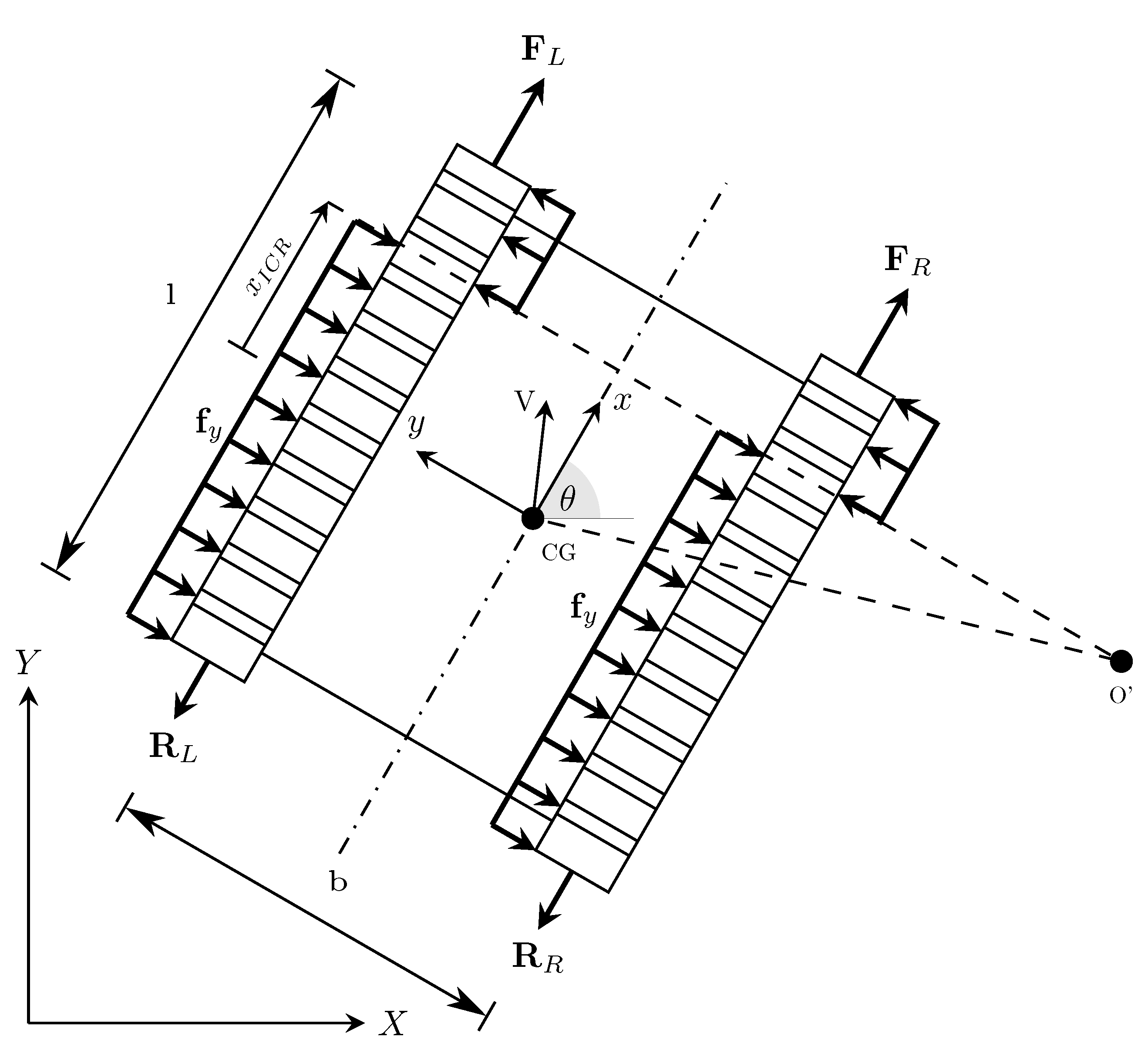
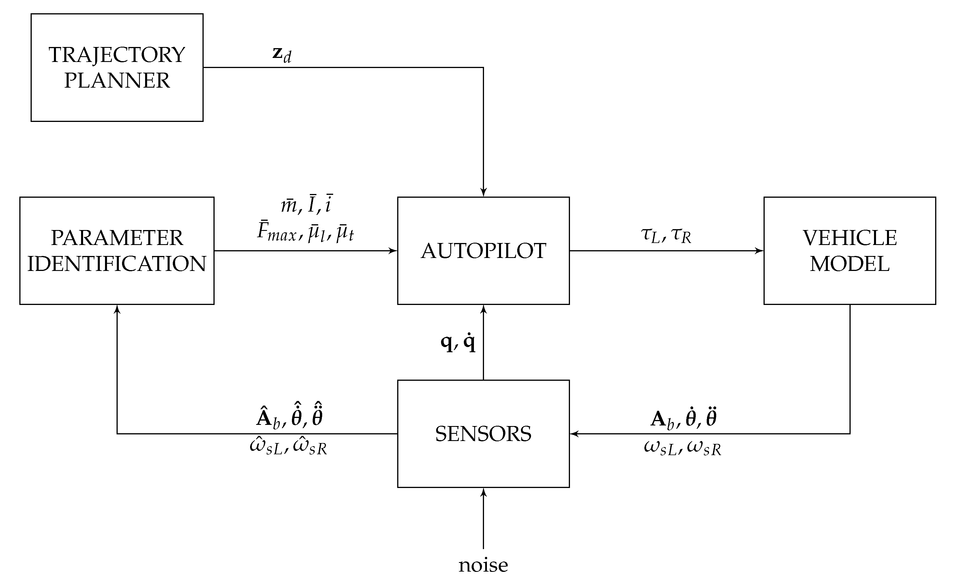
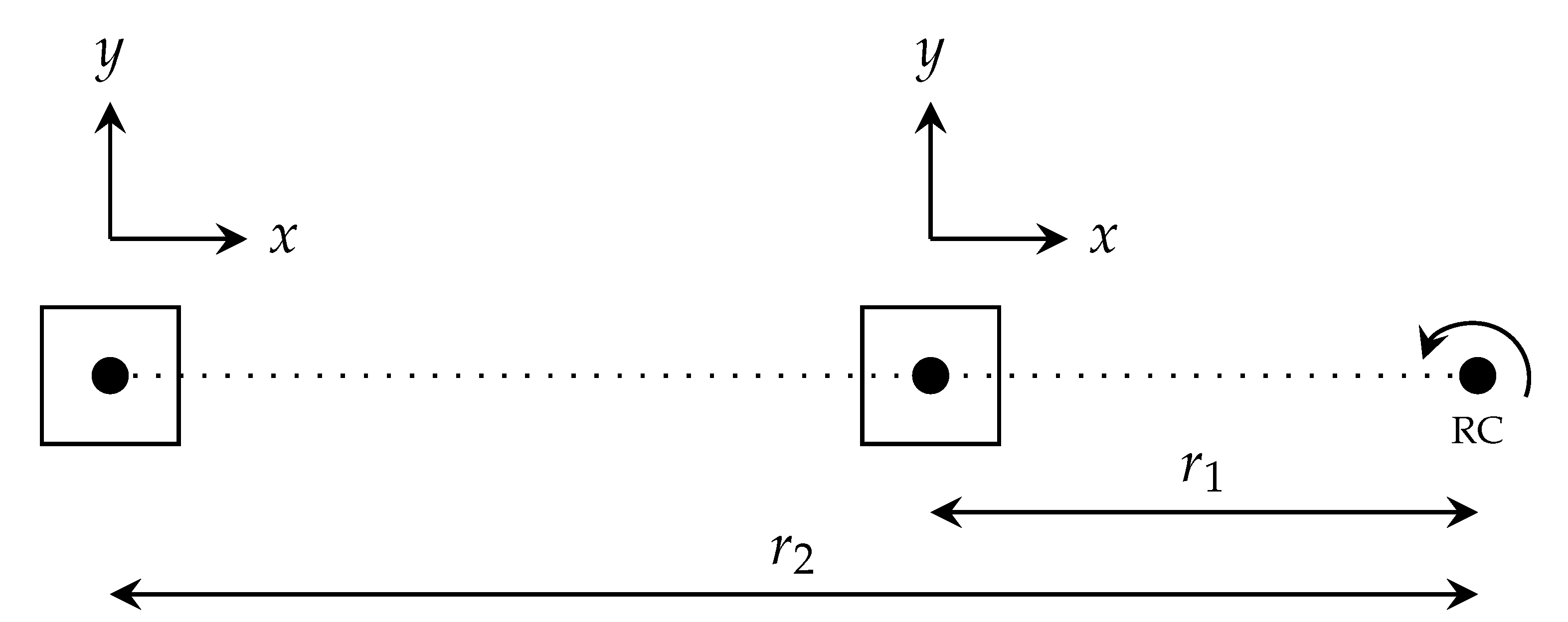
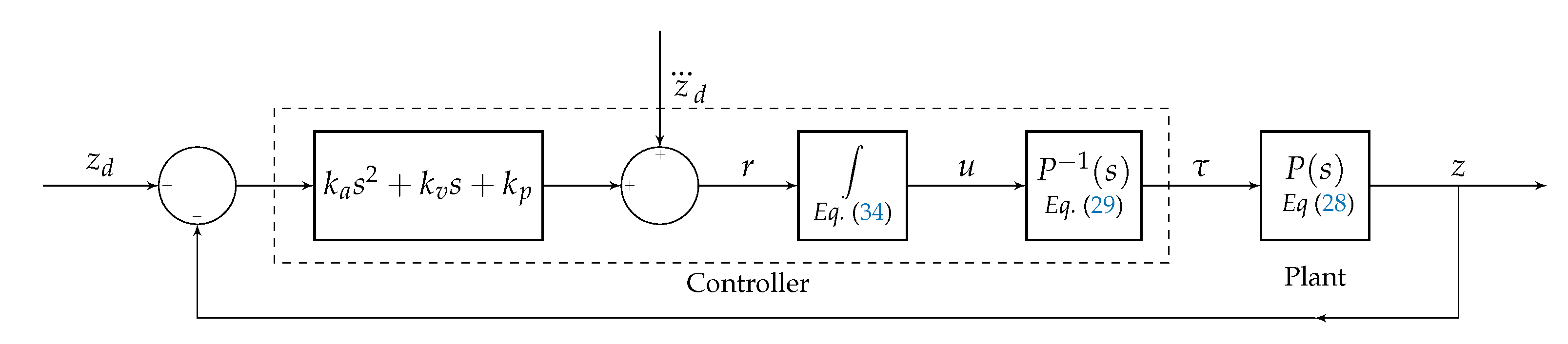
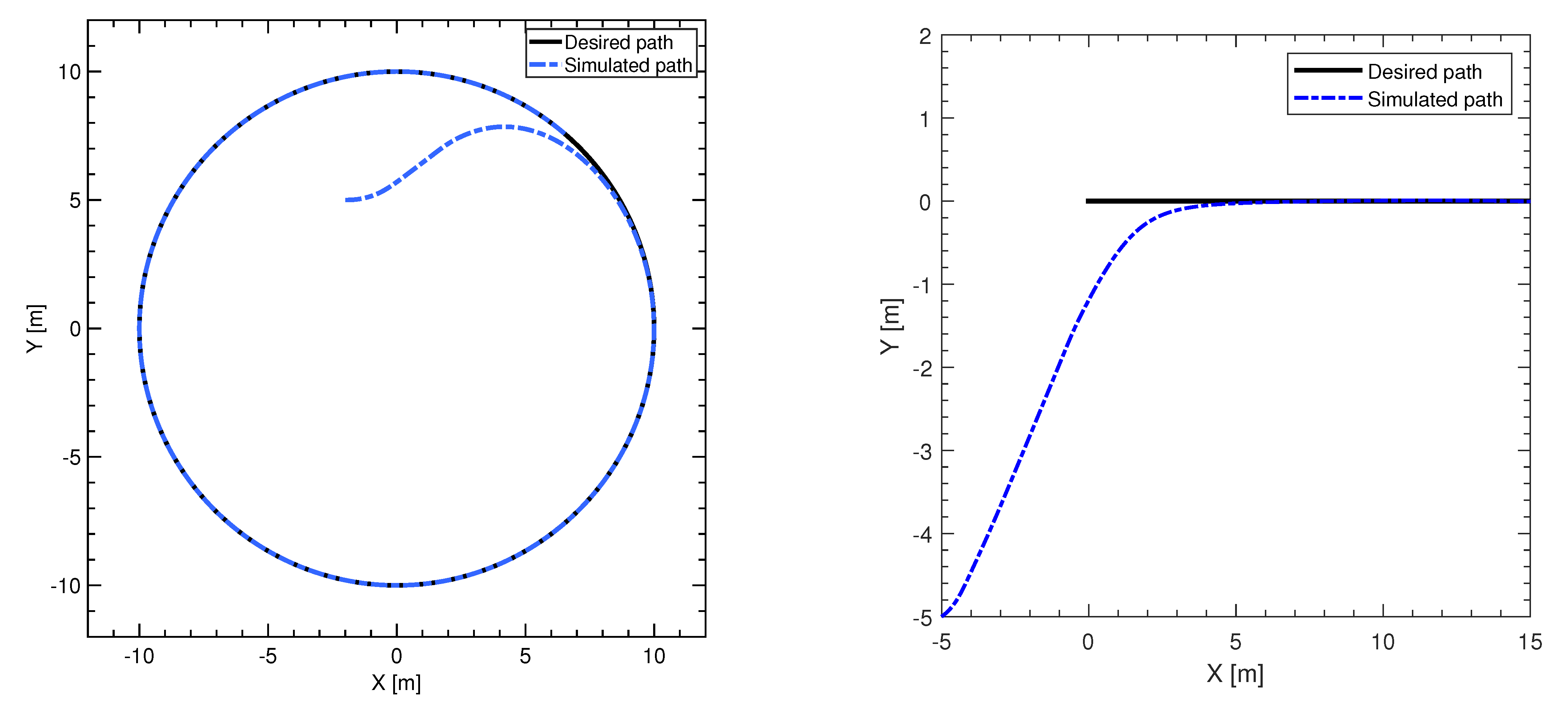
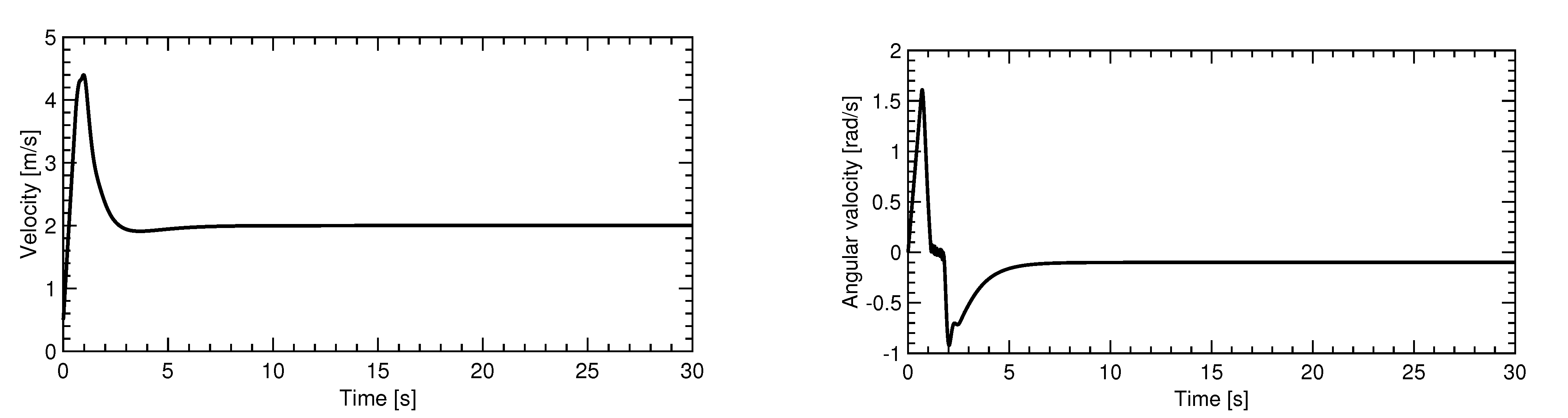
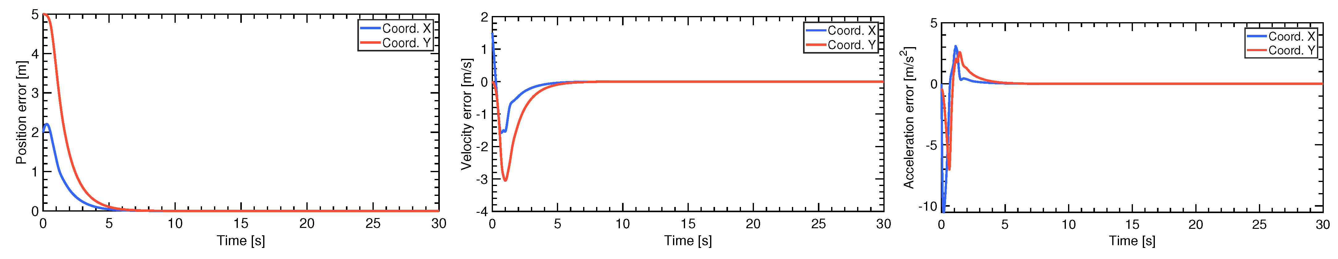
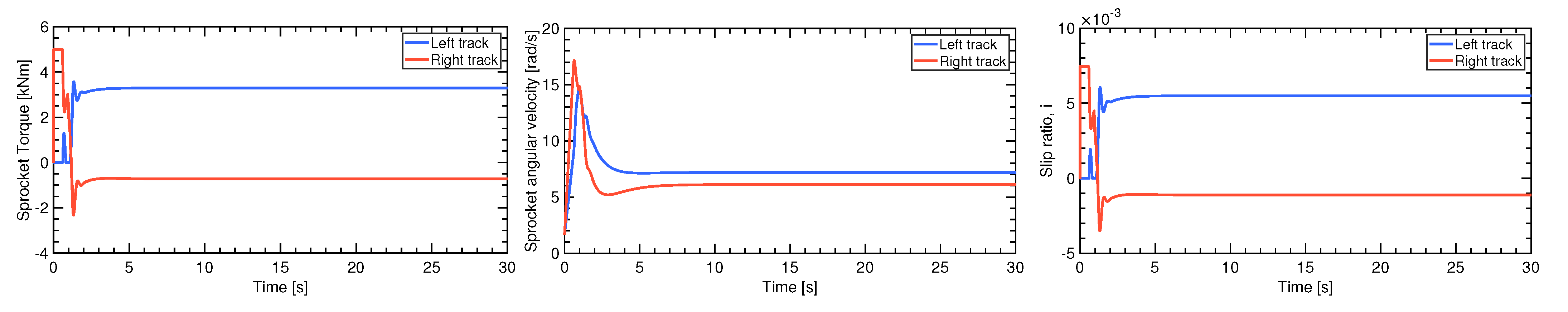
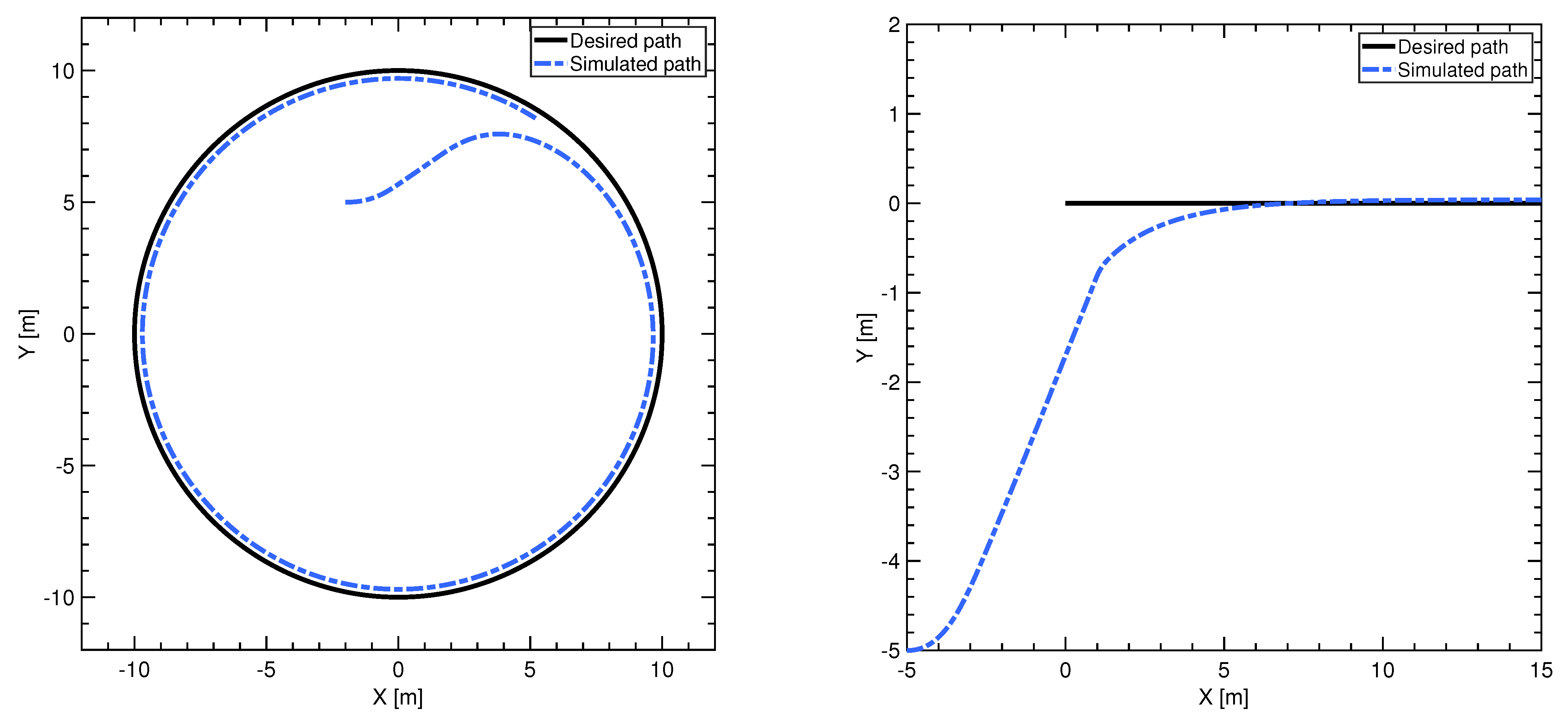
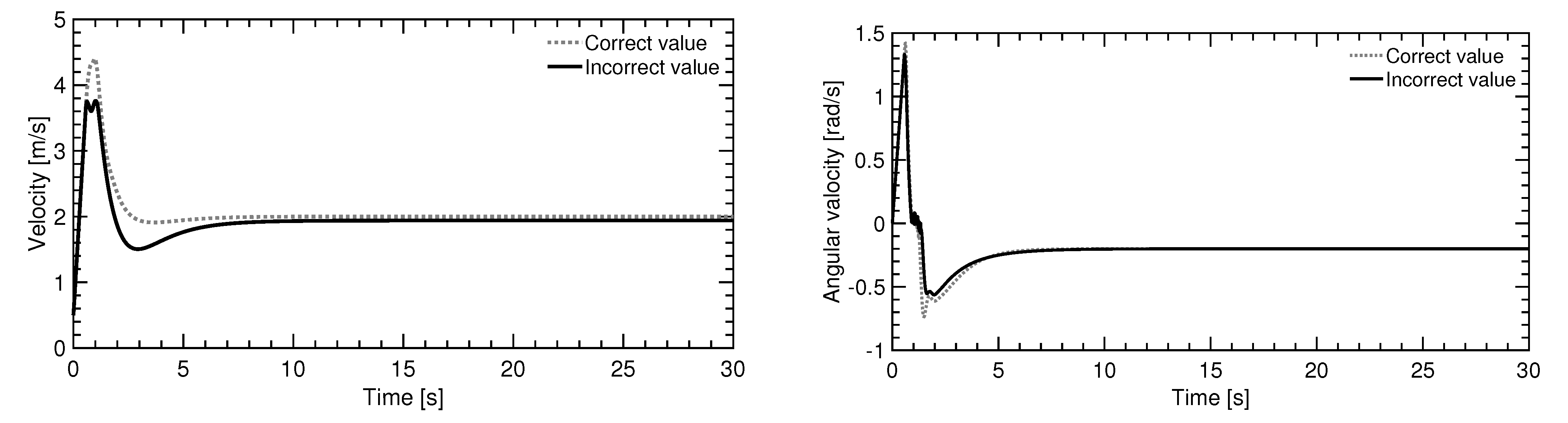
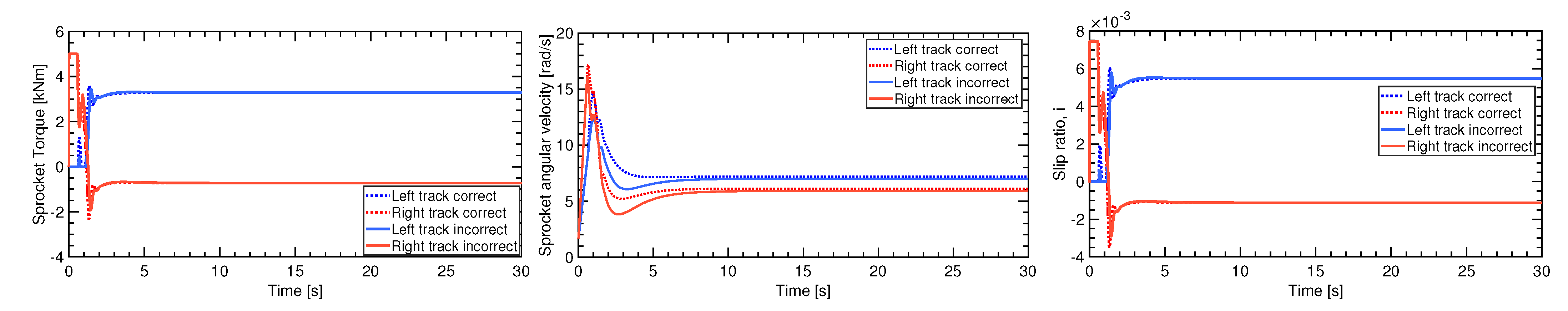
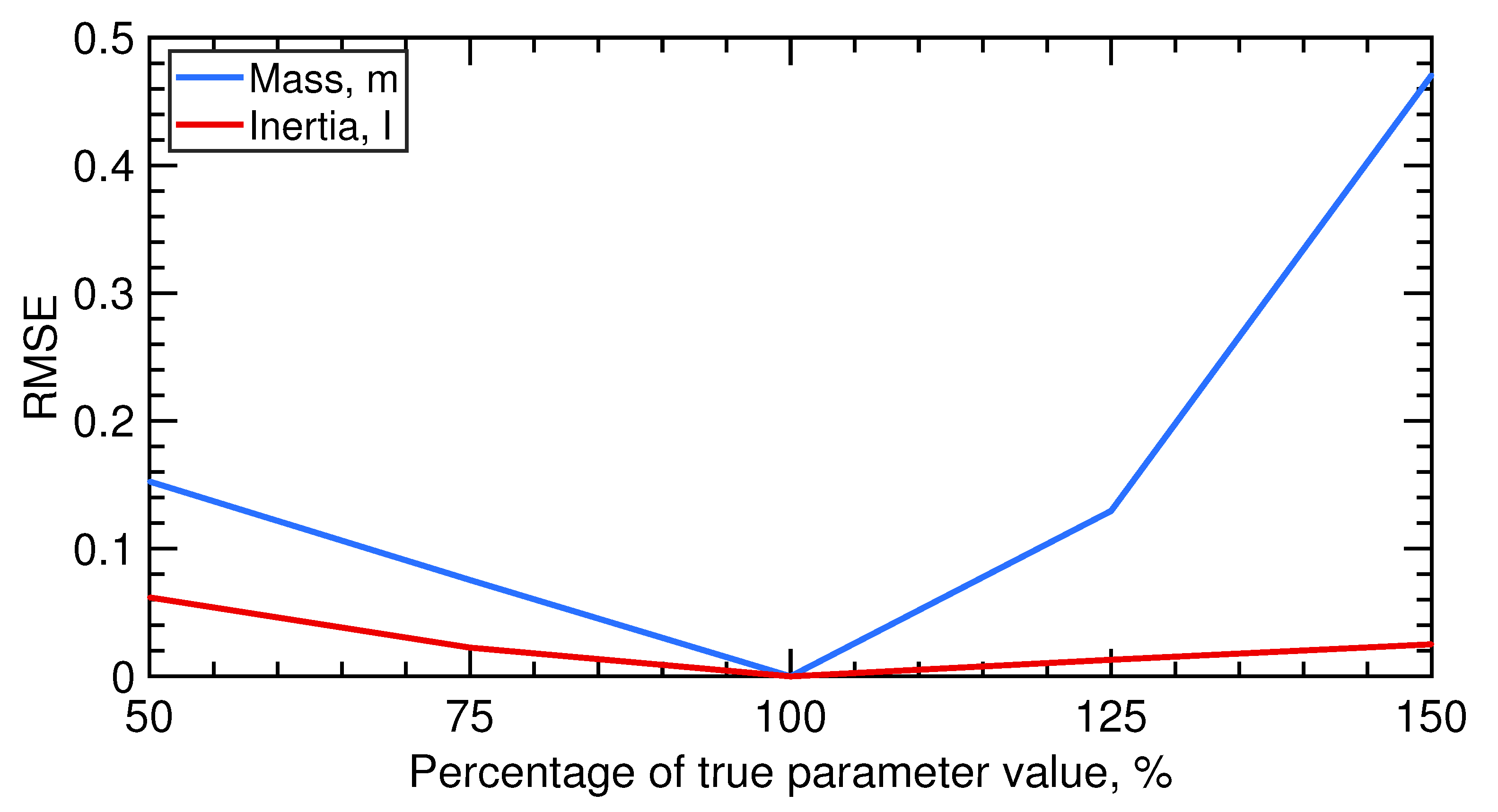
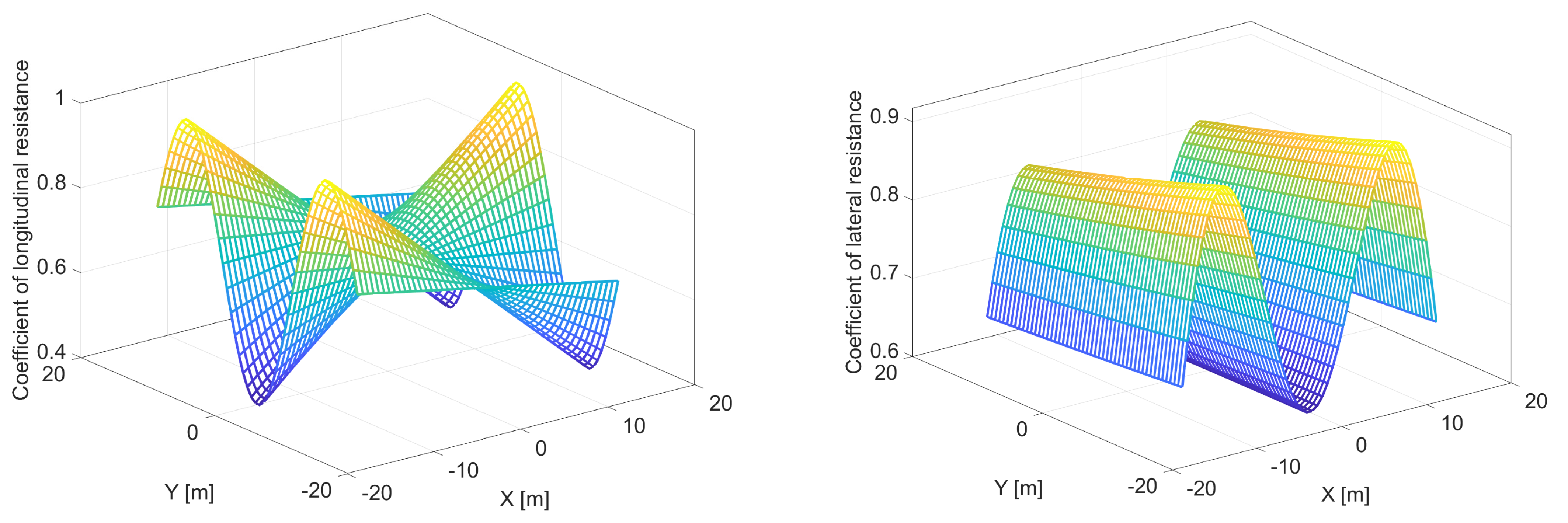
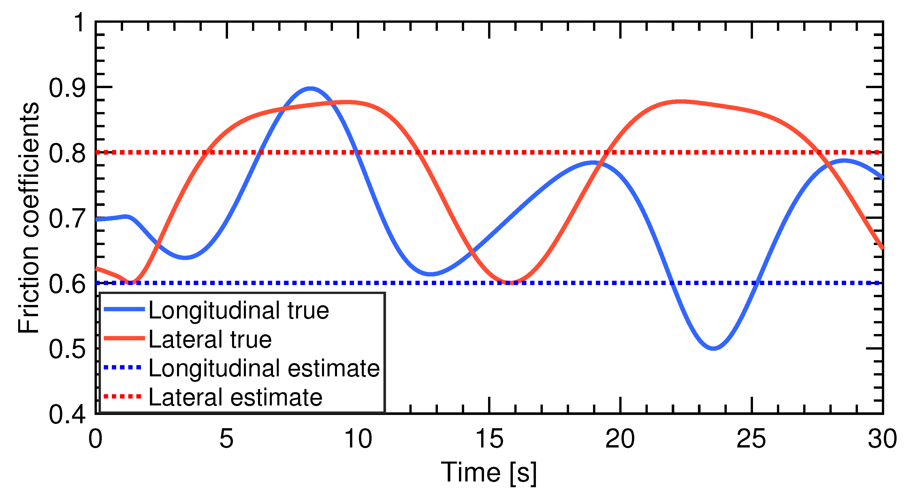
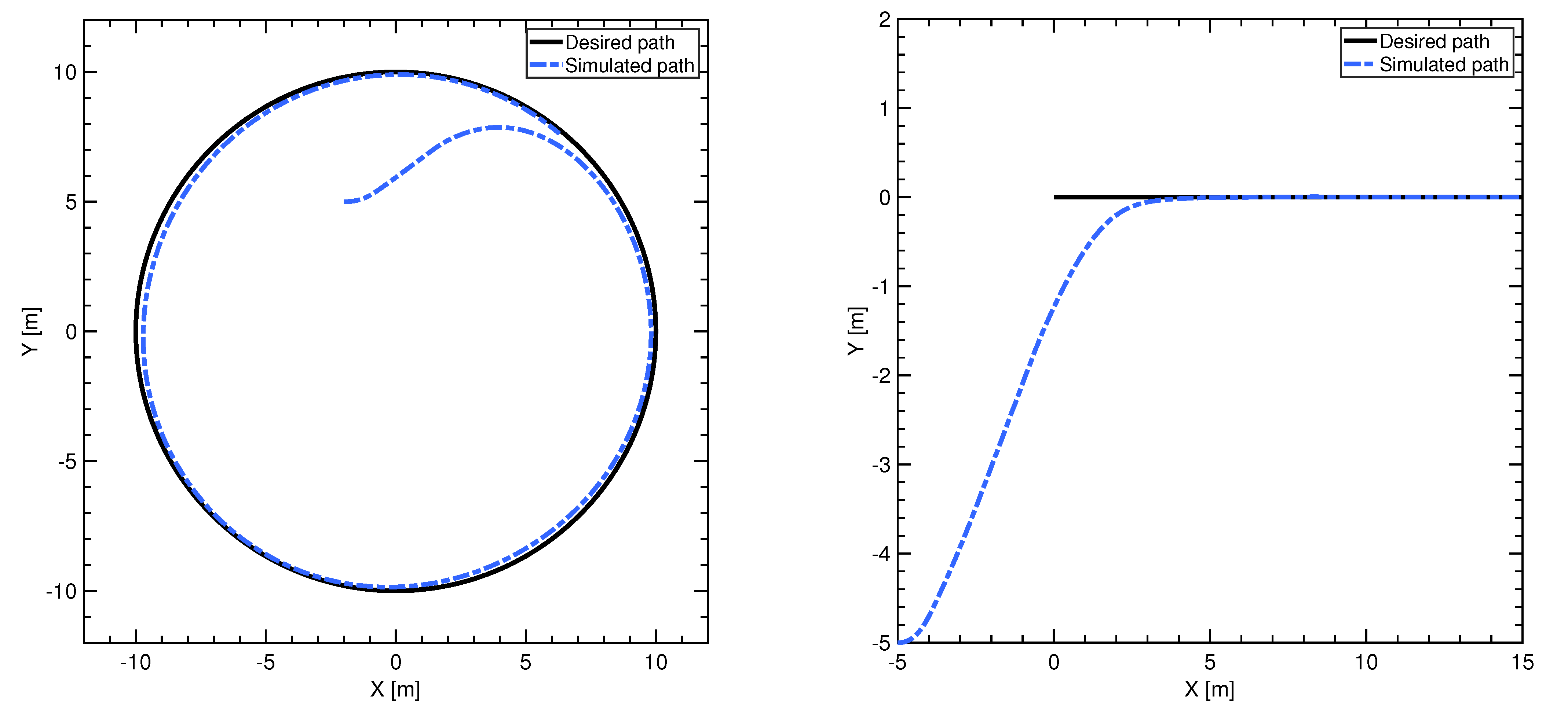
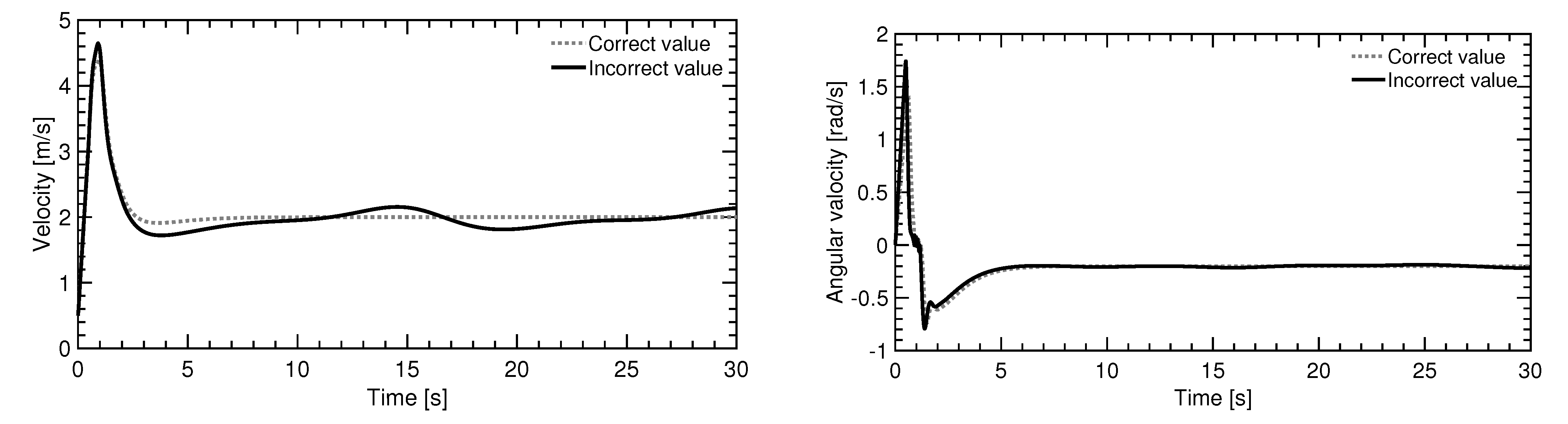
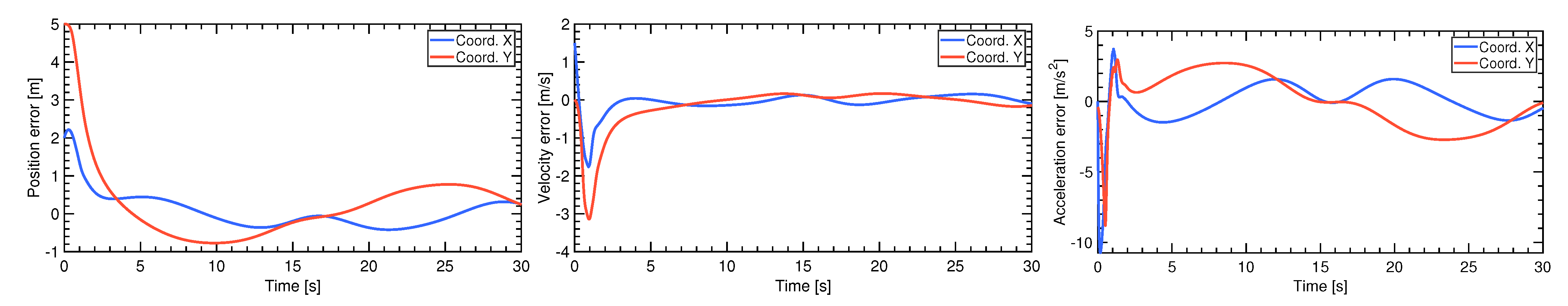
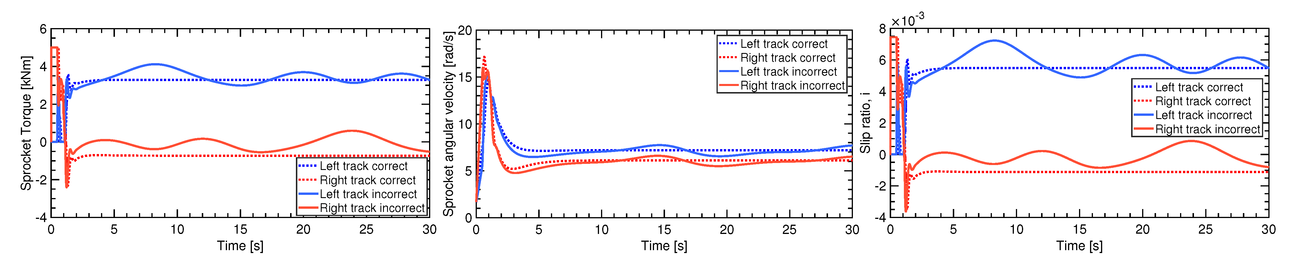
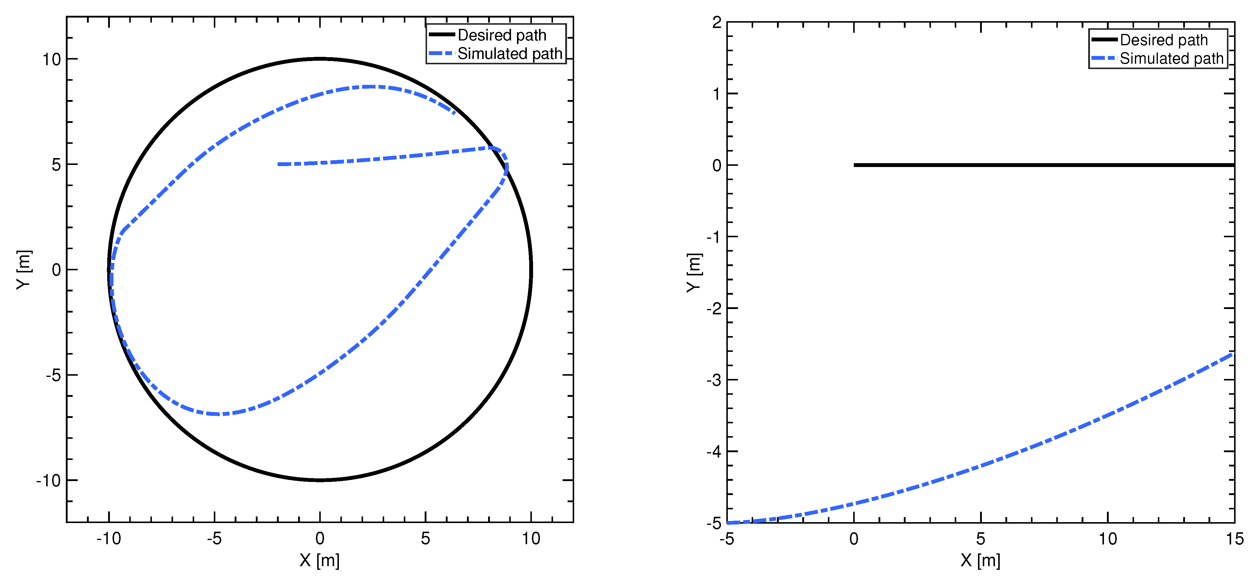
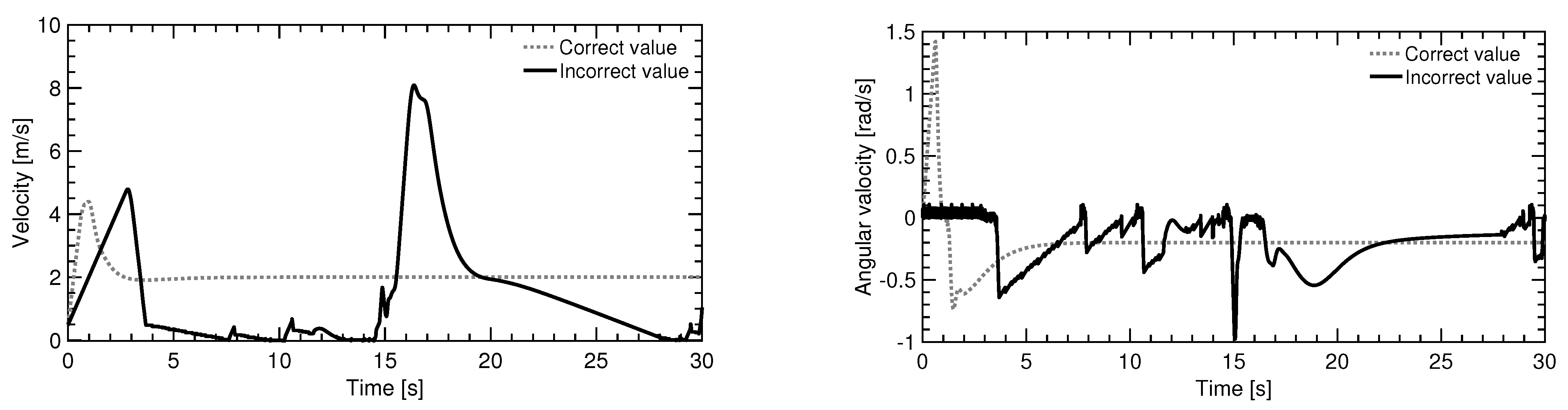
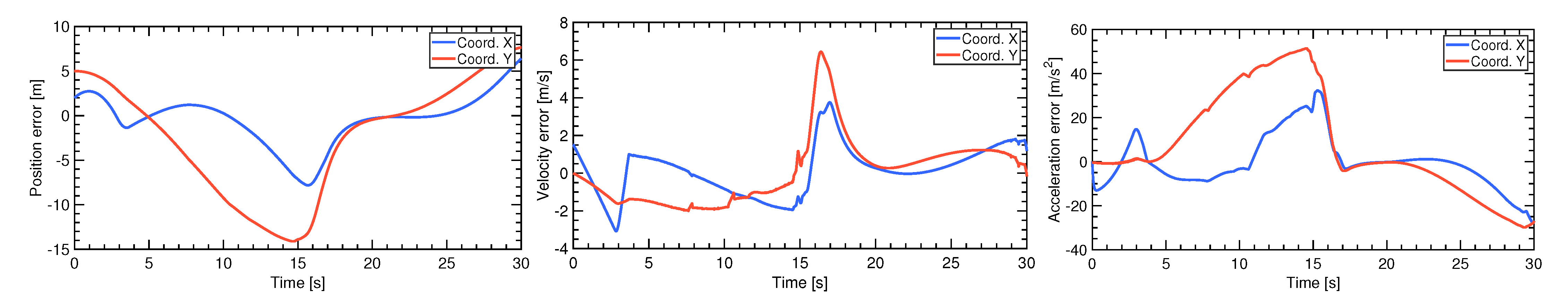
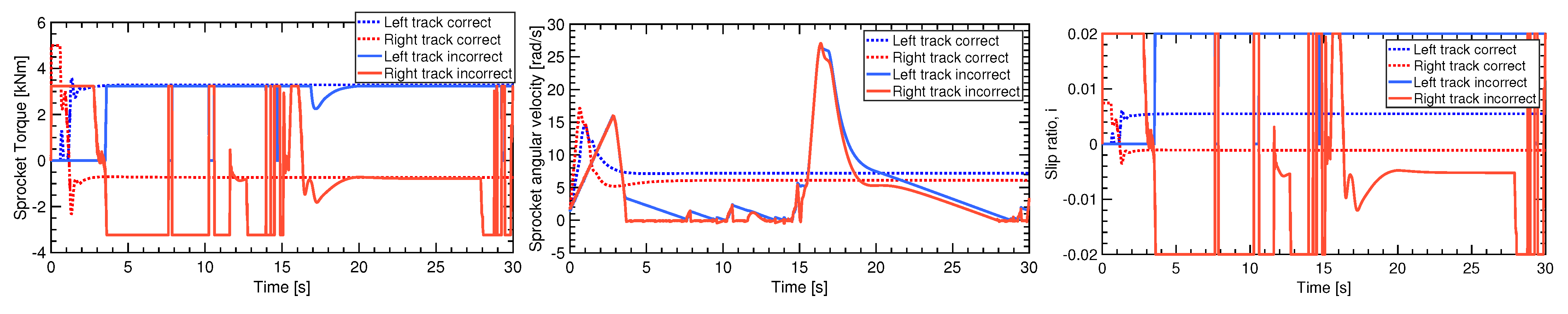
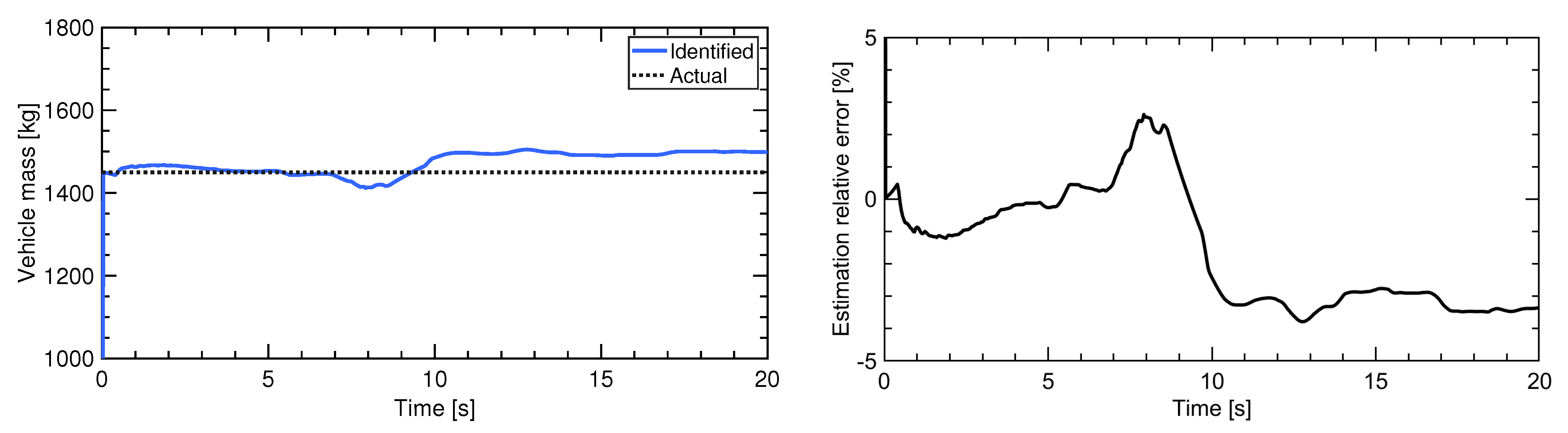
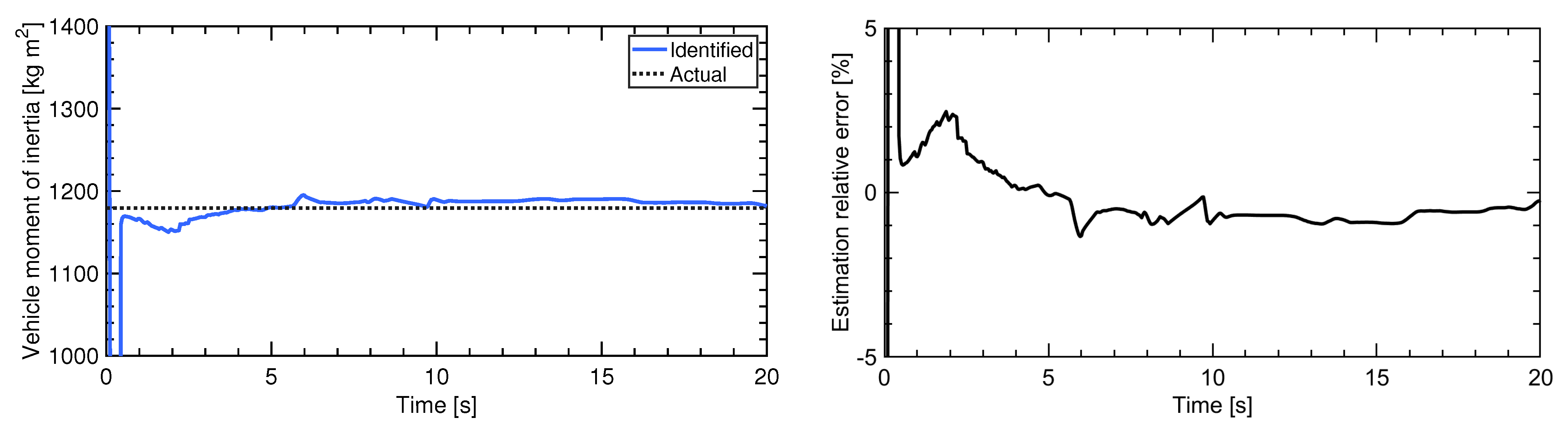
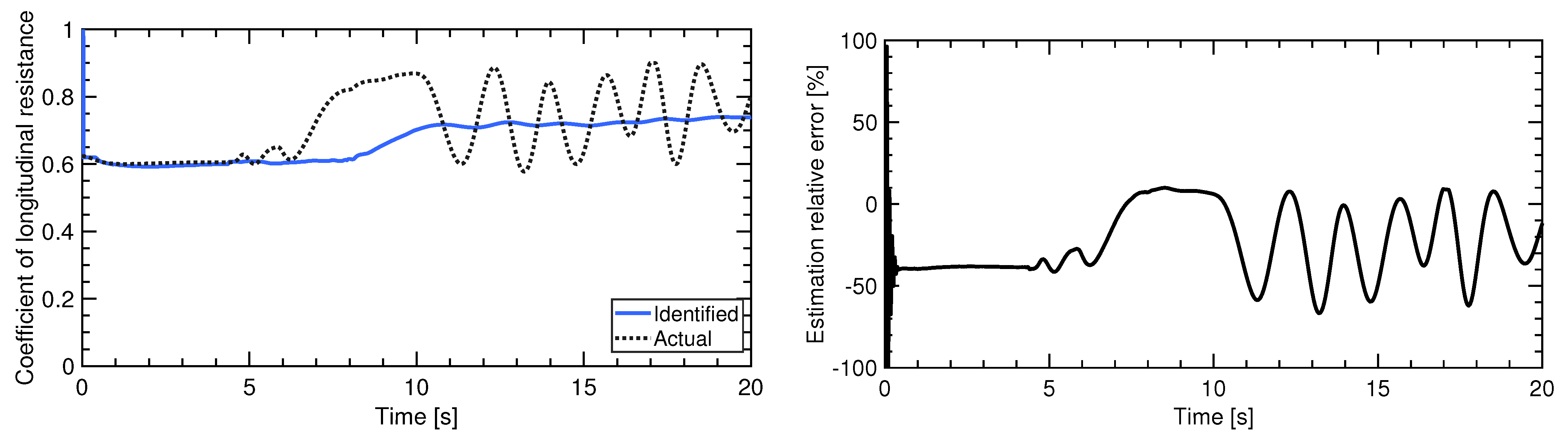
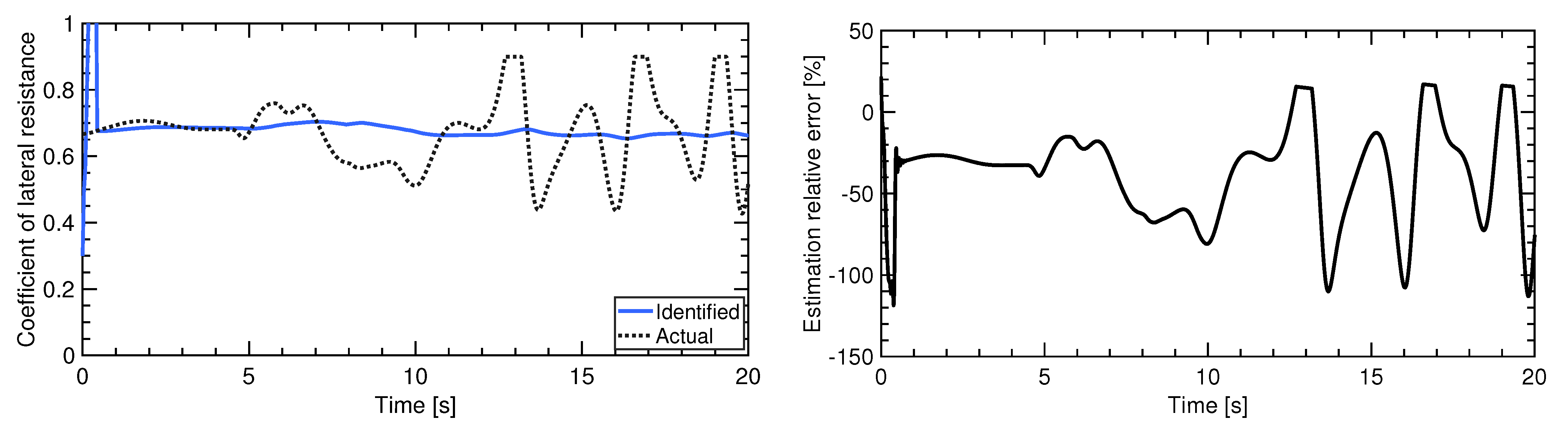
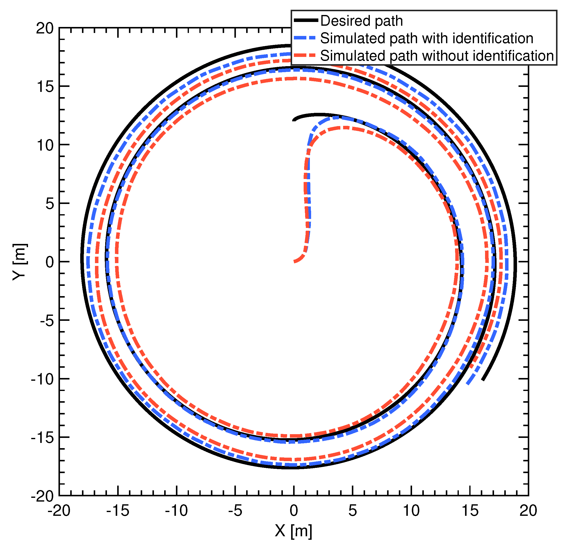
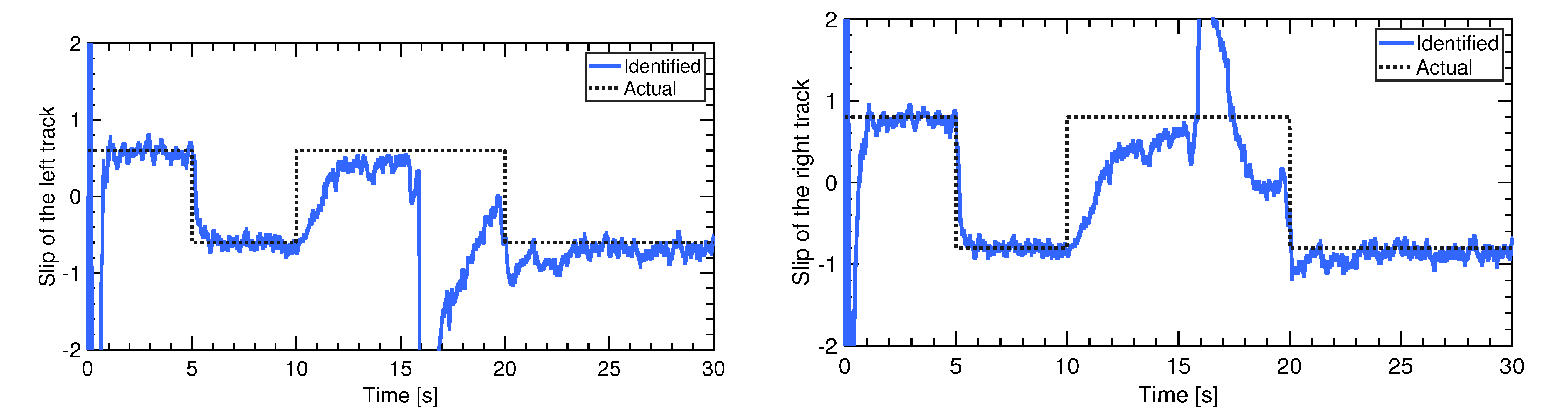
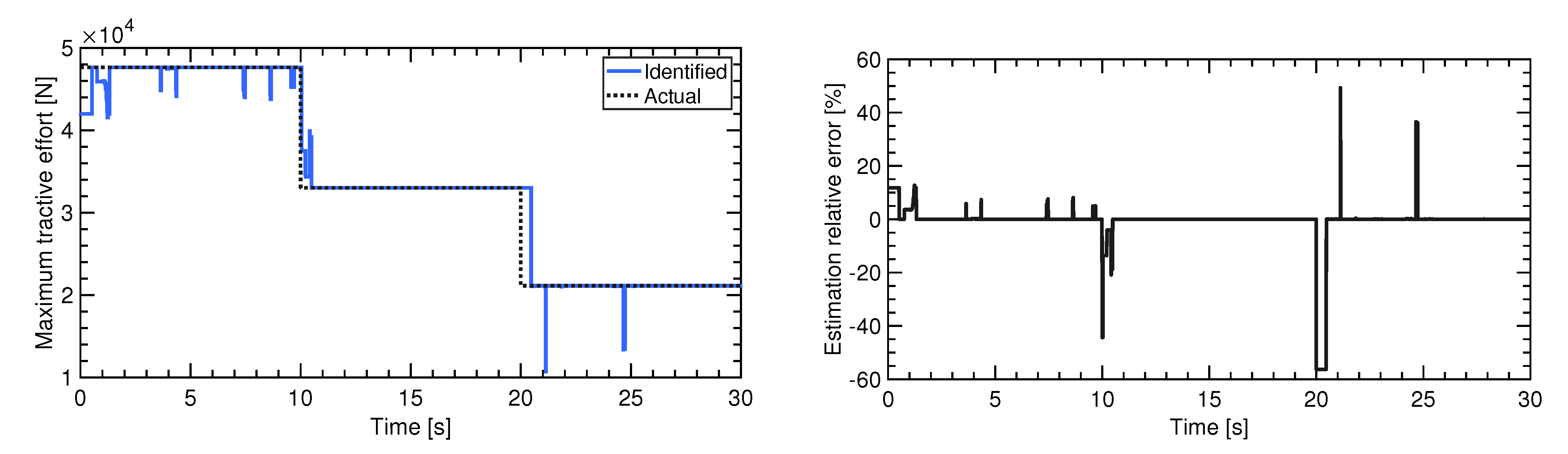
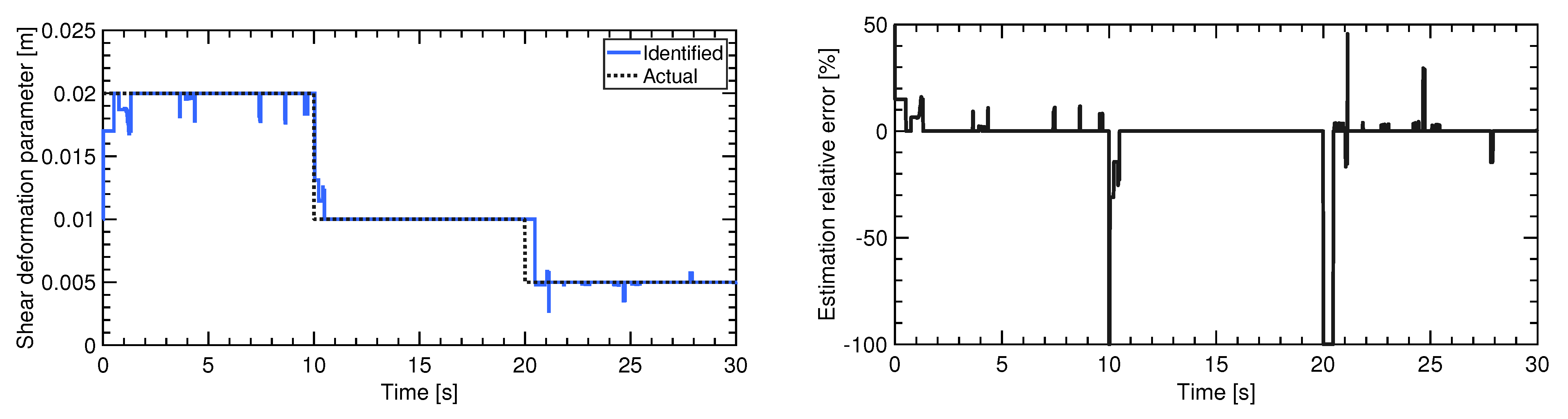
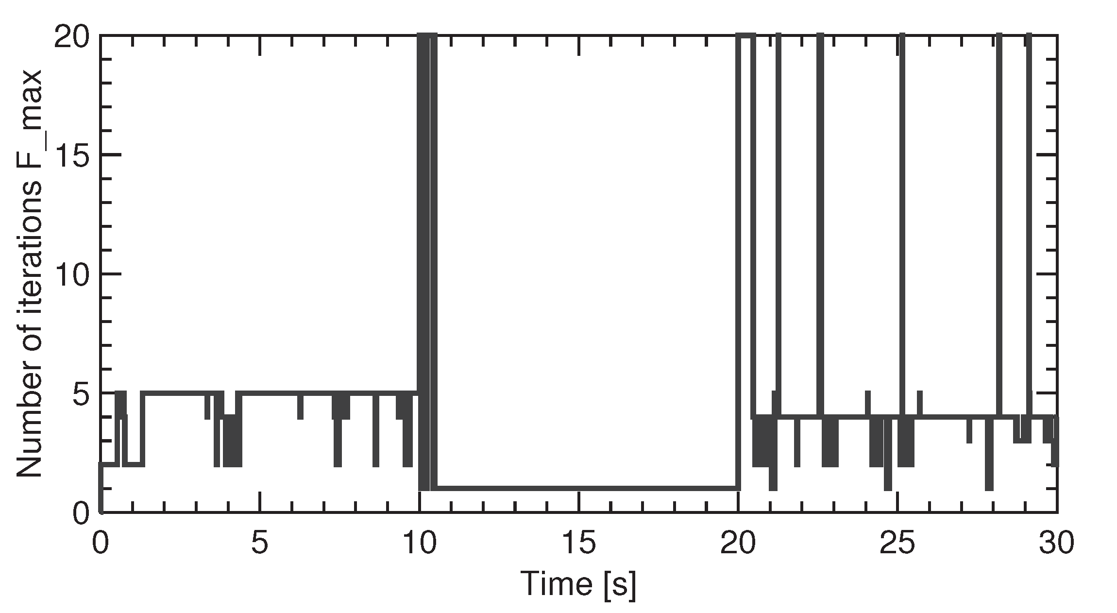
Table 1.
Vehicle parameters.
| Parameter | Value | Unit |
|---|---|---|
| Mass, m | 1450 | kg |
| Inertia, I | 1180 | kg · m |
| Tread, b | m | |
| Track width, w | m | |
| Track contact length, l | 2 | m |
| Sprocket radius, r | m | |
| Gear ratio, n |
Table 2.
Soil parameters for heavy clay [5].
Table 2.
Soil parameters for heavy clay [5].
| Parameter | Value | Unit |
|---|---|---|
| Cohesion, c | 70 | kPa |
| Angle of internal shearing resistance, | deg | |
| Shear deformation parameter, K | m | |
| Coefficient of longitudinal resistance, | ||
| Coefficient of lateral resistance, |
Table 3.
Final values of the controller gains.
| Gain | Final Value | |
|---|---|---|
| 50 | ||
| 70 | ||
| 15 |
Publisher’s Note: MDPI stays neutral with regard to jurisdictional claims in published maps and institutional affiliations. |
© 2021 by the authors. Licensee MDPI, Basel, Switzerland. This article is an open access article distributed under the terms and conditions of the Creative Commons Attribution (CC BY) license (http://creativecommons.org/licenses/by/4.0/).
Share and Cite
MDPI and ACS Style
Strawa, N.; Ignatyev, D.I.; Zolotas, A.C.; Tsourdos, A. On-Line Learning and Updating Unmanned Tracked Vehicle Dynamics. Electronics 2021, 10, 187. https://doi.org/10.3390/electronics10020187
AMA Style
Strawa N, Ignatyev DI, Zolotas AC, Tsourdos A. On-Line Learning and Updating Unmanned Tracked Vehicle Dynamics. Electronics. 2021; 10(2):187. https://doi.org/10.3390/electronics10020187
Chicago/Turabian StyleStrawa, Natalia, Dmitry I. Ignatyev, Argyrios C. Zolotas, and Antonios Tsourdos. 2021. "On-Line Learning and Updating Unmanned Tracked Vehicle Dynamics" Electronics 10, no. 2: 187. https://doi.org/10.3390/electronics10020187
Note that from the first issue of 2016, this journal uses article numbers instead of page numbers. See further details here.