Predicting the Existence and Prevalence of the US Water Quality Trading Markets

BenDor, Todd K.; Branham, Jordan; Timmerman, Dylan; Madsen, Becca

doi:10.3390/w13020185

Open AccessFeature PaperArticle

Predicting the Existence and Prevalence of the US Water Quality Trading Markets

¹

Department of City and Regional Planning, University of North Carolina at Chapel Hill, Chapel Hill, NC 27599, USA

²

Matson Consulting, Lexington, SC 29072, USA

³

Electric Power Research Institute (EPRI), Palo Alto, CA 94304, USA

^*

Author to whom correspondence should be addressed.

Water 2021, 13(2), 185; https://doi.org/10.3390/w13020185

Submission received: 1 December 2020 / Revised: 30 December 2020 / Accepted: 31 December 2020 / Published: 14 January 2021

(This article belongs to the Special Issue Cross-Sector Green Infrastructure for Improving Urban Storm Water Quality)

Download

Browse Figures

Versions Notes

Abstract

:

Water quality trading (WQT) programs aim to efficiently reduce pollution through market-based incentives. However, WQT performance is uneven; while several programs have found frequent use, many experience operational barriers and low trading activity. What factors are associated with WQT existence, prevalence, and operational stage? In this paper, we present and analyze the most complete database of WQT programs in the United States (147 programs/policies), detailing market designs, trading mechanisms, traded pollutants, and segmented geographies in 355 distinct markets. We use hurdle models (joint binary and count regressions) to evaluate markets in concert with demographic, political, and environmental covariates. We find that only one half of markets become operational, new market establishment has declined since 2013, and market existence and prevalence has nuanced relationships with local political ideology, urban infrastructure, waterway and waterbody extents, regulated environmental impacts, and historic waterway impairment. Our findings suggest opportunities for better projecting program need and targeting program funding.

Keywords:

water quality trading; environmental markets; market-based mechanism; environmental policy; ecosystem service markets; ecosystem services

1. Introduction

Recent years have seen a ground-swell of bipartisan support for market-based environmental policies, such as water quality trading (WQT; e.g., [1,2,3,4]) programs. Much of this interest has been driven by the political appeal and technology forcing potential of WQT and other environmental markets [5]. Early work by Breetz et al. [6] and Morgan and Wolverton [7] determined that, as far back as 2004, there were dozens of proposed or operating programs, more than doubling the numbers from only a few years before [8]. More recently, Bennett et al. [9] documented nearly 100 water quality trading programs, with many of them created with funding support from the US Environmental Protection Agency (USEPA; [10]). While the prevalence of WQT markets has grown, the scholarly literature on WQT has exploded over the last decade. A search of “water quality trading” on Google Scholar reveals more than 4000 publications on the topic, with ~2100 of them published since 2010.

However, the performance of WQT markets is uneven [11,12,13]; while several WQT markets have seen frequent trades, many experience operational barriers and exhibit low trading activity [14,15,16,17]. Unfortunately, while a variety of work has offered deep insight into the factors that drive the success and failures of specific WQT markets (e.g., [7,18]), there are still efforts actively aimed at predicting where markets are likely to emerge and operate successfully [9,19,20]. What are the broader environmental, political, demographic, and economic factors associated with WQT market existence and abundance? Where do these markets tend to be established and where does trading actually occur (as opposed to pilot studies and other markets that exist only “on paper”)?

In this paper, we offer a comprehensive evaluation of environmental, economic, and social factors associated with the existence and implementation of WQT. Based on previous work (e.g., [21,22]), we hypothesize that demographic change—articulated as higher populations, population densities, and population increases—may create political pressure for these markets. We also hypothesize positive relationships between WQT and income (e.g., [23,24]), liberal political ideology [25], hydrological network extent and precipitation (as a proxy for nonpoint source runoff), permitted aquatic ecosystem damage [26], and the prevalence and intensity of agricultural [27] and urban activities (e.g., [28]). Finally, given the extensive recent attention to water quality as public policy issue (e.g., [29]), we seek to test whether waterbody impairment—both current and historic—and subsequent, localized regulations are associated with WQT market creation.

To test these hypotheses, we create a dataset comprising a census of WQT programs in the United States (as of 2018), delineating programs into separate markets based on their geographies, trading mechanisms, market designs, and the pollutant traded. We analyze this dataset using hurdle models (a joint binary logistic and negative binomial count model) to jointly understand the existence and prevalence of WQT markets, including markets of any type (markets of all stages) and markets that have achieved operational stages. In this paper, we seek to identify the environmental, economic, and social variables that predict (or are associated with) market establishment and prevalence. We do not seek to comprehensively address the complex and in-depth qualitative mechanisms that inhibit or accelerate WQT markets, which has been the subject of excellent prior studies by authors such Shabman and Stephenson [18] and van Maasakkers [30].

We begin with a discussion of our data collection and analytical methods, detailing the reasoning driving the construction of our models. We then present our results that new market establishment has declined through 2013–2018 and that market existence and prevalence has nuanced relationships with local political ideology, waterway and waterbody extents, regulated environmental impacts, and historic waterway impairment. We also find a positive relationship with the extent of historic waterway impairment and a negative relationship with road network density. Contrary to expectations, we generally find weak, indeterminate relationships between the extents of impaired (i.e., highly polluted) and regulated waterways, as well as measures of urban density (i.e., population, population change, and density). Finally, we offer discussion and conclusions suggesting opportunities for better projecting market need and targeting program funding.

2. Materials and Methods

2.1. WQT Market Data Collection

To census WQT markets, we set out to collect market information in two phases. Phase 1 involved compiling and augmenting data in existing program lists, including a list created as part of the USEPA’s EnviroAtlas project [9] and another list created by the Electric Power Research Institute [31]. These lists, which, in many cases, overlapped in their included markets, were themselves the result of literature reviews of previous market lists created by groups such as the Environmental Trading Network [32,33], the US Department of Agriculture’s (USDA) Office of Environmental markets, and the Willamette Partnership (e.g., [34]).

To complete our Phase 1 search, we augmented these lists, looking for market-specific resources and recording relevant information (detailed in the next subsection) into a market database. We merged all available market data, performing additional searches (and sometimes contacting program officials) to determine which markets were applicable to this project and to find additional information, as needed. In the course of researching known markets, we would frequently find references to additional markets that were not already in our market database. Those markets became the foundation of our Phase 2 list. It is important to note that—given the breadth of markets considered in this study—we were unable to thoroughly interrogate the true nature of market activity in the tradition of Van Maasakkers [30] or others, who might seek to differentiate markets based on their complexity and tenure (e.g., differentiating long-term trading vs. one-time trades in bilateral markets).

Once all relevant, previously known markets were compiled into a single database, we began adding to our Phase 2 list (markets not previously compiled), conducting an additional survey of the literature using Google Scholar and the ProQuest academic database, searching all materials available using the terms “water quality trading,” “nutrient trading,” “WQT,” “phosphorus trading,” and “nitrogen trading.” The results of the first 20 pages (800 total hits) were investigated in detail for references to markets not already included in “Phase 1” of our market database. Through conversations and reviews with WQT experts, additional markets were also brought to our attention.

Like the markets in Phase I, we set out to identify important characteristics of each market using a combination of information provided in the literature, searches of market and related-government websites, and supplementary follow-up conversations with officials involved with the markets. In total, we found an additional 222 markets as a result of the Phase 2 search, many of which were markets that we disaggregated from within broader WQT programs identified in Phase I sources (e.g., the Alpine Cheese and Walnut Creek phosphorous trading programs, which are both administered by the Holmes County (Ohio) Soil and Water Conservation District; [9,35]).

2.2. Database Design

There were several detailed aspects of WQT arrangements that we sought to capture in our market database. These included market names, types, and stages of development, as well as enabling authorities and whether these authorities established a stormwater program.

We structured this market database hierarchically; a given, named WQT program can include distinct and multiple markets. We considered markets within a program to be distinct if they traded different pollutants (e.g., a nitrogen market and a phosphorus market), used a different market structures (detailed below), or traded within distinct geographic areas (i.e., separate spatial trading areas). For each individual WQT market, we collected information about the market’s geography and extent (i.e., spatial trading area), pollutant traded, market structure, the types of buyers and sellers (private or public), trading ratios (rarely available), and whether the market was active at the end of 2015 (when our search began).

We must note that geographic trading areas do not necessarily equate to the “service areas” in offset markets, which is defined as the spatial zone of allowable transactions between impacts and a given offset site [36]. Service area data were often not available, and so we only include geographic trading areas as a way to identify and distinguish the entirety of the area covered by a given WQT market.

2.3. Program and Market Typologies

We rely strongly on previous work that has endeavored to comprehensively describe program and market characteristics, including market structure, program type, transaction type, and program stage. To begin, Woodward et al. [37], defines “market structure” as the “...market’s standards for obtaining information and exchanging rights.” Our market structure typology is based on work by Morgan and Wolverton [7], who define this structure based on the rules and practices around the trading of credits between buyers and sellers within the program. Under this typology, while markets can allow for multiple market structures, they tend to fall into one of the following five categories:

Bilateral: terms of trades are negotiated directly between the buyer and seller.
Clearinghouse: an intermediary entity pays for pollution credits and then sells them to buyers.
Third party: a third-party broker is involved in identifying potential trade partners and facilitating trades (typically for bilateral negotiations).
Sole source offset: an individual entity is allowed to meet requirements for a single site by reducing pollutant load in another area.
Not established: no market structure was defined in the creation of the market.

Next, we also set out to classify the regulatory environment in which a program operates, which we broadly refer to as “program type.” This descriptor concerns the program’s trading practices and the regulatory requirements that the program is designed to meet. We consider four program types, drawing on definitions established by the USEPA’s water quality trading evaluation study [10]:

Cap-and-trade: a pollution limit is put in place (therefore creating a “closed” market), typically by governments or other market manager. Pollution discharge allocations are allocated to participants, who then trade these allocations with each other [38].
Case-by-case: all trades must be reviewed and preapproved by an overseeing authority.
Open market: a system of rules is put in place and participants can trade freely among themselves without preapproval from regulators or a mandatory program-wide cap.
Not established: no specific trading mechanisms are articulated during program creation.

Third, we sought to describe the type of entities engaging in trades, defining “transaction type” based largely on the point source (PS) or nonpoint source (NPS) nature of those participating. Therefore, we can imagine PS-PS, PS-NPS, NPS-PS, and NPS-NPS transactions. We also added two additional categories to account for government entities involved in transactions. The fifth category describes markets structured around “Payments for Ecosystem Services” (PES) arrangements, whereby governments pay private entities for beneficial land management activities (e.g., [39]). The sixth, and final, category includes in-lieu fee programs (ILF), in which private entities pay governments in lieu of offsetting their regulated impacts [40].

Finally, we sought to identify each market’s stage of development; how far along did the market go towards becoming operational? A previous effort by Morgan and Wolverton [41] classified WQT activities into four categories (not rigorously defined): “on-going offset/trading programs,” “one-time offset agreements,” “state and regional trading policies,” and “other projects and recent proposals.” Unfortunately, two barriers leave us unable to draw directly on this framework for defining WQT market stage. First, while an agreement may be made once, subsequent trades may occur multiple times (which is difficult to track and document), blurring the line between an “on-going trading program” and a “one-time offset agreement.” Second, “other projects and recent proposals,” aggregates together a whole variety of nuanced market stages; Morgan and Wolverton [41] go on to describe (without specifically delineating) WQT projects as “pilot studies,” “trading proposals,” “case studies,” “trading considered,” and “trading simulations/trading plans/trading authorized” (distinctions within this final category are unclear).

After collecting aforementioned data on markets and their current (as of 2018) conditions, we built on Morgan and Wolverton’s [41] framework to inductively classify each market as shown in Table 1. We note that several states have created enabling policies for WQT programs, some of which also establish operating markets (which we merge with other operational markets into Stage 5 in Table 1). However, those policies that focus only on enabling other markets are not included on the development scale.

2.4. Covariate Data

Our analysis seeks to identify the factors associated with WQT market existence and prevalence. A variety of economic and environmental literature has suggested that the presence of certain factors may increase or decrease demand for WQT market structures (e.g., [19,42]). We hypothesize that WQT efforts are reactions to current or historic pollution levels [43], and are more likely occur in areas with extensive agricultural activity [44], urbanization [28], environmental impacts and permitting (which may result from infrastructure impacts, regardless of setting; [26]), allied environmental market activity (e.g., wetland and stream mitigation activity; [19,26]), and hydrological regimes that are generally conducive to markets (e.g., experience extreme rain events and possess large river networks and/or water bodies). We also must consider the political and demographic characteristics of areas with markets, including the role of income and political affiliation, which significant work has demonstrated is aligned with enactment and enforcement of environmental policy and the local and state levels [25,45,46,47]. Table 2 details the data and data sources we use to operationalize each of these factors.

2.4.1. Ideology and Income Factors

The (often positive) relationships between income and environmental performance (and enactment of environmental policies) have been a topic of extensive study within environmental economics (e.g., the environmental Kuznets curve discussed by Dinda; [23]) and management (e.g., [24]). We draw on household median income data from the US Census’s American Community Survey (ACS; [48]).

Likewise, a variety of studies have noted the strong role of political ideology in determining environmental policy enactment [25,49,50]. We hope to determine if, and how, dominant political beliefs are correlated with WQT efforts, especially in light of a long history of bipartisan enthusiasm for more laissez-faire, market-based approaches to environmental protection [1,2]. While early support of WQT and environmental markets, generally, emerged under Republican Party leadership (see [3]), it remains unclear whether that national level support materialized at the local level through market establishment and operation.

We must highlight that we are not testing a direct causal connection between local level political ideology and WQT existence and prevalence. WQT programs are not the product of referenda in which local populations vote on their development. Nor are they electoral issues (e.g., ballot proposals) in places where they have been implemented. However, while much more complex dynamics may be at play in the establishment of any given WQT market (including institutional network effects and policy learning at a variety of governmental levels; [30]), we nevertheless hypothesize a positive relationship between the WQT activity and dominant political ideologies among residents that would support stronger environmental regulations (i.e., more liberal populations).

The relative political conservatism or liberalism of political parties can be highly dynamic and difficult to rectify over time (i.e., the Republican Party does not equate to political conservatism; [51]). In spite of early Republican Party support for WQT, American political conservatism has a long history of opposition to water quality regulations [25,45,46,47], including regulatory implementations of WQT. Therefore, we operationalize “political ideology” using Tausanovitch and Warshaw’s [52] regression-generated estimates of the average policy preferences of residents at county level. Their index places conservatism and liberalism on a continuous scale ranging from −1 (staunchly liberal) to +1 (staunchly conservative). A large number of studies have used this index for local-level political and policy analyses on topics ranging from autonomous vehicle preparedness [53] to rezoning decisions [54].

2.4.2. Agricultural and Population Density Factors

A long literature details the emergence of WQT as a response to widespread reticence to regulate and measure agricultural pollution (e.g., [37,38]). Much of this work points towards the potential of WQT to act as mechanism to incentivize agricultural nonpoint source (NPS) polluters to reduce their nutrient loading and provide less expensive options for point sources (PS; e.g., wastewater treatment plants) to reduce nutrient discharges [57]. We include a number of agricultural measures in our analysis, with the aim of disentangling the roles of intensity (accounting for both row crop and livestock agriculture: percentage of land in crop production, percentage fertilized cropland, mean number of cows and pigs per 100 ha of farmland), production and economic importance (mean value of agricultural products sold per farm), and land use patterns (average farm size; to distinguish areas with large numbers of small farms from those with small numbers of large-tract agriculture [43]). We hypothesize that, as areas with intensive row crop agriculture and livestock production are often leading nutrient sources [58,59], they will also be the frequent home to WQT markets. However, many large, animal-intensive farms are regulated as point sources [60] and may be participants in conservation programs (e.g., USDA Environmental Quality Incentives Program (EQIP); [61]) that could offset the need for WQT.

Similar to the role of agriculture in prompting WQT market establishment, we can note the increasing attention given to urban water pollution and subsequent management efforts [17,62]. Efforts to create urban WQT programs—primarily framed as “stormwater management” or “stormwater crediting”—have increased in recent years [63]. To highlight this trend, we use a proxy measurement of the extent of urban infrastructure, drawing on the density of street networks, as compiled by the USEPA’s Smart Location Database [55]. We also include measures of population, and population change, and density as standard measures of settlement size, change, and intensity, respectively. We draw on data from the US Census Bureau and acquired via Social Explorer [64,65], which uses the Longitudinal Tract Data Base (LTDB; [66]) to geospatially rectify past US population data into modern geographic boundaries.

2.4.3. Environmental Impacts and Markets

The US Clean Water Act of 1972 is the primary, federal legislation covering waterways and waterbodies in the United States (33 U.S.C. 1251 et seq.). A vast set of caselaw controls the physical and geographic reach of the law, with a recent interpretation cementing expanding jurisdiction to groundwater pollution (140 S. Ct. 1462; 2019). The law is multifaceted and creates numerous permitting programs for managing a variety of impacts to water and water quality.

We theorize that these permitted impacts, which are frequently associated with increased activity and water stress [67], will be positively associated with WQT program existence and prevalence. First, under the Act’s National Pollution Discharge Elimination System (NPDES) program (Section 402 of the Act; 33 U.S.C. 1342), permits are granted to regulated point source polluters (e.g., wastewater treatment plants and factories). Second, Section 404 of the Act (33 U.S.C. 1344)—and Section 10 of the similarly managed US Rivers and Harbors Act of 1899 (33 U.S.C. 403)—creates a permitting system for regulating impacts from development on federally regulated wetlands and streams [28]. We likewise theorize a positive relationship with efforts to offset damage from Section 404/10 through wetland and stream mitigation banks [68].

Data for federal point source permitting is available through the USEPA’s [69] NPDES permitting database, while data for Clean Water Act Section 10/404 permitting is available from the US Army Corps of Engineers’ (USACE) [70] ORM2 database. Finally, wetland and stream mitigation banking offset data are available through the USACE RIBITS database [71,72].

2.4.4. Hydrologic Factors

We would hypothesize that water quality and the stringency of water quality regulations would be the primary drivers of WQT programs [38]. However, while a huge number of localized water quality datasets are available through resources such as the National Water Quality Data Portal [73] and the USGS National Water Information System [74], these data are not uniform—in either their collection or spatial distribution—across the United States. While some researchers (e.g., [75,76,77]) have, regardless, endeavored to assemble these databases for use in national-scale analyses, these collection efforts cannot overcome the lack of uniformity in direct measurements at the scale and breadth needed for this study. Instead, we test for relationships between water quality and WQT markets using a variety of land use, regulatory, and historic indicators of waterway impairment as proxies.

First, while intensive agriculture is a dominant contributor to nutrient loading in streams [44], and therefore possibly to the existence of WQT, we need to control for the role of rainfall intensity. While more precipitation may lead to more nonpoint runoff (e.g., higher nutrients) in areas with extensive agriculture, it can also lead to greater instream dilution, potentially negating some nutrient loading problems. We account for the impacts of extreme rain events using a measure of the maximum total monthly precipitation experienced at the county-level from 1980 to 2014 (maximum monthly precipitation; [56]).

BenDor et al.’s [26] analysis of wetland and stream mitigation banking activity found that the total amount of wetland area—the resource that was impacted and restored in wetland mitigation markets (a closely aligned environmental market to WQT)—was the major driver of bank establishment. Similarly, we hypothesize that WQT activity will be correlated with greater extents of river networks and other waterbodies (e.g., ponds and lakes).

WQT often involves ecological restoration as an offset mechanism [37]. Likewise, WQT is typically geared towards addressing waterbody impairment, which is typically designated by the USEPA and state water quality agencies on the Clean Water Act’s Section 303(d) list of impaired and threatened waters [78]. Some waters may experience total maximum daily load (TMDL) limitations and subsequent regulations imposed by state water quality regulators in response to these impairment designations [79]. Therefore, we also hypothesize that the extents of impairment and subsequent regulatory interventions (e.g., [80]) in an area’s waterways and waterbodies will be positive indicators of WQT activity. We rely on geospatial data detailing hydrological extents from the National Hydrography dataset [81]. The USEPA’s [82] WATERS database also offers comprehensive data on the extents of regulated (i.e., TMDL regulations) and impaired waters, including currently and historically impaired (2002) waters.

2.5. Data Processing and Sampling

WQT markets have nonuniform geographies (e.g., locally defined eco-regions, state-defined soil and water conservation districts, municipal boundaries, and watersheds) and vary substantially in their spatial scale. In terms of watershed scales, which are defined in the United States using the US Geological Survey’s nested Hydrological Unit Code (HUC) framework (see [83]), markets range in size from an entire, multistate river basin (a 2-digit basin or “HUC-2”; e.g., the World Resource Institute’s Mississippi River Basin Nutrient Trading program; [84]) to a municipality or a single, small watershed (e.g., the Shepherd Creek Stormwater Crediting program, covering a partial HUC-14 watershed (~200 ha) in the State of Ohio; [85]).

While we can use these data to understand the complex and varied geographies of areas establishing markets, we do not have the (nonexistent) geographies of those areas not establishing markets (i.e., counterfactuals). Therefore, we need to create a standardized geographic unit of analysis that can be uniformly—and without bias—used to distinguish between areas with, and without, markets. This unit of analysis must be uniformly available across the United States, and it must be small enough to allow fine-grained spatial analysis that disentangle areas with and without markets.

We initially considered the US counties and small-scale watersheds, such as the universe of HUC-12 watersheds, as potential units. We concluded, however, that use of watershed boundaries would require excessive summarizing and aggregating of demographic, agricultural, ideological, and economic data, which are natively measured at the scale of administrative boundaries (e.g., tracts and counties), eliminating spatial variation and analysis power. Following recent work by Keiser and Shapiro [75], who study how grant money allocated by the Clean Water Act has influenced water quality across the United States, we selected the US Census Tracts (“tracts”; 2010 boundaries) as our unit of analysis. While tracts are not units of government (we address this below), they allow us to incorporate a wide range of demographic and economic explanatory variables at their native resolutions. Moreover, tracts are subdivisions of the US counties, and therefore, do not suffer from spatial disaggregation or aggregation problems for county level data.

All data was summarized to the tract level, using spatial intersection queries from the sf package [86] in the R statistical software (v3.6.0), which was used for all data management and analysis [87]. Most explanatory variables were summarized to the tract level; others—riverine networks, waterbodies, and permitting information—were summarized to tracts using spatial intersections. WQT markets were assigned to tracts by calculating the amount of overlap between each WQT market and Census tract, and then using a 50% threshold to categorize whether the tract possessed a WQT market. Appendix A offers more details on transformations and outlier removal, and Appendix B discusses sensitivity analysis in merging tracts and WQT market geographies.

There is an important issue that we must confront in using relatively small geographic analysis units. In assigning WQT markets to census tracts, we must account for potential for statistical bias and endogeneity problems that arise as a result of the spatial clustering of contiguous tracts within a market. When a single WQT market spans many contiguous tracts (and many markets do), then clustering effects of those tracts can artificially bias standard error estimates (see [88]). This is an inherent problem with using a small geographic unit of analysis and would occur with any geographic unit of analysis smaller than the majority of markets (e.g., counties).

To eliminate this effect, we take a simple, state-stratified random sample of Census tracts in each State; this sample must be large enough to still include enough tracts for our analysis (we do not want to drop too much of our data), but small enough to minimize the likelihood and impacts of contiguous tract clustering in the sample. Therefore, we base our analysis on a 10% sample of tracts (n = 6940 tracts; stratified by each state that has at least one WQT market), a rate that ensures a low probability that clustered tracts can bias our analysis (i.e., we are very unlikely to sample a large number of observations from a single market).

Environmental impacts (i.e., permitting) and hydrologic processes (riverine networks and waterbodies) can occur at a range of watershed scales, from small (HUC-12) to very large (HUC-2). While our unit of analysis is the US Census tract, which allows for an exploration a variety of demographic factors, looking at hydrologic and environmental permitting variables in isolation within individual tracts may not reflect the environmental realities that might inform WQT program creation. That is, a given tract’s propensity to have a WQT program within its boundaries may be the result of hydrological and environmental permitting factors surrounding it (beyond the tract boundaries).

We evaluated the sensitivity of our models to summarizations of hydrologic and environmental permitting variables at different scales, including the Census tract, the surrounding HUC-8 watershed, and the surrounding HUC-6 basin [83]. We find that with these variables summarized to the HUC-6 and HUC-8 levels, model fit substantially improves and signals become clearer. Given the important role of whole-watershed dynamics in predicting impairment and driving WQT implementation [36,89], we present our primary findings using variables summarized to the HUC-8 level (Table 3). See Appendix C for a presentation of results with hydrologic and environmental permitting variables summarized to the tract and HUC-6 level (Table A2 and Table A3, respectively).

2.6. Hurdle Regression Modeling

We expect that there are structural differences in the relationships between predictors of the existence of a single WQT market in a tract and predictors of many WQT markets existing simultaneously. Individual factors may contribute to establishing an initial market in a tract in different ways than they may contribute to prompting additional markets. For example, Woodruff and BenDor [90] explore this issue with respect to the existence and abundance of wetland and stream mitigation sites, noting that the barriers that prevent creation of an initial site can fall after it is created, prompting additional, subsequent sites.

Therefore, we employ a “hurdle” regression model [91] to allow for an exploration of WQT market existence and abundance, simultaneously. Hurdle regressions estimate two models (via maximum likelihood; see Appendix D for more information): one describing binary outcomes (zero or one) and the other modeling counts outcomes (>1). Our hurdle model allows for differentiation between the covariates (and their coefficients) that predict the presence of a WQT market (via a binary logistic regression) and the covariates that predict additional markets (a truncated negative binomial model) in a given tract.

We apply two hurdle models to different dependent variables. First, we examine the relationship between our covariates and the presence of a WQT market in any stage, from proposed (Stage 1) to operating (Stage 5). All WQT markets are included in the count of the number of existing markets in each tract. In the second model, we repeat this procedure, but limit the dependent variable to only include operating WQT markets (Stage 5). Thus, the dependent variable in this model is classified as a “1” only if a tract has an operating WQT market, and tract-level counts only include operating markets in their total. Separating these sets of outcomes into two models allows us to explore the different relationships that mediate market existence, abundance, and operation.

3. Results

3.1. Descriptive Statistics

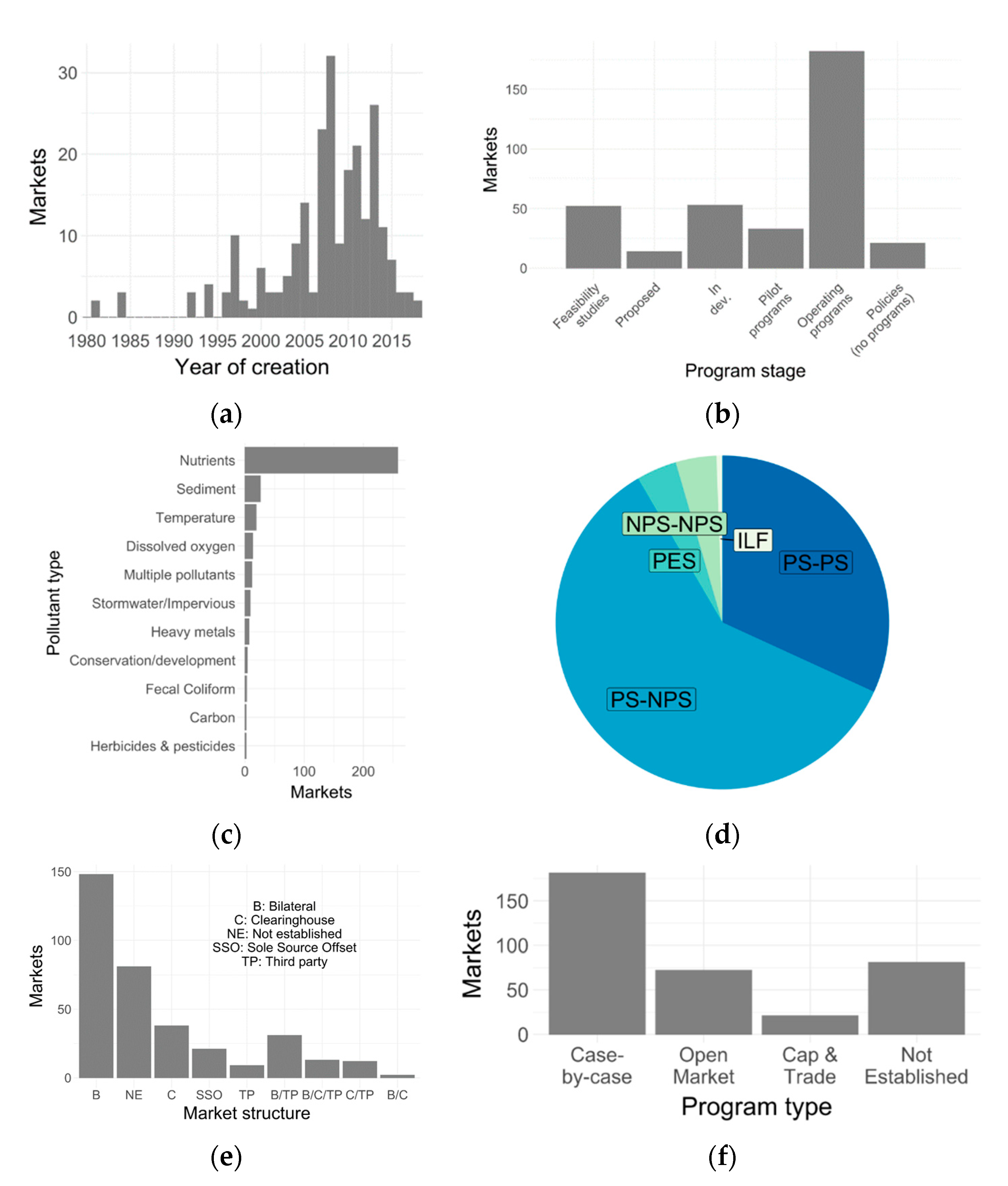
Our market collection processes yielded information on 141 WQT programs and six statewide policies. Many programs operate multiple, separate markets, each defined by distinctions in the pollutant traded, market structure, geospatial trading area, or level of implementation. We found that these 141 programs are composed of 355 individual markets, which are the focus of the remainder of our results.

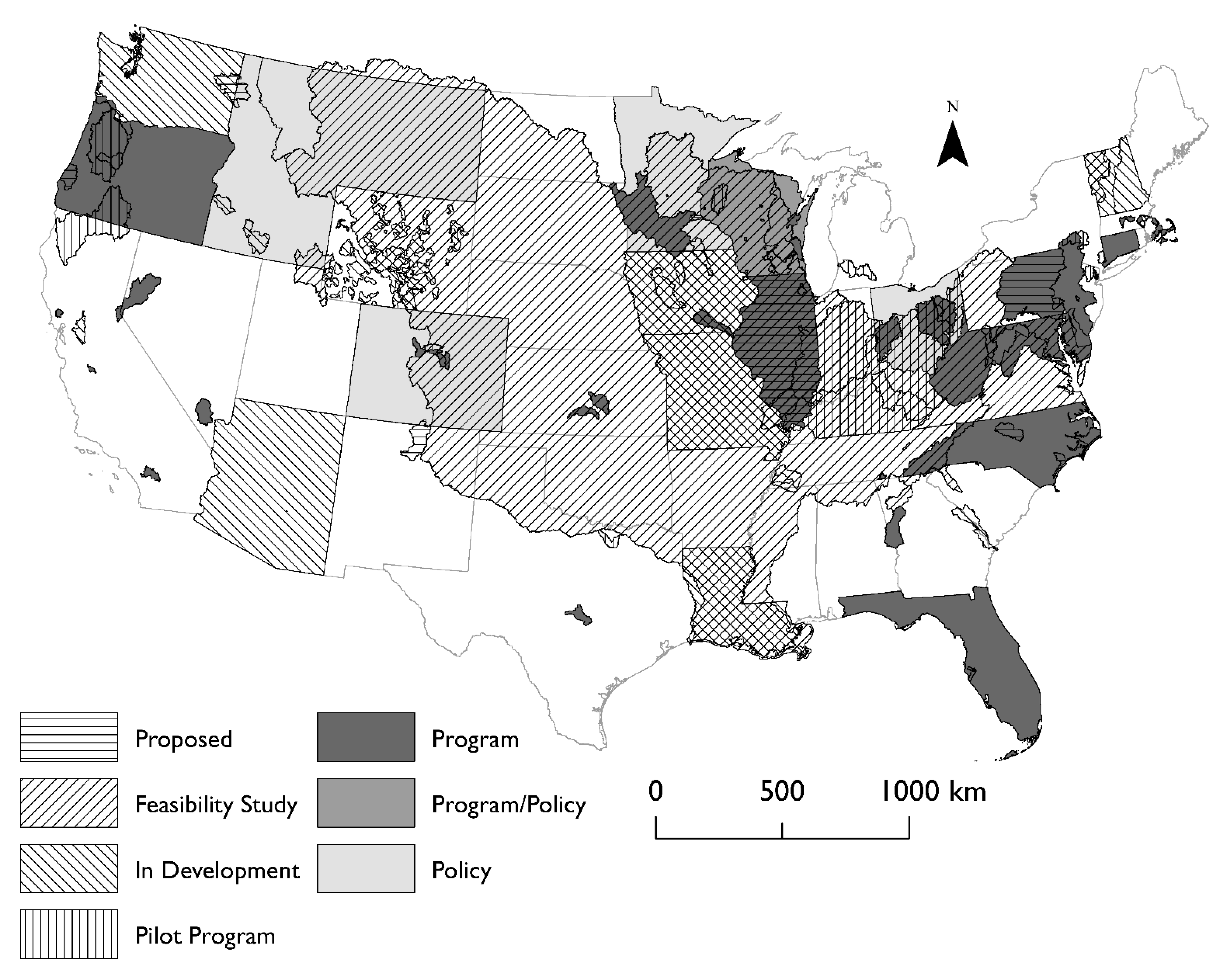
WQT markets are distributed across the country (Figure 1) with a wide variety of geographic boundaries and extents. Among them, 71.3% of markets are defined by environmental boundaries (e.g., eco-regions and watersheds) as opposed to political boundaries (e.g., municipalities, counties, and states), with 37.7% defined by one or more watershed boundaries at the HUC-8 or HUC-10 level and 21.1% defined by HUC-6 or larger river basin boundaries. Only 11 markets (3.1%; e.g., California’s Grassland Area Farmers Tradable Loads Program; [92]) have geographic boundaries that are defined by boundaries that are neither watershed nor administratively based (e.g., counties and municipalities). While a few markets are defined (at least in part) by city (2), county (1), land parcel (2), sewage treatment district (1), and water management district (3) boundaries, the remaining 26.2% of all markets are bounded by the US States.

Most WQT markets (as of 2018) were established between 2007 and 2013, with a notable slowdown in new market development since 2014. Just over half of all markets—50.1%—could be characterized as being “operational” (i.e., Stage 5) at some point in time. The majority of markets are aimed at trading nutrients (Figure 2a; i.e., nitrogen, phosphorous, ammonia, and nitrates; 72.7%), with sediment (7.3%) and temperature (5.4%) as the next most common pollutants. While many markets aimed to transact different pollutants using distinct markets, 2.8% allowed trading across different pollutants within the same market (e.g., trading nitrogen for phosphorous or across heavy metals). See Table A4 for a more specific breakdown of pollutants traded.

In terms of transaction types, nearly all markets (91.5%; PS-PS and PS-NPS) involved a point source on at least one end of trades (Figure 2b). Only 14 markets (3.9%) aim to facilitate transactions between nonpoint sources (NPS-NPS), yet 12 of those have become operational (e.g., Delaware River Basin Commission Water Quality Program [93], Maryland Nutrient Trading Program [94]). Turning to market structure, while nearly half (47.9%) of markets involved bilateral trading, market structures were never specified for nearly a quarter of all markets (22.5%). However, among markets without specified market structures, it is important to note that only two were operational (i.e., Illinois’ Metropolitan Water Reclamation District Act; Illinois Public Act 100-0341). Multiple market structures—e.g., bilateral and third-party trading—were parts of the structural design for another 16.9% of markets.

3.2. Hurdle Regressions

We found that political ideology and road network density have the clearest relationships with the presence and prevalence (count) of WQT markets across all stages of markets (Model 1; Table 3), and among operational markets, specifically (Model 2).

A one “unit” increase in political ideology score—a shift from a liberal-leaning jurisdiction (e.g., Washtenaw County, Michigan; score = −0.51) to a conservative-leaning jurisdiction (e.g., Barton County, Kansas; score = 0.51)—is associated with a 58% increase in the odds of having a program, yet a 21% decrease in the odds of having additional markets in a given tract. Political ideology’s relationship with the existence and prevalence of operational markets is less nuanced; a unit increase in conservatism is associated with a 69% decrease in the odds of finding a single operational WQT market and a 23% decrease in the number of operational markets.

Our primary measure of urban infrastructure—road network density—exhibits a marked negative relationship with the existence, prevalence, and performance of WQT markets. An increase in one roadway link per square kilometer is associated with a 12% decrease in the odds of a WQT market and a 7% decrease in the odds of additional WQT markets. Similarly, road network density is associated with a 13% decrease in the odds of an operational market and a 12% decrease in the odds of additional operational markets. We found similar, negative relationships with population and population density.

The existence of environmental impact permits tends to be associated with increased odds of WQT market existence and prevalence. Permits for point-source polluters (NPDES) have a small, positive relationship across all four models, whereas wetland and stream mitigation sites (RIBITS) have a strong, positive relationship with the existence of any WQT market and operational WQT markets. Clean Water Act Section 10/404 permits are strongly associated with increased odds of finding any stage of WQT market (32.3%), finding an operational market (22.8%), and finding multiple operational markets (4.1%).

We found that relationships with hydrological variables are mixed and ultimately unclear; increased length of riverine networks has a positive relationship with WQT market existence (of any stage), yet a negative relationship with all other outcomes, including a strongly negative impact on the odds of having an operational WQT market (31%). Conversely, increases in the area of waterbodies tends to have negative associations with the odds of having one or more WQT markets, except in the case of operational WQT markets, where it has a positive relationship (15.6%).

Surprisingly, the extents (length and area) of currently impaired waterways and waterbodies—as well as those with TMDL limitations—have limited relationships with WQT markets in any stage, yet exhibit a positive relationship with the odds of having more than one operational market. More interestingly, however, historically impaired waters (2002) exhibit a positive relationship with WQT markets in any stage yet a mixed relationship with operational markets, where increased historical impairment increases the odds of having an operational market yet decreases the odds of having multiple operational markets.

With the exception of population, which is notably negatively associated with WQT markets, tract demographic characteristics tend to exhibit weak, mixed relationships with WQT markets. Similarly (and surprisingly), agricultural characteristics and rainfall exhibit few notable relationships with WQT market existence or prevalence.

4. Discussion

4.1. Tracking Markets

Our efforts to disaggregate named “programs” into the multitude of distinct markets administered within each program has been a key aspect of database design to characterize and track WQT efforts. We have found that programs frequently establish distinct markets, which transact different pollutants between different types of entities, operate with different market structures and trading mechanisms, and trade in regulatory separated geographic areas. For example, the WQT program managed by the Delaware River Basin Commission operates 21 markets that allows for the trading of seven pollutants (total phosphorus, total nitrogen, dissolved oxygen, sediment, CBOD, ammonia, and fecal coliform) across three different program structures (PS-PS, PS-NPS, and NPS-NPS).

4.2. A Nationwide View of Markets

Our analysis demonstrates several key aspects of WQT in the United States. First, we see a dramatic slowdown in development of new markets from 2013 to 2018 (when we stopped collecting data), which is likely aligned with reductions in federal funding for market establishment [30]. While most authorities operating WQT markets are state agencies (others are almost exclusively local or regional agencies with governmental authority; see Table A5), historically, funding for these markets has not come from state agencies, but instead from two major federal funding sources: USEPA’s Targeted Watershed Program Grants [95] and the USDA’s Conservation Innovation Grants [96]. The USEPA program was retired in 2013 [97] and USDA’s program has since shifted its funding priorities towards “conservation finance and pay-for-success models, water management, and data analytics as well as for historically underserved communities” [96].

Second, our analysis partly confirms our initial hypothesis that excitement for WQT markets has prompted their creation, but often not led to their fully operational establishment. Nearly half of WQT markets have not become operational, lingering in early development stages or existing merely as “paper tigers,” without actual trading capability. In some cases, this operational lag could be the result of long time periods that sometime exist between program creation and actual trading activity (e.g., The Cherry Creek; [98]) and Dillon Reservoir [99] programs are two examples where the programs existed long before active trading).

Third, although our database documents nearly twice the number of markets as previous efforts (e.g., [9,31]), there is less diversity that we might expect among this large number of markets. For example, trading between nonpoint sources (NPS-NPS) is extremely rare, existing in only 14 markets (although 12 are operational). This is not necessarily surprising as NPS remain largely unregulated [100]. Examples of these include the Delaware River Basin Commission Water Quality Program [93] and the Maryland Nutrient Trading Program [94]. Likewise, most markets endeavor to trade nutrients in some form, and bilateral trading dominates market structures (possibly the result of transaction cost issues; e.g., [57,101,102]).

We also were somewhat surprised to find that 13 markets (five operating) appeared to allow “out-of-kind” transactions (see Zedler [103]) for discussion of in-kind vs. out-of-kind mitigation), which involve trades between pollutants (e.g., a market would allow trading phosphorous for nitrogen). While this practice is often frowned upon in other environmental markets, there may be rationales around cross-pollutant trading (and a corresponding trading that facilitates some commensuration between the pollutants) that we were unable to collect data to describe. This allowance may likewise reflect extreme efforts on the part of authorities to establish these markets in difficult contexts (e.g., situations where measurements of certain pollutants are difficult or create high transaction costs).

On a positive note, given the growing concerns over the role of nonpoint source pollution in domestic water quality issues [104,105], as well as the declining marginal returns (and increasing marginal abatement costs) from many point source reduction efforts [15,106], it was promising—although not unexpected—to see that trading among point sources and nonpoint sources (PS-NPS) was the most common type of transactional arrangement (60% of all markets).

4.3. Factors Predicting the Existence and Prevalence of WQT

Our hurdle models highlight the relationships between WQT market establishment and political ideology, and road network density. Although max. precipitation has positive effects—and road network density and population have negative effects—across all four models (existence and prevalence for all markets and operational markets), it appears that the relative “conservativeness” of a county’s population is both a strong indicator of single WQT market existence and an insulating factor against the actual implementation of WQT markets. This runs contrary to our hypothesis (see Table 2).

In isolation, either of these effects may not be surprising given the bipartisan enthusiasm for more laissez-faire, market-based approaches to environmental protection [1,2,3]. On one hand, much of the rhetoric supporting market-based environmental solutions has originated from conservative circles, suggesting a link between conservatism and WQT creation. For example, USEPA policy support for trading emerged under the Bush administration (with continued support during the Trump administration; [4]), while USDA support has been substantial throughout [30]. Conversely, there has also been documented opposition of the US conservatives to water quality regulation [45,46,47], suggesting a link between conservatism and a rejection of novel regulatory tools.

However, while these ideological relationships are strongly statistically significant (p < 0.01), their full explanations may be more nuanced, and ultimately deserving of additional investigation beyond our efforts in this manuscript to simply reveal them. Significant research has investigated WQT from the perspective of science and technology innovation (e.g., [30]), noting that “innovators” (i.e., those initiating WQT programs) have ranged from local water managers to state officials developing policies for large regions, often influenced by regional or national initiatives. While local political ideology is an important factor in most local policy decisions, it is important to caveat that we are not suggesting local ideology has a direct causal role in WQT creation. To do this, we would need to fully explain how local ideology interplays with state- and federal-scale decision-making processes for creating WQT programs.

We find a fairly clear signal indicating a negative relationship between urban activity and the presence of WQT; most measures of urbanization that we use, including population (plus population change and density) and road network density, exhibit nonsignificant, weak, or negative relationships with the presence of WQT markets. This is not unexpected, given the contextual background for the evolution of WQT as a means for incentivizing reductions in polluted agricultural runoff (e.g., [44]). While we find that an increase in 1% of the landscape in cropland is associated with a 2.8% increase in odds of WQT program existence, we do not find additional, meaningful links between greater levels of agricultural activity and the presence of WQT markets. While we may interpret these findings to suggest that WQT markets are more likely to exist in rural, agricultural contexts than for urban purposes, there is an encouraging future for urban WQT markets [107,108,109], particularly, in the form of stormwater credit trading (e.g., Washington, DC’s Stormwater Retention Credit Trading Program; [110]).

While permits for environmental impacts may have ties to market creation, it appears that certain types of permits are better predictors of WQT market activity than others. Our finding that the prevalence of Clean Water Act Section 10/404 permits has significant and relatively large impacts on the odds of having any market (32%) or an operational market (23%) reflects previous findings that wetland and stream mitigation markets are strongly aligned with permitting volumes [26]. Curiously, although this suggests a relationship between WQT programs and a form of nonpoint source permitting activity (e.g., dredge and fill permitting for release into waters of the United States; [111]), these relationships are much smaller for point source permitting (NPDES permits; [69]), and less consistent for mitigation banking sites (RIBITS; [71,72]).

We find mixed relationship between tracts with more riverine networks and waterbodies and the existence and prevalence of WQT markets. These muddled findings are likely the result of diverse landscapes across the United States, which we did not consider in full when forming our initial hypotheses. Some landscapes are composed of many, small headwater streams that are affected by less pollutant sources and, thus, would have less likelihood of water quality impairment and no need for WQT efforts. While we control for precipitation, future research could differentiate these landscapes based on biophysical regions and/or dominant stream orders.

Perhaps most curious, tracts with more extensive impaired (303(d)) waterways (as of 2018) had a few discernable relationships with WQT markets in any stage, despite the apparent need for pollution reduction. However, we did observe that tracts with more historically impaired waterways (2002) are more likely to have one or more WQT markets in any stage or to have an operational market. This discrepancy may have several explanations.

First, we can posit the existence of a policy lag, wherein the discovery of waterbody impairment is followed by a delay as policy is crafted, debated, and implemented to address the issue. In this case, our finding could reveal an opportunity for targeting funding for new WQT markets to reduce this policy lag. Future work should seek to integrate our work with that of Bennett and Gallant [19] who performed a national-scale suitability analysis projecting WQT market demand, with and Hoag et al. [20], who searched for areas with the physical, economic, and institutional environments necessary for feasible WQT programs, and with Wardropper et al. [112], who find that governments rarely spatially target water quality improvement policies accurately.

However, future work in this space should also explicitly consider the causal relationships linking current impairment, historical impairment, and program establishment through time. Impaired waterways that were listed in 2018 may have been listed many years prior. Likewise, the exact relationship between identified type of impairment and the pollutants traded in the WQT programs should be explored further.

5. Conclusions

Our analysis has attempted to understand the factors associated with WQT existence, prevalence, and operation. Taken together, our findings suggest that WQT markets tend to exist in areas that are more agricultural, have high rates of environmental impacts and precipitation, and have historic waterbody impairment. In addition, while WQT markets tend to be proposed or planned in areas that are more conservative, they tend to be operational in areas that are more liberal.

However, our findings also suggest room for innovations in national and state-level water quality policy. For example, the presence of lags in policy implementation suggests that improved frequency and spatial resolution of data collection (and subsequent impairment designation) could facilitate more rapid and widespread establishment of WQT markets. Governments could also use this data to target funding for the creation of new markets in areas of nascent need, helping to minimize the amount of time that impairment “hot spots” remain unaddressed (e.g., see [89]).

A variety of previous work has looked at ways of facilitating the implementation of additional PS-NPS (e.g., [113,114]) and NPS-NPS markets, as well studying specific barriers that prevent trading [11]. Our findings suggest that while PS-NPS markets have become relatively widespread, NPS-NPS trading is still in its infancy. Future work needs to continue to build on the work of Stephenson and Shabman [18], Bennett and Gallant [19], Bennett et al. [9], and Morgan and Wolverton [7], informing market design and implementation. It will also need to continue to address causal questions using detailed data from numerous WQT programs, such as, “where and why have these markets overcome barriers to become functional and productive?” “when do these markets frequently become stalled in their implementation?” and “where do we see common inhibitors to WQT market implementation?” Expanded work in this area will help regulators and researchers to more fully synthesize policy lessons for improving market design, implementation, and performance.

Author Contributions

T.K.B.: conceptualization, methodology, writing, supervision, and funding acquisition. J.B.: formal analysis, software, and editing, writing. D.T.: resources and data curation. B.M.: data curation and editing. All authors have read and agreed to the published version of the manuscript.

Funding

This paper is based upon work graciously supported by the USDA Office of Environmental Markets (OEM; Agricultural Market and Economic Research Grant No. 58-0111-18-012), through the US National Science Foundation under Coastal SEES Grant No. 1427188 and Geography and Spatial Sciences Grant No. 1660450 and through the UNC Policy Collaboratory.

Institutional Review Board Statement

Not applicable.

Informed Consent Statement

Not applicable.

Data Availability Statement

The data and replication code presented in this study are openly available from the UNC Dataverse (DOI:10.15139/S3/LLU0OD). WQT program data are also available via USEPA EnviroAtlas: https://www.epa.gov/enviroatlas.

Acknowledgments

We would like to thank Sarah Wraight and Mike Everhart for their early work on this project and Christopher Hartley (USDA), Genevieve Bennett (Ecosystem Marketplace), Jessica Fox (EPRI), and Tijs van Maasakkers (Ohio State University) for their helpful input.

Conflicts of Interest

The authors declare no conflict of interest. The funders had no role in the design of the study; in the collection, analyses, or interpretation of data; in the writing of the manuscript; or in the decision to publish the results.

Appendix A. Data Transformation and Outlier Removal

Prior to our regression analysis, we adjusted variables for easier interpretation and removed extreme outliers where necessary. In particular, calculating percentage change in population at the census tract-level produces some extremely large values due to boundary changes and imperfect methods for adjusting population counts with changes in boundaries (e.g., some tracts have adjusted populations in 2000 greater than zero but less than one). As a result, population percentage change data were heavily skewed with values as high as 8000%. Thus, we removed outliers above 200% in order to achieve a relatively consistent sample that varies between −100% and 200% population change; this resulted in 1460 tracts removed from the dataset. Tracts with missing values or values of zero for 2000 or 2010 population numbers were also removed, which eliminated 232 observations.

There was also considerable skew in the observations for road network density, caused by several extreme observations in New York City. Three observations—the smallest of which had more than four times as many network links per square kilometer as the next highest value—were removed in order to limit their overinfluence on the model. Finally, log transformations of several variables—Section 10/404 permits and all riverine network and waterbody attributes—were undertaken in order to improve the fit and function of our hurdle model.

Appendix B. Exploring Threshold Effects for WQT Assignment into Census Tracts

Many WQT programs are crafted based on watershed boundaries rather than geopolitical ones. This creates some ambiguity in determining whether a Census tract has a WQT program, since a given program may overlap with only part of a tract. We used spatial intersection queries from the sf package [86] in the R statistical software (v. 3.6.0; [87]) in order to calculate how much overlap existed between tracts and WQT programs. We then calculated the percentage of this overlap and explored 25% and 50% thresholds for assigning WQT programs to tracts. In other words, tracts were assigned as having a given WQT program if the area of overlap between the program and the tract accounted for at least 25% or 50% of the tract’s total area, respectively. The difference in results between the two thresholds was relatively minor (see Table A1), with no substantial changes in our findings. As a result, we present our main findings using the 50% threshold since this is a more conservative cutoff.

Table A1. Hurdle regression model results showing sensitivity analysis whereby tracts include water quality trading (WQT) program if there is more than 25% areal overlap with program (instead of a 50% overlap as given in Table 3 of main text). Hurdle model predictions of existence and abundance of (1) operational and nonoperational water quality trading programs (all Stages 1–5) and (2) operational water quality trading programs (Stage 5 only). Depicts effects on odds ratios (OR) for binary logistic regressions and on incident rate ratios (IRR) for truncated negative binomial regressions, with 95% confidence intervals for each. Hydrologic variables, except precipitation, are summarized to the tract level (see Appendix C for discussion). n = 6940 tracts for all. * p < 0.1; ** p < 0.05; *** p < 0.01.

		(1). All Program Stages (Stages 1–5)		(2). Operational Programs Only (Stage 5)
		OR (95% Interval)	IRR (95% Interval)	OR (95% Interval)	IRR (95% Interval)
Ideology and income	Mean political ideology (−1 (lib.) to 1 (cons.))	1.057 (0.859; 1.301)	0.676 (0.614; 0.745) ***	0.245 (0.196; 0.307) ***	0.642 (0.527; 0.781) ***
Ideology and income	Median income, 2017 (in 1000s)	0.996 (0.995; 0.998) ***	1.002 (1.001; 1.003) ***	0.998 (0.996; 1.000) **	1.002 (1.000; 1.003) **
Agriculture and density	Mean farm size (hectares)	1.000 (1.000; 1.001)	1.000 (0.999; 1.000) ***	0.995 (0.994; 0.997) ***	0.999 (0.998; 0.999) ***
	Mean value of agricultural products sold per farm	0.998 (0.998; 0.999) ***	1.000 (1.000; 1.000) ***	1.000 (0.999; 1.000)	1.001 (1.001; 1.002) ***
	Cropland (% of landscape)	1.028 (1.024; 1.031) ***	1.000 (0.999; 1.002)	1.007 (1.003; 1.011) ***	0.983 (0.980; 0.987) ***
	Fertilized cropland (% of all cropland)	0.997 (0.994; 0.999) ***	1.004 (1.003; 1.005) ***	1.012 (1.009; 1.014) ***	1.008 (1.006; 1.010) ***
	Mean count of cows and pigs (per 100 ha of farmland)	1.002 (1.001; 1.003) ***	1.000 (1.000; 1.000)	1.001 (1.000; 1.002) ***	1.000 (1.000; 1.001)
	Road network density (links/sq. km)	0.920 (0.852; 0.993) **	0.938 (0.903; 0.975) ***	0.962 (0.885; 1.045)	0.867 (0.811; 0.927) ***
	Population, 2010 (in 1000s)	0.929 (0.901; 0.958) ***	0.990 (0.975; 1.005)	0.965 (0.934; 0.996) **	0.975 (0.949; 1.001) *
	Population change, (percent) 2000–2010	1.003 (1.000; 1.005) **	1.000 (0.999; 1.001)	1.005 (1.002; 1.007) ***	1.001 (0.999; 1.003)
	Population density (people/hectare)	0.992 (0.990; 0.994) ***	1.001 (1.000; 1.003) **	0.995 (0.993; 0.997) ***	1.001 (0.999; 1.003)
Permitting and markets	Log (Section 10/404 permits) (count)	1.434 (1.345; 1.529) ***	1.000 (0.974; 1.025)	1.269 (1.194; 1.348) ***	1.009 (0.963; 1.057)
	Point source permits (NPDES) (count)	0.936 (0.810; 1.081)	1.079 (1.021; 1.140) ***	0.871 (0.743; 1.021) *	1.076 (0.945; 1.226)
	Wetland/stream mitigation (RIBITS) (count)	1.067 (0.877; 1.299)	1.049 (0.972; 1.132)	0.972 (0.813; 1.162)	0.993 (0.863; 1.142)
Hydrology	Max monthly precipitation (cm)	1.025 (1.018; 1.032) ***	1.005 (1.002; 1.007) ***	1.003 (0.997; 1.008)	1.003 (0.999; 1.008)
	Log (total length of NHD (m))	0.935 (0.922; 0.948) ***	0.988 (0.982; 0.995) ***	0.948 (0.933; 0.962) ***	1.008 (0.995; 1.021)
	Log (total area of NHD waterbodies (m²))	0.993 (0.983; 1.004)	0.995 (0.990; 1.000) *	1.034 (1.023; 1.046) ***	0.988 (0.979; 0.997) ***

Appendix C. Sensitivity Analysis of Hydrologic and Environmental Permitting Variable Summarization

We explore how our models respond to summarizations of hydrologic variables at different scales. Specifically, we use spatial intersection queries from the sf package [86] in the R statistical software (v. 3.6.0; [87]) in order to calculate the total extents (including waterbody area), impaired extent (Clean Water Act Section 303(d)), and regulated extent (TMDL) of riverine networks and the total counts of NPDES point-source permits, Section 404/10 wetland and stream impact permits, and RIBITS wetland and stream offset sites at three different scales: the Census tract, the surrounding HUC-8 watershed, and the surrounding HUC-6 basin [83].

With these variables summarized to the HUC-6 and HUC-8 levels, model fit substantially improves and signals becomes clearer. Given the important role of whole-watershed dynamics in predicting impairment and driving WQT implementation [36,89], we believe that drawing on hydrologic variables associated with a tract’s surrounding HUC-8 watershed is a more defensible scale to summarize the length and area of hydrologic variables. As a result, in the main manuscript, we present our primary findings using variables summarized to the HUC-8 level (Table 3), while we present results for variables summarized to the tract and HUC-6 level here in the Appendix C (Table A2 and Table A3).

Table A2. Hurdle regression model results showing sensitivity analysis whereby hydrological variables (except precipitation) are summarized to the tract-level (50% overlap per discussion in Appendix B). Hurdle model predictions of existence and abundance of (1) operational and nonoperational water quality trading programs (all Stages 1–5) and (2) operational water quality trading programs (Stage 5 only). Depicts effects on odds ratios (OR) for binary logistic regressions and on incident rate ratios (IRR) for truncated negative binomial regressions, with 95% confidence intervals for each. n = 6940 tracts for all. * p < 0.1; ** p < 0.05; *** p < 0.01.

		(1). All Program Stages (Stages 1–5)		(2). Operational Programs Only (Stage 5)
		OR (95% Interval)	IRR (95% Interval)	OR (95% Interval)	IRR (95% Interval)
Ideology and income	Mean political ideology (−1 (lib.) to 1 (cons.))	1.063 (0.864; 1.308)	0.671 (0.609; 0.739) ***	0.248 (0.198; 0.310) ***	0.632 (0.519; 0.769) ***
Ideology and income	Median income, 2017 (in 1000s)	0.996 (0.994; 0.998) ***	1.002 (1.001; 1.003) ***	0.998 (0.996; 1.000) **	1.002 (1.000; 1.003) **
Agriculture and density	Mean farm size (hectares)	1.000 (1.000; 1.000)	1.000 (0.999; 1.000) ***	0.995 (0.994; 0.997) ***	0.999 (0.998; 0.999) ***
	Mean value of agricultural products sold per farm	0.998 (0.998; 0.999) ***	1.000 (1.000; 1.000) ***	1.000 (0.999; 1.000)	1.001 (1.001; 1.002) ***
	Cropland (% of landscape)	1.028 (1.024; 1.032) ***	1.000 (0.999; 1.002)	1.007 (1.003; 1.011) ***	0.983 (0.980; 0.987) ***
	Fertilized cropland (% of all cropland)	0.997 (0.994; 0.999) ***	1.004 (1.003; 1.005) ***	1.011 (1.009; 1.014) ***	1.008 (1.006; 1.010) ***
	Mean count of cows and pigs (per 100 ha of farmland)	1.002 (1.001; 1.003) ***	1.000 (1.000; 1.000)	1.001 (1.000; 1.002) ***	1.000 (1.000; 1.001)
	Road network density (links/sq. km)	0.924 (0.856; 0.998) **	0.938 (0.903; 0.974) ***	0.964 (0.888; 1.047)	0.866 (0.811; 0.926) ***
	Population, 2010 (in 1000s)	0.927 (0.899; 0.956) ***	0.992 (0.977; 1.007)	0.963 (0.933; 0.995) **	0.976 (0.950; 1.003) *
	Population change, (percent) 2000–2010	1.003 (1.000; 1.005) **	1.000 (0.999; 1.001)	1.005 (1.003; 1.007) ***	1.001 (0.999; 1.003)
	Population density (people/hectare)	0.992 (0.990; 0.994) ***	1.001 (1.000; 1.003) **	0.995 (0.993; 0.997) ***	1.001 (0.999; 1.003)
Permitting and markets	Log (Section 10/404 permits) (count)	1.438 (1.349; 1.533) ***	0.994 (0.968; 1.019)	1.259 (1.185; 1.337) ***	1.007 (0.961; 1.055)
	Point source permits (NPDES) (count)	0.917 (0.795; 1.057)	1.085 (1.027; 1.147) ***	0.874 (0.746; 1.025) *	1.078 (0.947; 1.227)
	Wetland/stream mitigation (RIBITS) (count)	1.087 (0.892; 1.325)	1.050 (0.974; 1.133)	0.984 (0.824; 1.175)	0.997 (0.867; 1.146)
Hydrology	Max monthly precipitation (cm)	1.025 (1.019; 1.032) ***	1.004 (1.002; 1.007) ***	1.002 (0.997; 1.008)	1.004 (0.999; 1.008)
	Log (total length of NHD (m))	0.935 (0.922; 0.949) ***	0.987 (0.981; 0.994) ***	0.948 (0.933; 0.962) ***	1.005 (0.991; 1.018)
	Log (total area of NHD waterbodies (m²))	0.992 (0.981; 1.002)	0.996 (0.991; 1.001)	1.034 (1.022; 1.045) ***	0.989 (0.980; 0.998) **
	Log (total length 303(d) (m))	0.979 (0.962; 0.996) **	0.993 (0.984; 1.002)	0.940 (0.923; 0.958) ***	1.000 (0.980; 1.021)
	Log (total length impaired waters, 2002 (m))	1.022 (1.002; 1.042) **	1.024 (1.014; 1.033) ***	1.042 (1.021; 1.064) ***	0.995 (0.976; 1.015)
	Log (total length TMDLs (m))	1.037 (1.017; 1.057) ***	0.987 (0.979; 0.995) ***	1.014 (0.995; 1.034)	1.011 (0.995; 1.027)
	Log (total area TMDLs (m²))	1.002 (0.982; 1.023)	1.005 (0.996; 1.013)	0.993 (0.974; 1.013)	1.013 (0.997; 1.029)
	Intercept	1.769 (1.393; 2.246) ***	3.882 (3.472; 4.341) ***	0.340 (0.264; 0.436) ***	3.469 (2.782; 4.326) ***
	AIC	29,817.045	29,817.045	18,240.816	18,240.816
	Log Likelihood	−14,863.522	−14,863.522	−9075.408	−9075.408

Table A3. Hurdle regression model results showing sensitivity analysis whereby hydrological variables (except precipitation) are summarized to the HUC-6-level (50% overlap per discussion in Appendix B). Hurdle model predictions of existence and abundance of (1) operational and nonoperational water quality trading programs (all Stages 1–5), and (2) operational water quality trading programs (Stage 5 only). Depicts effects on odds ratios (OR) for binary logistic regressions and on incident rate ratios (IRR) for truncated negative binomial regressions, with 95% confidence intervals for each. n = 6940 tracts for all. * p < 0.1; ** p < 0.05; *** p < 0.01.

		(1). All Program Stages (Stages 1–5)		(2). Operational Programs Only (Stage 5)
		OR (95% Interval)	IRR (95% Interval)	OR (95% Interval)	IRR (95% Interval)
Ideology and income	Mean political ideology (−1 (lib.) to 1 (cons.))	1.408 (1.130; 1.753) ***	0.852 (0.780; 0.931) ***	0.385 (0.302; 0.491) ***	0.717 (0.604; 0.850) ***
Ideology and income	Median income, 2017 (in 1000s)	0.996 (0.994; 0.998) ***	1.000 (0.999; 1.001)	0.996 (0.994; 0.998) ***	1.001 (1.000; 1.002)
Agriculture and density	Mean farm size (hectares)	1.000 (1.000; 1.001) *	1.000 (1.000; 1.000)	0.998 (0.997; 0.999) ***	1.001 (1.000; 1.002) ***
	Mean value of agricultural products sold per farm	0.998 (0.998; 0.999) ***	1.000 (1.000; 1.000)	1.000 (0.999; 1.000)	1.000 (1.000; 1.000)
	Cropland (% of landscape)	1.024 (1.019; 1.028) ***	1.002 (1.001; 1.004) ***	1.008 (1.003; 1.012) ***	0.990 (0.987; 0.993) ***
	Fertilized cropland (% of all cropland)	1.000 (0.998; 1.002)	1.004 (1.003; 1.005) ***	1.015 (1.012; 1.018) ***	1.008 (1.007; 1.010) ***
	Mean count of cows and pigs (per 100 ha of farmland)	1.002 (1.001; 1.004) ***	1.000 (1.000; 1.001)	1.002 (1.001; 1.003) ***	1.001 (1.001; 1.002) ***
	Road network density (links/sq. km)	0.914 (0.844; 0.990) **	0.968 (0.936; 1.002) *	0.927 (0.846; 1.016)	0.911 (0.857; 0.967) ***
	Population, 2010 (in 1000s)	0.900 (0.872; 0.930) ***	1.000 (0.987; 1.014)	0.940 (0.906; 0.974) ***	0.989 (0.966; 1.013)
	Population % change, 2000–2010	1.002 (0.999; 1.004)	1.000 (0.999; 1.001)	1.005 (1.002; 1.007) ***	1.001 (0.999; 1.003)
	Population density (people/hectare)	0.995 (0.993; 0.997) ***	0.998 (0.997; 0.999) ***	0.995 (0.993; 0.997) ***	0.999 (0.997; 1.001)
Permitting and markets	Log (Section 10/404 permits) (count)	1.319 (1.243; 1.399) ***	0.991 (0.971; 1.012)	1.233 (1.162; 1.309) ***	1.021 (0.981; 1.062)
	Point source permits (NPDES) (count)	1.007 (1.005; 1.008) ***	1.008 (1.008; 1.009) ***	1.018 (1.016; 1.020) ***	1.008 (1.007; 1.009) ***
	Wetland/stream mitigation (RIBITS) (count)	1.015 (1.012; 1.018) ***	1.000 (0.999; 1.000)	1.017 (1.015; 1.020) ***	0.998 (0.997; 1.000) **
Hydrology	Maximum monthly precipitation (cm)	1.022 (1.015; 1.029) ***	1.011 (1.009; 1.013) ***	1.013 (1.007; 1.020) ***	1.017 (1.012; 1.021) ***
	Log (total length of NHD (m))	1.308 (1.185; 1.443) ***	0.767 (0.733; 0.803) ***	0.649 (0.575; 0.733) ***	0.708 (0.637; 0.787) ***
	Log (total area of NHD waterbodies (m²))	0.876 (0.835; 0.918) ***	0.939 (0.920; 0.958) ***	1.123 (1.059; 1.190) ***	1.059 (1.010; 1.111) **
	Log (total length 303(d) (m))	0.670 (0.617; 0.727) ***	0.917 (0.876; 0.961) ***	0.598 (0.534; 0.670) ***	1.572 (1.359; 1.819) ***
	Log (total length impaired waters, 2002 (m))	1.716 (1.558; 1.889) ***	1.133 (1.079; 1.190) ***	2.845 (2.496; 3.242) ***	0.641 (0.559; 0.734) ***
	Log (total length TMDLs (m))	0.986 (0.952; 1.020)	1.005 (0.986; 1.025)	0.746 (0.710; 0.784) ***	1.089 (1.043; 1.138) ***
	Log (total area TMDLs (m²))	1.024 (1.008; 1.040) ***	0.993 (0.985; 1.001) *	1.075 (1.048; 1.103) ***	1.001 (0.979; 1.024)
	Intercept	0.020 (0.004; 0.113) ***	379.14 (159.56; 900.89) ***	0.070 (0.008; 0.605) **	33.609 (4.874; 231.734) ***
	AIC	28,502.792	28,502.792	16,602.716	16,602.716
	Log Likelihood	−14,206.396	−14,206.396	−8256.358	−8256.358

Appendix D. Defining Hurdle Regression

In these models, we can take y_i as the number of markets present in the ith Census tract i = 1, …, N, and x_i as a vector of predictor variables, with a vector of coefficients β and γ for the zero and hurdle parts, respectively [115]. f_zero is a probability density function on {0, 1}, modeled with a binary logistic regression model (all counts greater than 0 are given a value of 1). f_count is a probability density function on {0, 1, 2, …}, and is modeled with a left-truncated (y_i > 0) negative binomial count model (α is a scaling parameter for the gamma function Γ), such that:

P (Y_{i} = y_{i} | x_{i}, β, γ) = {\begin{array}{r} f_{z e r o} (0; x_{i}; β), i f y_{i} = 0 \\ (1 - f_{z e r o} (0; x_{i}; β)) \frac{f_{c o u n t} (y_{i}; x_{i}; γ)}{1 - f_{c o u n t} (0; x_{i}; γ)}, i f y_{i} > 0 \end{array}

(A1)

where {\begin{matrix} f_{z e r o} (0; x_{i}; β) = \frac{1}{1 + e^{x_{i} β}} \\ f_{c o u n t} (y_{i}; x_{i}; γ) = \frac{Γ (y_{i} + α^{- 1})}{Γ (α^{- 1}) Γ (y_{i} + 1)} {(\frac{1}{1 + α e^{x_{i} γ}})}^{α^{- 1}} {(\frac{α e^{x_{i} γ}}{1 + α e^{x_{i} γ}})}^{y_{i}} \end{matrix}

(A2)

Appendix E. Pollutant Distribution and Market Authorities

Table A4. Distribution of pollutants traded in WQT markets. NPDES refers to the National Pollution Discharge Elimination System.

Pollutant	Markets	% of Total
Total phosphorous (TP)	159	44.79
Total nitrogen (TN)	88	24.79
Sediment	26	7.32
Temperature	19	5.35
Ammonia	9	2.54
Stormwater Volume	8	2.25
Carbonaceous Biochemical Oxygen Demand (CBOD)	7	1.97
Dissolved oxygen	4	1.13
Development rights	3	0.85
Fecal coliform	3	0.85
Biochemical oxygen Demand (BOD)	2	0.56
Carbon	2	0.56
Nitrates	2	0.56
Aluminum	1	0.28
Atrazine	1	0.28
Copper	1	0.28
Habitat conservation credits	1	0.28
Impervious surface percentage	1	0.28
Iron	1	0.28
Manganese	1	0.28
Mercury	1	0.28
Pesticides	1	0.28
Selenium	1	0.28
Multipollutant: Any pollutant under NPDES permit	5	1.41
Multipollutant: TP, TN, CBOD, sediment	2	0.56
Multipollutant: TP, TN, dissolved oxygen, sediment	2	0.56
Multipollutant: TP, TN, Sediment	2	0.56
Multipollutant: copper, lead, mercury, nickel, zinc	1	0.28
Multipollutant: heavy metals (not specified)	1	0.28
Total	355	100

Table A5. Program enabling authorities by program stage (“NGO” is a nongovernmental organization).

	Program Stage
	1. Proposed	2. Feasibility Study	3. In-Development	4. Pilot Program	5. Program	5. Program/ Policy	Policy Only	Total
Federal agency	2	0	1	0	0	0	0	3
State agency	4	10	49	9	118	5	21	216
Regional agency	7	0	1	4	35	0	0	47
Local agency	1	1	1	13	15	0	0	31
National NGO	0	13	0	1	0	0	0	14
Regional NGO	0	2	1	5	4	0	0	12
Local NGO	0	0	0	0	1	0	0	1
Research Org.	0	10	0	4	0	0	0	14
University	0	17	0	0	0	0	0	17
Total	14	53	53	36	173	5	21	355

References

Obama, B. Presidential Memorandum: Mitigating Impacts on Natural Resources from Development and Encouraging Related Private Investment. Available online: https://obamawhitehouse.archives.gov/the-press-office/2015/11/03/mitigating-impacts-natural-resources-development-and-encouraging-related (accessed on 13 April 2020).
Scorse, J. Market-based policies work to fight climate change, from India to Jamaica. The Conversation, 10 September 2019. Available online: https://theconversation.com/market-based-policies-work-to-fight-climate-change-from-india-to-jamaica-121685(accessed on 11 January 2021).
Conniff, R. Smithsonian Magazine. August 2009. Available online: https://www.smithsonianmag.com/science-nature/the-political-history-of-cap-and-trade-34711212/ (accessed on 11 January 2021).
Ross, D. Updating the Environmental Protection Agency’s (EPA) Water Quality Trading Policy to Promote Market-Based Mechanisms for Improving Water Quality; United States Environmental Protection Agency: Washington, DC, USA, 2019.
Nentjes, A.; de Vries, F.P.; Wiersma, D. Technology-forcing through environmental regulation. Eur. J. Polit. Econ. 2007, 23, 903–916. [Google Scholar] [CrossRef]
Breetz, H.; Fisher-Vanden, K.; Garzon, L.; Jacobs, H.; Kroetz, K.; Terry, R. Water Quality Trading and Offset Initiatives; US Environmental Protection Agency and Dartmouth College: Hanover, NH, USA, 2004; p. 337.
Morgan, C.; Wolverton, A. Water quality trading in the United States: Trading programs and one-time offset agreements. Water Policy Oxf. 2008, 10, 73–93. [Google Scholar] [CrossRef] [Green Version]
Environomics, Inc. A Summary of U.S. Effluent Trading and Offset Projects; U.S. Environmental Protection Agency Office of Water: Washington, DC, USA, 1999. [Google Scholar]
Bennett, G.; Carroll, N.; Sever, K.; Neale, A.; Hartley, C. An Atlas of Ecosystem Markets in the United States; Forest Trends: Washington, DC, USA, 2016. [Google Scholar]
Industrial Economics, Inc. EPA Water Quality Trading Evaluation; U.S. Environmental Protection Agency Office of Policy, Economics and Innovation: Washington, DC, USA, 2008.
Breetz, H.L.; Fisher-Vanden, K.; Jacobs, H.; Schary, C. Trust and Communication: Mechanisms for Increasing Farmers’ Participation in Water Quality Trading. Land Econ. 2005, 81, 170–190. [Google Scholar] [CrossRef]
Fisher-Vanden, K.; Olmstead, S. Moving Pollution Trading from Air to Water: Potential, Problems, and Prognosis. J. Econ. Perspect. 2013, 27, 147–171. [Google Scholar] [CrossRef]
Suter, J.F.; Spraggon, J.M.; Poe, G.L. Thin and lumpy: An experimental investigation of water quality trading. Water Resour. Econ. 2013, 1, 36–60. [Google Scholar] [CrossRef] [Green Version]
King, D.M.; Kuch, P.J. Will Nutrient Credit Trading Ever Work: An Assessment of Supply and Demand Problems and Institutional Obstacles. Environ. Law Report News Anal. 2003, 33, 10352–10368. [Google Scholar]
Hamstead, Z.A.; BenDor, T.K. Overcompliance in Water Quality Trading Programs: Findings from a Qualitative Case Study in North Carolina. Environ. Plan. C Gov. Policy 2010, 28, 1–17. [Google Scholar] [CrossRef]
Ghosh, G.; Ribaudo, M.; Shortle, J. Baseline requirements can hinder trades in water quality trading programs: Evidence from the Conestoga watershed. J. Environ. Manag. 2011, 92, 2076–2084. [Google Scholar] [CrossRef]
Greenhalgh, S.; Selman, M. Comparing Water Quality Trading Programs: What Lessons Are There to Learn? J. Reg. Anal. Policy Manhattan 2012, 42, 104–125. [Google Scholar]
Stephenson, K.; Shabman, L. Can Water Quality Trading Fix the Agricultural Nonpoint Source Problem? Annu. Rev. Resour. Econ. 2017, 9, 95–116. [Google Scholar] [CrossRef] [Green Version]
Bennett, G.; Gallant, M. Mapping Potential Demand for Water Quality Trading in the United States. Available online: https://www.forest-trends.org/publications/mapping-potential-demand-for-water-quality-trading-in-the-united-states/ (accessed on 8 January 2021).
Hoag, D.L.K.; Arabi, M.; Osmond, D.; Ribaudo, M.; Motallebi, M.; Tasdighi, A. Policy Utopias for Nutrient Credit Trading Programs with Nonpoint Sources. JAWRA J. Am. Water Resour. Assoc. 2017, 53, 514–520. [Google Scholar] [CrossRef] [Green Version]
Shabman, L.; Stephenson, K. Achieving Nutrient Water Quality Goals: Bringing Market-Like Principles to Water Quality Management*1. JAWRA J. Am. Water Resour. Assoc. 2007, 43, 1076–1089. [Google Scholar] [CrossRef]
BenDor, T.; Brozović, N. Determinants of Spatial and Temporal Patterns in Compensatory Wetland Mitigation. Environ. Manag. 2007, 40, 349–364. [Google Scholar] [CrossRef] [PubMed]
Dinda, S. Environmental Kuznets curve hypothesis: A study. Ecol. Econ. 2004, 49, 431–455. [Google Scholar] [CrossRef] [Green Version]
Etsy, D.C.; Porter, M.E. Ranking national environmental regulation and performance: A leading indicator of future competitiveness? In The Global Competitiveness Report 2001–2002; Oxford University Press: Oxford, UK, 2002. [Google Scholar]
Layzer, J.A. Open for Business: Conservatives’ Opposition to Environmental Regulation; MIT Press: Cambridge, MA, USA, 2012. [Google Scholar]
BenDor, T.K.; Riggsbee, J.A.; Doyle, M. Risk and Markets for Ecosystem Services. Environ. Sci. Technol. 2011, 45, 10322–10330. [Google Scholar] [CrossRef]
Shortle, J. Economics and Environmental Markets: Lessons from Water-Quality Trading. Agric. Resour. Econ. Rev. 2013, 42, 57–74. [Google Scholar] [CrossRef]
National Research Council. Compensating for Wetland Losses Under the Clean Water Act; The National Academic Press: Washington, DC, USA, 2001. [Google Scholar]
USGAO. Clean Water Act: Changes Needed If Key EPA Program. IS to Help Fulfill the Nation’s Water Quality Goals; U.S. Government Accountability Office: Washington, DC, USA, 2013.
Van Maasakkers, M. The Creation of Markets for Ecosystem Services in the United States: The Challenge of Trading Places; Anthem Press: New York, NY, USA, 2016. [Google Scholar]
Fox, J.; Madsen, B.; Rao, N. Status of Water Quality Trading Regulations and their Impact on Water Quality Trading in the United States; Electric Power Research Institute: Palo Alto, CA, USA, 2015. [Google Scholar]
The Environmental Trading Network EPA and USDA Programs. Available online: http://www.envtn.org/water-quality-trading/epa-usda-programs (accessed on 14 April 2020).
The Environmental Trading Network State Programs. Available online: http://www.envtn.org/water-quality-trading/state-programs (accessed on 14 April 2020).
Willamette Partnership; World Resources Institute (WRI). Building a Water Quality Trading Program: Options and Considerations. Available online: https://willamettepartnership.org/wp-content/uploads/2015/06/BuildingaWQTProgram-NNWQT.pdf (accessed on 14 April 2020).
Ohio EPA. Ohio Nutrient Reduction Strategy; Ohio EPA, Division of Surface Water: Columbus, OH, USA, 2013.
Womble, P.; Doyle, M. The Geography of Trading Ecosystem Services: A Case Study of Wetland and Stream Compensatory Mitigation Markets. Harv. Environ. Law Rev. 2012, 36, 229–296. [Google Scholar]
Woodward, R.T.; Kaiser, R.A.; Wicks, A.-M.B. The structure and practice of water quality trading markets. J. Am. Water Resour. Assoc. 2002, 38, 967–979. [Google Scholar] [CrossRef]
Boyd, J.; Burtaw, D.; McConnell, A.; Krupnick, V.; Newell, R.; Palmer, K.; Sanchirico, J.; Walls, M. Trading cases: Five examples of the use of markets in environmental and resource management. In The RFF Reader in Environmental and Resource Policy; Wallace, E.O., Ed.; Resources for the Future: Washington, DC, USA, 2003; Volume 37, pp. 56–65. [Google Scholar]
Salzman, J.; Bennett, G.; Carroll, N.; Goldstein, A.; Jenkins, M. The global status and trends of Payments for Ecosystem Services. Nat. Sustain. 2018, 1, 136–144. [Google Scholar] [CrossRef]
Wilkinson, J. In-lieu fee mitigation: Coming into compliance with the new Compensatory Mitigation Rule. Wetl. Ecol. Manag. 2009, 17, 53–70. [Google Scholar] [CrossRef]
Morgan, C.; Wolverton, A. Water Quality Trading in the United States. Natl. Cent. Environ. Econ. 2005. Available online: https://www.epa.gov/sites/production/files/2014-12/documents/water_quality_trading_in_the_us.pdf (accessed on 11 January 2021).
Madsen, B.; Carroll, N.; Moore Brands, K. State of Biodiversity Markets: Offset and Compensation Programs Worldwide; Ecosystem Marketplace: Washington, DC, USA, 2010. [Google Scholar]
Mariola, M.J. Farmers, Trust, and the Market Solution to Water Pollution: The Role of Social Embeddedness in Water Quality Trading. J. Rural Stud. 2012, 28, 577–589. [Google Scholar] [CrossRef]
Ribaudo, M.O.; Nickerson, C.J. Agriculture and Water Quality Trading: Exploring the Possibilities. J. Soil Water Conserv. 2009, 64, 1–7. [Google Scholar] [CrossRef] [Green Version]
Sullivan, S.M.P.; Rains, M.C.; Rodewald, A.D. Opinion: The proposed change to the definition of “waters of the United States” flouts sound science. Proc. Natl. Acad. Sci. USA 2019, 116, 11558–11561. [Google Scholar] [CrossRef] [Green Version]
Adler, J.H. Regulation; Washington; Cato Institute: Washington, DC, USA, 2019; pp. 16–22. [Google Scholar]
Ringquist, E.J. Political Control and Policy Impact in EPA’s Office of Water Quality. Am. J. Polit. Sci. 1995, 39, 336–363. [Google Scholar] [CrossRef]
U.S. Census Bureau. Median Income, American Community Survey (ACS) 2013–2017 (5-Year Estimates); Social Explorer: Bronxville, NY, USA, 2017.
Murphy, P.R.; Poist, R.F.; Braunschweig, C.D. Green Logistics Comparative Views of Environmental Progressives, Moderates, and Conservatives. J. Bus. Logist. 1996, 17, 191–211. [Google Scholar]
Jacques, P.J.; Dunlap, R.E.; Freeman, M. The organisation of denial: Conservative think tanks and environmental scepticism. Environ. Polit. 2008, 17, 349–385. [Google Scholar] [CrossRef]
Levendusky, M. The Partisan Sort: How Liberals Became Democrats and Conservatives Became Republicans; University of Chicago Press: Chicago, IL, USA, 2009. [Google Scholar]
Tausanovitch, C.; Warshaw, C. Measuring Constituent Policy Preferences in Congress, State Legislatures, and Cities. J. Polit. 2013, 75, 330–342. [Google Scholar] [CrossRef] [Green Version]
Freemark, Y.; Hudson, A.; Zhao, J. Are Cities Prepared for Autonomous Vehicles? Planning for Technological Change by U.S. Local Governments. J. Am. Plann. Assoc. 2019, 85, 133–151. [Google Scholar] [CrossRef]
Whittemore, A.H.; BenDor, T.K. Talking about density: An empirical investigation of framing. Land Use Policy 2018, 72, 181–191. [Google Scholar] [CrossRef]
USEPA. Smart Location Mapping: Interactive Maps and Data for Measuring Location Efficiency and the Built Environment; US Environmental Protection Agency: Washington, DC, USA, 2013.
National Agricultural Statistics Service (NASS). Ag Census Web Map; U.S. Department of Agriculture (USDA): Washington, DC, USA, 2015.
Banerjee, S.; Secchi, S.; Fargione, J.; Polasky, S.; Kraft, S. How to Sell Ecosystem Services: A Guide for Designing New Markets. Front. Ecol. Environ. 2013, 6, 297–3041. [Google Scholar] [CrossRef] [Green Version]
Hascic, I.; Wu, J. Land Use and Watershed Health in the United States. Land Econ. 2006, 82, 214–239. [Google Scholar] [CrossRef]
Vitousek, P.M.; Naylor, R.; Crews, T.; David, M.B.; Drinkwater, L.E.; Holland, E.; Johnes, P.J.; Katzenberger, J.; Martinelli, L.A.; Matson, P.A.; et al. Nutrient Imbalances in Agricultural Development. Science 2009, 324, 1519–1520. [Google Scholar] [CrossRef] [PubMed]
USEPA. Animal Feeding Operations—Regulations and Guidance; National Pollutant Discharge Elimination System (NPDES); US Environmental Protection Agency: Washington, DC, USA, 2020.
USDA. Environmental Quality Incentives Program. Available online: https://www.nrcs.usda.gov/wps/portal/nrcs/main/national/programs/financial/eqip/ (accessed on 6 May 2020).
Walsh, C.J.; Roy, A.H.; Feminella, J.W.; Cottingham, P.D.; Groffman, P.M.; Ii, R.P.M. The urban stream syndrome: Current knowledge and the search for a cure. J. N. Am. Benthol. Soc. 2005, 24, 18. [Google Scholar] [CrossRef]
Malinowski, P.A.; Schwarz, P.M.; Wu, J.S. Fee Credits as an Economic Incentive for Green Infrastructure Retrofits in Stormwater-Impaired Urban Watersheds. J. Sustain. Water Built Environ. 2020, 6. [Google Scholar] [CrossRef]
U.S. Census Bureau. Total Population and Population Density, U.S. Decennial Census 2000 on 2010 geographies; Social Explorer: Bronxville, NY, USA, 2000.
U.S. Census Bureau. Total Population and Population Density, U.S. Decennial Census 2010; Social Explorer: Bronxville, NY, USA, 2010.
Logan, J.R.; Xu, Z.; Stults, B.J. Interpolating U.S. Decennial Census Tract Data from as Early as 1970 to 2010: A Longitudinal Tract Database. Prof. Geogr. 2014, 66, 412–420. [Google Scholar] [CrossRef] [Green Version]
BenDor, T.; Brozović, N.; Pallathucheril, V.G. The Social Impacts of Wetland Mitigation Policies in the United States. J. Plan. Lit. 2008, 22, 341–357. [Google Scholar] [CrossRef]
Hough, P.; Robertson, M. Mitigation under Section 404 of the Clean Water Act: Where It Comes From, What It Means. Wetl. Ecol. Manag. 2009, 17, 15–33. [Google Scholar] [CrossRef] [Green Version]
USEPA. NPDES Permits Around the Nation; US Environmental Protection Agency: Washington, DC, USA, 2020.
Corps. OMBIL Regulatory Module (ORM2) Database; Version 2; Army Corps of Engineers: Alexandria, VA, USA, 2020. [Google Scholar]
Martin, S.; Brumbaugh, R. Entering a New Era: What Will RIBITS Tell Us About Mitigation Banking? Natl. Wetl. Newsl. 2011, 33, 16–18, 26. [Google Scholar]
Corps. RIBITS (Regulatory In Lieu Fee and Bank Information Tracking System); Army Corps of Engineers: Alexandria, VA, USA, 2020.
NWQMC. Water Quality Data. Available online: https://www.waterqualitydata.us/portal/ (accessed on 8 January 2021).
USGS. Water Data for the Nation. Available online: https://waterdata.usgs.gov/nwis (accessed on 8 January 2021).
Keiser, D.A.; Shapiro, J.S. Consequences of the Clean Water Act and the Demand for Water Quality. Q. J. Econ. 2019, 134, 349–396. [Google Scholar] [CrossRef]
Keiser, D.A.; Shapiro, J.S. US Water Pollution Regulation over the Past Half Century: Burning Waters to Crystal Springs? J. Econ. Perspect. 2019, 33, 51–75. [Google Scholar] [CrossRef]
Keiser, D.A.; Kling, C.L.; Shapiro, J.S. The low but uncertain measured benefits of US water quality policy. Proc. Natl. Acad. Sci. USA 2019, 116, 5262–5269. [Google Scholar] [CrossRef] [PubMed] [Green Version]
USEPA. Overview of Listing Impaired Waters Under CWA Section 303(d). Available online: https://www.epa.gov/tmdl/overview-listing-impaired-waters-under-cwa-section-303d (accessed on 8 January 2021).
Houck, O.A. The Clean Water Act. TMDL Program: Law, Policy, and Implementation; Environmental Law Institute: Washington, DC, USA, 2002. [Google Scholar]
Borsuk, M.E.; Stow, C.A.; Reckhow, K.H. Predicting the Frequency of Water Quality Standard Violations: A Probabilistic Approach for TMDL Development. Environ. Sci. Technol. 2002, 36, 2109–2115. [Google Scholar] [CrossRef] [PubMed]
USEPA. National Hydrography Dataset Plus (NHDPlus); US Environmental Protection Agency: Washington, DC, USA, 2020.
USEPA. WATERS Geospatial Data Downloads; US Environmental Protection Agency: Washington, DC, USA, 2020.
Seaber, P.R.; Kapinos, F.P.; Knapp, G.L. Hydrologic Unit Maps (Water Supply Paper 2294); U.S. Geological Survey: Reston, VA, USA, 1987.
Perez, M.; Walker, S.; Jones, C. Nutrient Trading in the MRB.; World Resources Institute: Washington, DC, USA, 2013; p. 130. [Google Scholar]
Thurston, H.W.; Roy, A.H.; Shuster, W.D.; Morrison, M.A.; Taylor, M.A.; Cabezas, H. Using Economic Incentives to Manage. Stormwater Runoff in the Shepherd Creek Watershed, Part. 1; US Environmental Protection Agency: Cincinnati, OH, USA, 2008.
Pebesma, E. Simple Features for R: Standardized Support for Spatial Vector Data. R J. 2018, 10, 439–446. [Google Scholar] [CrossRef] [Green Version]
R Core Team. R: A Language and Environment for Statistical Computing; R Foundation for Statistical Computing: Vienna, Austria, 2019. [Google Scholar]
Barrios, T.; Diamond, R.; Imbens, G.W.; Kolesár, M. Clustering, Spatial Correlations, and Randomization Inference. J. Am. Stat. Assoc. 2012, 107, 578–591. [Google Scholar] [CrossRef] [Green Version]
Doyle, M.W.; Patterson, L.A.; Chen, Y.; Schnier, K.E.; Yates, A.J. Optimizing the scale of markets for water quality trading. Water Resour. Res. 2014, 50, 7231–7244. [Google Scholar] [CrossRef] [Green Version]
Woodruff, S.C.; BenDor, T.K. Is Information Enough? The Effects of Watershed Approaches and Planning on Targeting Ecosystem Restoration Sites. Ecol. Restor. 2015, 33, 378–387. [Google Scholar] [CrossRef]
Kleiber, C.; Zeileis, A.; Jackman, S. Regression Models for Count Data in R. J. Stat. Softw. 2008, 27. [Google Scholar]
Austin, S.A. The Tradable Loads Program in the Grassland Drainage Area 2000. Available online: https://agecon2.tamu.edu/people/faculty/woodward-richard/et/grassland.htm (accessed on 8 January 2021).
DRBC. 2016 Delaware River and Bay Water Quality Assessment; Delaware River Basin Commission: West Trenton, NJ, USA, 2016.
MD DOE. What is Maryland’s Trading Program. Available online: http://www.mdnutrienttrading.com/ntwhatis.php (accessed on 8 January 2021).
USEPA. Targeted Watershed Grants. Available online: https://archive.epa.gov/publicinvolvement/web/html/targetedwatershedsgrants.html (accessed on 6 May 2020).
USDA. Conservation Innovation Grants. Available online: https://www.nrcs.usda.gov/wps/portal/nrcs/main/national/programs/financial/cig/ (accessed on 6 May 2020).
FederalGrantsWire Targeted Watersheds Grants. Available online: https://www.federalgrantswire.com/targeted-watershed-initiative.html#.XrL81BNKhSM (accessed on 6 May 2020).
Paulson, C.; Vlier, J.; Fowler, A.; Sandquist, R.; Bacon, E. Phosphorous Credit Trading in the Cherry Creek Basin: An. Innovative Approach to Achieving Water Quality Benefits; Water Environment Research Foundation: Alexandria, VA, USA, 2000. [Google Scholar]
Woodward, R.T. Lessons about Effluent Trading from a Single Trade. Appl. Econ. Perspect. Policy 2003, 25, 235–245. [Google Scholar] [CrossRef]
Drevno, A. Policy tools for agricultural nonpoint source water pollution control in the U.S. and E.U. Manag. Environ. Qual. Int. J. 2016, 27, 106–123. [Google Scholar] [CrossRef]
Rees, G.; Stephenson, K. Transaction Cost of Nonpoint Source Water Quality Credits: Implications for Trading Programs in the Chesapeake Bay Watershed; USDA Office of Environmental Markets: Washington, DC, USA, 2014.
Newburn, D.A.; Woodward, R.T. An Ex Post Evaluation of Ohio’s Great Miami Water Quality Trading Program. J. Am. Water Resour. Assoc. 2012, 48, 156–169. [Google Scholar] [CrossRef]
Zedler, J.B. Ecological Issues in Wetland Mitigation: An Introduction to the Forum. Ecol. Appl. 1996, 6, 33–37. [Google Scholar] [CrossRef]
USGAO. Nonpoint Source Water Pollution: Greater Oversight and Additional Data Needed for Key EPA Water Program; U.S. Government Accountability Office: Washington, DC, USA, 2012.
Rissman, A.R.; Carpenter, S.R. Progress on Nonpoint Pollution: Barriers & Opportunities. Daedalus 2015, 144, 35–47. [Google Scholar] [CrossRef]
Jarvie, M.; Solomon, B. Point-Nonpoint Effluent Trading in Watersheds: A Review and Critique. Environ. Impact Assess. Rev. 1998, 18, 135–157. [Google Scholar] [CrossRef]
Dhakal, K.P.; Chevalier, L.R. Managing urban stormwater for urban sustainability: Barriers and policy solutions for green infrastructure application. J. Environ. Manag. 2017, 203, 171–181. [Google Scholar] [CrossRef] [PubMed]
Xu, Q.; Jia, Z.; Tang, S.; Luo, W.; Xu, C. Achieving Urban Stormwater Mitigation Goals on Different Land Parcels with a Capacity Trading Approach. Water 2019, 11, 1091. [Google Scholar] [CrossRef] [Green Version]
Zhao, J.; Fonseca, C.; Zeerak, R. Stormwater Utility Fees and Credits: A Funding Strategy for Sustainability. Sustainability 2019, 11, 1913. [Google Scholar] [CrossRef] [Green Version]
DC DOE. Stormwater Retention Credit Trading Program. Available online: https://doee.dc.gov/src (accessed on 8 January 2021).
Boyle, K.J.; Kotchen, M.J.; Smith, V.K. Deciphering dueling analyses of clean water regulations. Science 2017, 358, 49–50. [Google Scholar] [CrossRef]
Wardropper, C.B.; Chang, C.; Rissman, A.R. Fragmented water quality governance: Constraints to spatial targeting for nutrient reduction in a Midwestern USA watershed. Landsc. Urban. Plan. 2015, 137, 64–75. [Google Scholar] [CrossRef]
Ribaudo, M.O.; Gottlieb, J. Point-Nonpoint Trading—Can It Work?1. JAWRA J. Am. Water Resour. Assoc. 2011, 47, 5–14. [Google Scholar] [CrossRef]
Willamette Partnership; Forest Trends; National Network on Water Quality Trading. Breaking Down Barriers: Priority Actions for Advancing Water Quality Trading; National Network on Water Quality Trading: Washington, DC, USA, 2018. [Google Scholar]
Hofstetter, H.; Dusseldorp, E.; Zeileis, A.; Schuller, A.A. Modeling Caries Experience: Advantages of the Use of the Hurdle Model. Caries Res. 2016, 50, 517–526. [Google Scholar] [CrossRef] [PubMed]

Figure 1. Map of the US water quality trading programs (n = 141) and state-wide policies (n = 6) by program stages.

Figure 2. Water quality trading (WQT) programs, by (a) year created, (b) program stages, (c) pollutants traded, (d) transaction types, (e) market structures, and (f) program types.

Table 1. Water quality trading program stages, descriptions, and categorization as “implemented.”

	Program Stage	Description
Not implemented	1. Feasibility study	A study has been conducted on the potential for a program to be implemented.
	2. Proposed	A proposal for the creation of a program has been put forth.
	3. In-development	The development of a program has been initiated.
	4. Pilot program	An initial (or limited) testing program has been implemented as part of the development process for a full-fledged program.
Implemented	5. Program or program/policy	A functioning program has been put in place. For “program/policy”: this program was built into a state policy guiding other programs.

Table 2. Covariate data, data sources, and hypothesized relationships with water quality trading program extent and prevalence. SLD indicates the USEPA Smart Location Database [55]. NASS indicates the USDA’s National Agricultural Statistics Service [56]. “Tracts” indicate US Census tract boundaries (2010).

	Variable	Relation to WQT	Variable Description	Native Resolution	Source
Ideology and income	Mean political ideology scores	−	Study estimated average policy preferences of residents using multilevel regression with poststratification (MRP); ideology scores range from −1 (liberal) to 1 (conservative).	US county	Tausanovitch and Warshaw (2013)
Ideology and income	Median household income	+	Median household income (in 1000s) in 2017 inflation-adjusted dollars (American Community Survey (ACS) 5-year estimates	Tracts	US Census Bureau (2017)
Agriculture and density	Mean farm size	−	Mean size of farms in county (ha)	US county	NASS (2015)
	Mean value of agric. products sold per farm	−	Mean value of agricultural products sold per farm (in 2012 USD)	US county	NASS (2015)
	Land in cropland	+	Acres of land in farms as percent of land area in acres at county level (%)	US county	NASS (2015)
	Fertilized cropland	+	Percentage of cropland that is fertilized (% of all cropland)	US county	NASS (2015)
	Mean count of cows and pigs per 100 ha of all farmland	+	Sum of the mean number of cows and mean number of pigs per 100 ha of all farmland	US county	NASS (2015)
	Road network density	+	Network density in terms of facility miles of auto-oriented links per square mile (NAVSTREETS)	Summarized by SLD to tracts	SLD (2013)
	Population and population change	+	Total population for 2000 and 2010 (in 1000s) used to calculate percentage change in pop.	Tracts	US Census Bureau (2000; 2010)
	Population density	+	Calculated as the number of people per hectare (derived from SLD variables: 2010 population (The US Decennial Census) and total land area in acres (The US Census, NAVTEQ Water and Oceans))	Summarized by SLD to tracts	SLD (2013)
Environmental impacts and markets	NPDES permits	+	Count of point source pollutant discharge permits granted under the National Pollutant Discharge Elimination System (NPDES) for navigable waterways	Points	USEPA NPDES database (2020)
	Log (Section 10/404 permits)	+	Log of total count of Section 10 (River and Harbors Act of 1899) and Section 404 (Clean Water Act) permits granted for construction impacting navigable waterways	Points	USACE ORM2 database (2020)
	Wetland/stream mitigation banks	+	Count of wetland and stream mitigation banks per the federal RIBITS database	Points	USACE RIBITS database (2020)
Hydrology	Maximum monthly precipitation	+	County-level maximum monthly precipitation (cm), ranging from 1980 to 2014 (PRISM 2016)	The US county	National Historical GIS (NHGIS; 2017)
	Log (extent of NHD waterways and waterbodies)	+	Log of total length (m) of surface water networks (rivers, streams, etc.) and area (m²) of waterbodies (lakes, etc.). within the National Hydrography Dataset (NHD+)	Lines and polygons	USGS National Hydrography Dataset (NHD+, v2; 2020)
	Log (length of currently impaired [303(d)] surface water network)	+	Log of total length of Clean Water Act 303(d)-listed impaired rivers (m)	Lines	USEPA WATERS database (2020)
	Log (length of historically impaired [303(d)] surface water network)	+	Log of total length/area of Clean Water Act 303(d)-listed impaired rivers/lakes (as listed in 2002)	Lines and polygons	USEPA WATERS database (2020)
	Log (waterbodies with total maximum daily load (TMDL) regulations)	+	Log of total length/area of rivers/lakes subject to Total Maximum Daily Load (TMDL) regulations	Lines and polygons	USEPA WATERS database (2020)

Table 3. Hurdle model predictions of existence and abundance of (1) operational and nonoperational water quality trading programs (all Stages 1–5) and (2) operational water quality trading programs (Stage 5 only). Depicts effects on odds ratios (OR) for binary logistic regressions and incident rate ratios (IRR) for truncated negative binomial regressions, with 95% confidence intervals for each (n = 6940 tracts for all). * p < 0.1; ** p < 0.05; *** p < 0.01.

		(1). All Program Stages (Stages 1–5)		(2). Operational Programs only (Stage 5)
		OR (95% Interval)	IRR (95% Interval)	OR (95% Interval)	IRR (95% Interval)
Ideology and income	Mean political ideology (−1 (lib.) to 1 (cons.))	1.583 (1.271; 1.970) ***	0.792 (0.718; 0.873) ***	0.412 (0.326; 0.521) ***	0.774 (0.642; 0.933) ***
Ideology and income	Median income, 2017 (in 1000s)	0.996 (0.994; 0.998) ***	1.001 (1.000; 1.002) **	0.998 (0.996; 1.000) **	1.000 (0.999; 1.002)
Agriculture and density	Mean farm size (hectares)	1.000 (1.000; 1.001) *	1.000 (1.000; 1.000)	0.997 (0.996; 0.998) ***	1.000 (0.999; 1.001)
	Mean value of agricultural products sold per farm	0.998 (0.998; 0.999) ***	1.000 (1.000; 1.000) **	1.000 (0.999; 1.000)	1.001 (1.000; 1.001) ***
	Cropland (% of landscape)	1.028 (1.024; 1.032) ***	1.000 (0.998; 1.001)	1.010 (1.006; 1.014) ***	0.986 (0.982; 0.989) ***
	Fertilized cropland (% of all cropland)	0.996 (0.994; 0.999) ***	1.004 (1.003; 1.006) ***	1.010 (1.007; 1.013) ***	1.007 (1.006; 1.009) ***
	Mean count of cows and pigs (per 100 ha of farmland)	1.002 (1.001; 1.002) ***	1.000 (1.000; 1.001)	1.001 (1.001; 1.002) ***	1.000 (1.000; 1.001)
	Road network density (links/sq. km)	0.876 (0.807; 0.951) ***	0.934 (0.899; 0.969) ***	0.871 (0.794; 0.955) ***	0.880 (0.826; 0.938) ***
	Population, 2010 (in 1000s)	0.902 (0.874; 0.931) ***	0.991 (0.977; 1.005)	0.945 (0.914; 0.978) ***	0.977 (0.953; 1.002) *
	Population change, (percent) 2000–2010	1.002 (0.999; 1.004)	1.000 (0.999; 1.001)	1.004 (1.002; 1.007) ***	1.001 (0.999; 1.003)
	Population density (people/hectare)	0.995 (0.994; 0.997) ***	1.000 (0.999; 1.002)	0.996 (0.994; 0.998) ***	1.001 (0.999; 1.002)
Permitting and markets	log (Section 10/404 permits) (count)	1.323 (1.249; 1.402) ***	0.997 (0.974; 1.019)	1.228 (1.161; 1.299) ***	1.041 (0.997; 1.086) *
	Point source permits (NPDES) (count)	1.009 (1.006; 1.012) ***	1.009 (1.008; 1.011) ***	1.019 (1.016; 1.022) ***	1.007 (1.005; 1.010) ***
	Wetland/stream mitigation (RIBITS) (count)	1.089 (1.077; 1.101) ***	1.000 (0.998; 1.002)	1.060 (1.051; 1.068) ***	0.997 (0.994; 1.000) **
Hydrology	Max monthly precipitation (cm)	1.032 (1.025; 1.038) ***	1.006 (1.004; 1.009) ***	1.009 (1.003; 1.015) ***	1.005 (1.000; 1.009) **
	Log (total length of NHD (m))	1.152 (1.051; 1.263) ***	0.910 (0.870; 0.951) ***	0.691 (0.624; 0.766) ***	0.872 (0.796; 0.955) ***
	Log (total area of NHD waterbodies (m²))	0.945 (0.910; 0.981) ***	0.954 (0.938; 0.969) ***	1.156 (1.110; 1.204) ***	0.963 (0.933; 0.994) **
	Log (total length 303(d) (m))	1.016 (0.980; 1.053)	1.013 (0.992; 1.034)	1.005 (0.956; 1.056)	1.071 (0.994; 1.153) *
	Log (total length impaired waters, 2002 (m))	1.066 (1.036; 1.097) ***	1.032 (1.017; 1.047) ***	1.126 (1.073; 1.181) ***	0.966 (0.934; 1.000) **
	Log (total length TMDLs (m))	1.008 (0.990; 1.027)	0.996 (0.987; 1.005)	1.001 (0.979; 1.023)	1.056 (1.035; 1.078) ***
	Log (total area TMDLs (m²))	1.003 (0.993; 1.014)	1.013 (1.008; 1.017) ***	0.990 (0.979; 1.001) *	1.026 (1.017; 1.036) ***
	Intercept	0.125 (0.032; 0.483) ***	16.483 (8.364; 32.486) ***	0.722 (0.166; 3.148)	11.395 (2.711; 47.894) ***
	AIC	29,171.329	29,171.329	17,562.869	17,562.869
	Log Likelihood	−14,540.664	−14,540.664	−8736.434	−8736.434

Publisher’s Note: MDPI stays neutral with regard to jurisdictional claims in published maps and institutional affiliations.

© 2021 by the authors. Licensee MDPI, Basel, Switzerland. This article is an open access article distributed under the terms and conditions of the Creative Commons Attribution (CC BY) license (http://creativecommons.org/licenses/by/4.0/).

Share and Cite

MDPI and ACS Style

BenDor, T.K.; Branham, J.; Timmerman, D.; Madsen, B. Predicting the Existence and Prevalence of the US Water Quality Trading Markets. Water 2021, 13, 185. https://doi.org/10.3390/w13020185

AMA Style

BenDor TK, Branham J, Timmerman D, Madsen B. Predicting the Existence and Prevalence of the US Water Quality Trading Markets. Water. 2021; 13(2):185. https://doi.org/10.3390/w13020185

Chicago/Turabian Style

BenDor, Todd K., Jordan Branham, Dylan Timmerman, and Becca Madsen. 2021. "Predicting the Existence and Prevalence of the US Water Quality Trading Markets" Water 13, no. 2: 185. https://doi.org/10.3390/w13020185

Note that from the first issue of 2016, this journal uses article numbers instead of page numbers. See further details here.

Article Menu

Predicting the Existence and Prevalence of the US Water Quality Trading Markets

Abstract

1. Introduction

2. Materials and Methods

2.1. WQT Market Data Collection

2.2. Database Design

2.3. Program and Market Typologies

2.4. Covariate Data

2.4.1. Ideology and Income Factors

2.4.2. Agricultural and Population Density Factors

2.4.3. Environmental Impacts and Markets

2.4.4. Hydrologic Factors

2.5. Data Processing and Sampling

2.6. Hurdle Regression Modeling

3. Results

3.1. Descriptive Statistics

3.2. Hurdle Regressions

4. Discussion

4.1. Tracking Markets

4.2. A Nationwide View of Markets

4.3. Factors Predicting the Existence and Prevalence of WQT

5. Conclusions

Author Contributions

Funding

Institutional Review Board Statement

Informed Consent Statement

Data Availability Statement

Acknowledgments

Conflicts of Interest

Appendix A. Data Transformation and Outlier Removal

Appendix B. Exploring Threshold Effects for WQT Assignment into Census Tracts

Appendix C. Sensitivity Analysis of Hydrologic and Environmental Permitting Variable Summarization

Appendix D. Defining Hurdle Regression

Appendix E. Pollutant Distribution and Market Authorities

References

Share and Cite

Article Metrics

Article Access Statistics

Further Information

Guidelines

MDPI Initiatives

Follow MDPI