Quadrature Integration Techniques for Random Hyperbolic PDE Problems

Abstract

In this paper, we consider random hyperbolic partial differential equation (PDE) problems following the mean square approach and Laplace transform technique. Randomness requires not only the computation of the approximating stochastic processes, but also its statistical moments. Hence, appropriate numerical methods should allow for the efficient computation of the expectation and variance. Here, we analyse different numerical methods around the inverse Laplace transform and its evaluation by using several integration techniques, including midpoint quadrature rule, Gauss–Laguerre quadrature and its extensions, and the Talbot algorithm. Simulations, numerical convergence, and computational process time with experiments are shown.

1. Introduction

Random hyperbolic partial differential equations (PDEs) are mathematical models that describe wave phenomena with applications in various fields: fluid mechanics [1,2], electromagnetic radiation [3], geosciences [4], and many others. The theory of hyperbolic problems has been well developed based on the assumption that parameters of the model, such as coefficients or initial values are exactly known, which is not available in the real world, where error measurement and the unavailability of the measurement occur. It causes the increasing interest for the random models, which can estimate the impact of the uncertainty to the predicted solution.

The solution is found numerically due to the complexity of random models. Following the mean square approach [5], we can extend existing numerical methods for deterministic problems to the random case by applying the Monte Carlo method [6,7] in order to approximate the statistical moments of the solution. Nevertheless, iterative numerical methods require the storage of the preliminary results and huge number of repetitions, which leads to the the necessity of enormous computational resources and makes them not appropriated to deal with random models. Thus, it becomes urgent to search for an accurate and fast numerical algorithm. Integral transform is a good alternative, as it allows us to construct the solution at one fixed point, not necessarily in the whole domain as it occurs in the case of the finite difference methods, as it is shown in the literature [8].

Integral transform methods convert the original random PDE to an ordinary differential equation (ODE), which can be solved analytically, in some cases, or numerically. Once obtained the solution of the random ODE, the inverse transform is applied in order o restore the solution of the original problem. This inverse transform can be done by the definition, i.e., integrating over the infinite domain, or by using some numerical techniques [9]. There are several widely used methods: Fourier Series, Stehfest approach [10], and Talbot inverse algorithm [11]. Because the inverse Laplace transform is ill-posed problem, the regularization property of the numerical algorithm is necessary. In this sense, the Talbot inverse becomes the best option, since it guarantees the regularization property, while other numerical inversion schemes fail in dealing with noisy data [12].

In this work, we construct a numerical solution for random hyperbolic PDE models, not only by constructing the approximating stochastic process solution, but also while computing its expectation and variance. Thinking of practical applications, we deal with random models where the uncertainty is described by stochastic processes (s.p.’s) having a finite degree of randomness ([5], p. 37); this means that the involved s.p.’s take the form

$$g\left(x\right)=G(x,V_1,V_2,\dots ,V_m),$$

(1)

where ${\displaystyle V_i}$, ${\displaystyle 1\le i\le m}$, are mutually independent random variables (r.v.’s).

We propose an analytic-numerical approach that is based on random integral transform technique combined with various numerical integration methods, such as midpoint rule, Gauss-quadratures, and Talbot inverse [11]. The Monte Carlo method is used for the evaluations of the integrands involving the solution of random ordinary differential problems and also for the computation of the expectation and variance of the approximating stochastic process solution. The oscillatory nature of the appearing integrands deserves careful attention, because not all of the quadrature rules are advisable [13,14,15].

The proposed analytical–numerical approach for solving random hyperbolic PDE problems considered in this paper includes known state of the art of numerical integration methods, which are compared between themselves in terms of accuracy and computational time: the midpoint quadrature rule, the Talbot algorithm for Laplace inverse, the Gauss–Laguerre quadrature, the Exponential-Fitting Gauss-Laguerre quadrature, and the adaptative quadrature. This comparison is provided to highlight the advantages and drawbacks of each method. Moreover, this complex approach is compared with standard finite-difference methods for solving the random hyperbolic PDE problem. In all cases, the Monte Carlo simulations are used in order to calculate the statistical moments of the random solution process.

The rest of the paper is organized, as follows. In Section 2, the random hyperbolic PDE problem is formulated and the random Laplace transform method is briefly described. Section 3 proposes numerical integration methods for Laplace inverse, while Section 4 gives an algorithm for Monte Carlo simulations. All of the proposed methods are compared by the series of numerical tests in Section 5. Section 6 discusses the results.

All of the numerical tests have been carried out by MatLAB, version R2020a, for Windows 10 Home (64-bit), Intel(R) Core(TM) i5-8265U CPU, 1.60 GHz.

2. Preliminaries and Integral Transform for Random Hyperbolic PDE

This section begins by recalling previous results and definitions [8,16]. Let us consider a complete probability space ${\displaystyle (\Omega ,\mathcal{F},\mathbb{R})}$ and the set ${\displaystyle L_p}$ with the ${\displaystyle p}$-norm of a real-values random variable ${\displaystyle Y\in L_p(\Omega )}$, as defined by

$${∥Y∥}_p={\left(\mathbb{E}\left[{\left|Y\right|}^p\right]\right)}^{1/p},p\ge 1,$$

(2)

where the expectation ${\displaystyle \mathbb{E}\left[{\left|Y\right|}^p\right]<\infty }$, and ${\displaystyle L_p(\Omega )}$ is a Banach space [17]. By using definition (2), the integrability, continuity, and differentiability of a function ${\displaystyle Y\left(t\right)\in L_p(\Omega )}$ can be defined straightforwardly.

Note that, if ${\displaystyle p=2}$, then it is a mean square (m.s.) case. Let ${\displaystyle \mathcal{C}}$ be the class of all m.s. locally integrated two-stochastic processes (s.p.’s) ${\displaystyle h\left(t\right)}$ defined in ${\displaystyle \mathbb{R}}$ such that ${\displaystyle h\left(t\right)=0}$, for all negative arguments and the two-norm satisfies

$$\exists c\ge 0,M>0:{∥h\left(t\right)∥}_2\le Mexp\left(ct\right),\forall t\ge 0.$$

(3)

Subsequently, for ${\displaystyle h\left(t\right)\in \mathcal{C}}$, the m.s. integral

$$H\left(s\right)=\mathcal{L}\left[h\left(t\right)\right]\left(s\right)={\int }_0^{\infty }h\left(t\right)exp(-st)dt,$$

(4)

where ${\displaystyle s}$ is a complex number with real part ${\displaystyle Re\left(s\right)>c_0\ge 0}$, and it is called the random Laplace transform of 2-s.p. ${\displaystyle h\left(t\right)}$. The constant ${\displaystyle c_0}$ is chosen, such that ${\displaystyle Re\left(s\right)>c_0}$ specifies the region where ${\displaystyle H\left(s\right)}$ is analytic and it has some form of singularity on the line ${\displaystyle Re\left(s\right)=c_0}$ [9]. If ${\displaystyle H\left(s\right)}$ is known, then the random inverse transform for ${\displaystyle t>0}$ is defined, as follows

$$h\left(t\right)=\frac{1}{2\pi i}{\int }_{\alpha -i\infty }^{\alpha +i\infty }H\left(s\right)exp\left(st\right)ds,$$

(5)

where ${\displaystyle i}$ stands for the imaginary unit and ${\displaystyle \alpha >c_0}$ [16].

For the purposes of present study, we recall some of the important properties of the random Laplace transform (4): if s.p. ${\displaystyle h\left(t\right)}$ is twice m.s. differentiable and ${\displaystyle h^{\prime }\left(t\right),h^{″}\left(t\right)}$ belong to ${\displaystyle \mathcal{C}}$, then

$$\mathcal{L}\left[h^{\prime }\left(t\right)\right]\left(s\right)=sH\left(s\right)-h(0+),\mathcal{L}\left[h^{\prime \prime }\left(t\right)\right]\left(s\right)=s^{2}H\left(s\right)-sh(0+)-h^{\prime }(0+).$$

(6)

In this paper, we consider a one-dimensional random hyperbolic PDE modelling the s.p. of the vibrating string motion ${\displaystyle u(x,t)}$, depending on the spatial variable ${\displaystyle x}$ and time ${\displaystyle t}$,

$$\begin{array}{cc}\hfill & u_{tt}(x,t)\left(\xi \right)=a\left(x\right)\left(\xi \right)u_{xx}(x,t)\left(\xi \right)+b\left(x\right)\left(\xi \right)u_x(x,t)\left(\xi \right)+c\left(\xi \right)u(x,t)\left(\xi \right),x\in [0,L],t>0,\xi \in \Omega ,\hfill \end{array}$$

(7)

$$\begin{array}{cc}\hfill & u(x,0)\left(\xi \right)=f_0\left(x\right)\left(\xi \right),u_t(x,0)\left(\xi \right)=f_1\left(x\right)\left(\xi \right),\hfill \end{array}$$

(8)

$$\begin{array}{cc}\hfill & u(0,t)\left(\xi \right)=g_0\left(t\right)\left(\xi \right),u(L,t)\left(\xi \right)=g_1\left(t\right)\left(\xi \right),\hfill \end{array}$$

(9)

where ${\displaystyle a\left(x\right)\left(\xi \right)>0}$, ${\displaystyle b\left(x\right)\left(\xi \right)}$ are m.s.-continuous stochastic processes with a finite degree of randomness and absolutely integrable with respect to the spatial variable in ${\displaystyle \mathbb{R}}$; ${\displaystyle c\left(\xi \right)}$ is a random variable (r.v.). The s.p.’s ${\displaystyle f_0\left(x\right)\left(\xi \right)}$, ${\displaystyle f_1\left(x\right)\left(\xi \right)}$, ${\displaystyle g_0\left(t\right)\left(\xi \right)}$, and ${\displaystyle g_1\left(t\right)\left(\xi \right)}$ are functions depending on a finite number of r.v. that represent random initial and boundary conditions with a finite degree of randomness.

The random hyperbolic partial differential equation (PDE) (7) is solved using an analytic-numerical method that is based on Laplace transform combined with an appropriate numerical integration technique. In this paper, we consider various quadratures for inverse Laplace transform.

Following the ideas of [8,18], let us define the random Laplace transform with respect to the temporal variable, as

$$U(x,s)\left(\xi \right)=\mathcal{L}\left[u\right(x,t\left)\right(\xi \left)\right].$$

(10)

Because ${\displaystyle u(x,t)\left(\xi \right)}$ is a twice m.s. differentiable s.p., one gets

$$\mathcal{L}\left[u_{tt}(x,t)\left(\xi \right)\right]=s^{2}U(x,s)\left(\xi \right)-su(x,0)\left(\xi \right)-u_t(x,0)\left(\xi \right)=s^{2}U(x,s)\left(\xi \right)-s{f}_0\left(x\right)\left(\xi \right)-f_1\left(x\right)\left(\xi \right).$$

(11)

Subsequently, (7) is transformed to the following random non-homogeneous ordinary differential equation (ODE) with respect to the spatial variable

$$a\left(x\right)\left(\xi \right)U_{xx}(x,s)\left(\xi \right)+b\left(x\right)\left(\xi \right)U_x(x,s)\left(\xi \right)+(c-s^2)U(x,s)\left(\xi \right)=-\left[s{f}_0\left(x\right)\left(\xi \right)+f_1\left(x\right)\left(\xi \right)\right],$$

(12)

for ${\displaystyle x\in [0,L],\xi \in \Omega .}$

Assuming ${\displaystyle a\left(x\right)\left(\xi \right)>0}$ for each event ${\displaystyle \xi \in \Omega }$, one gets

$$U_{xx}(x,s)\left(\xi \right)+\frac{b\left(x\right)\left(\xi \right)}{a\left(x\right)\left(\xi \right)}{U}_x(x,s)\left(\xi \right)+\frac{c-s^2}{a\left(x\right)\left(\xi \right)}U(x,s)\left(\xi \right)=-\frac{s{f}_0\left(x\right)\left(\xi \right)+f_1\left(x\right)\left(\xi \right)}{a\left(x\right)\left(\xi \right)}.$$

(13)

Equation (13) is a linear second order ODE with respect to the spatial variable, which can be analytically solved in some cases, or numerically in other cases. Because the boundary conditions (9) for the PDE are functions on ${\displaystyle t}$, the boundary conditions for (13) are the corresponding Laplace transforms of (9):

$$U(0,s)\left(\xi \right)=\mathcal{L}\left[g_0\left(t\right)\left(\xi \right)\right],U(L,s)\left(\xi \right)=\mathcal{L}\left[g_1\left(t\right)\left(\xi \right)\right].$$

(14)

Once obtaining the solution ${\displaystyle U(x,s)\left(\xi \right)}$, a real-valued ${\displaystyle u(x,t)\left(\xi \right)}$ is restored by while using random inverse Laplace transform that is given by (5). Taking advantage of the relationship between the inverse Laplace transform and Fourier cosine integrals, see [9], the following formula is used

$$u(x,t)\left(\xi \right)=\frac{2e^{\alpha t}}{\pi }{\int }_0^{\infty }Re\left[U(x,\alpha +iw)\left(\xi \right)\right]cos\left(wt\right)dw,\xi \in \Omega ,$$

(15)

where ${\displaystyle Re[·]}$ stands for the real part of a complex number. Note that the integrand appearing in (15) has an oscillatory kernel that deserves special care for the numerical integration.

3. Numerical Integration Methods

This section describes briefly acknowledged integration methods for the integrals of the type (15).

THe numerical solution of Equation (7) is constructed in the domain ${\displaystyle ∆=[0;L]\times [0;T]}$ for each fixed event ${\displaystyle \xi }$. Let us introduce a uniform grid ${\displaystyle \{x_j,t^n\}}$, such that

$$x_j=jh,h=\frac{L}{N_x},j=0,\dots ,N_x;t^n=nk,k=\frac{T}{N_t},n=0,\dots ,N_t.$$

(16)

At each node ${\displaystyle (x_j,t^n)}$, the numerical solution is defined by ${\displaystyle u_j^n\left(\xi \right)}$ for each realization of ${\displaystyle \xi }$ and it is obtained by approximating the integral (15). Hence, at every fixed ${\displaystyle (x_j,t^n)}$, the following function is defined

$$f_{j,n}\left(w\right)=f_{j,n}(w,\xi )=Re\left[U(x_j,\alpha +iw)\left(\xi \right)\right]cos\left(w{t}^n\right),$$

(17)

where ${\displaystyle U(x_j,\alpha +iw)\left(\xi \right)}$ is the numerical solution of ODE (13) at the point ${\displaystyle x_j}$ for fixed value of ${\displaystyle s=\alpha +iw}$. Now, we briefly describe all of the considered methods for numerical integration.

3.1. Midpoint Quadrature Rule

The midpoint quadrature rule is a method of approximation of integral (15) based on the Riemann sums, the simplest case of Newton–Cotes open formulas, for truncated domain ${\displaystyle [0,R]}$. In the general case, the midpoint quadrature rule is written, as follows

$${\int }_0^{\infty }f\left(w\right)dw\approx {\int }_0^{R}f\left(w\right)dw=\sum _{k=0}^{N}f\left(w_{k+1/2}\right)h_{MP}+O\left(h^2\right),$$

(18)

where ${\displaystyle w_{k+1/2}=\left(k+\frac{1}{2}\right)h_{MP}}$, ${\displaystyle h_{MP}=\frac{R}{N}}$, ${\displaystyle k=0,\dots ,N-1}$.

It is well known that the main advantage of this method is its simplicity of implementation and the consideration of all the information regarding the integrand, which makes it applicable for a wider class of integrand functions [14]. However, the high accuracy of the quadrature requires large enough value of ${\displaystyle N}$, leading to the increasing computational cost. In the case of improper integral (in the infinite domain), the method can also be sensitive to the choice of ${\displaystyle R}$.

3.2. Gauss-Laguerre Quadrature

The novelty of Gauss quadratures is to choose nodes where the integrand is evaluated in order to minimize the error of approximation. It is a good alternative to Newton–Cotes formulas, especially when the evaluation of function itself requires a lot of computational resources, because good accuracy can be reached with a small number, four or five, of nodes if the integrand is well conditioned. This is not the case when the integrand is of oscillatory type [19].

The improper integral is approximated by Gauss–Laguerre (GL) quadrature of ${\displaystyle N_{GL}}$ nodes by the following sum, see [20],

$${\int }_0^{\infty }f\left(w\right)dw\approx \sum _{k=1}^{N_{GL}}{\gamma }_{k}f\left(w_k\right)e^{w_k},$$

(19)

where ${\displaystyle w_k}$ is the ${\displaystyle k}$-th root of Laguerre polynomial ${\displaystyle L_{N_{GL}}\left(w\right)}$, ${\displaystyle {\gamma }_k}$ is the weight of the quadrature given by

$${\gamma }_k=\frac{w_k}{{(N_{GL}+1)}^2{\left[L_{N_{GL}+1}\left(w_k\right)\right]}^2},k=1,\dots ,N_{GL}.$$

(20)

3.3. Exponentially-Fitted Gauss-Laguerre Quadrature

Exponential fitting is an approach that is used in numerical differentiation, interpolation, and integration for improving the accuracy of the methods. Because integrand in (15) is oscillating, Exponentially-fitted Gauss–Laguerre quadrature (EF-GL), as proposed in [21], could be a good option. For EF-GL, nodes and weights depend on integrand and cannot be defined a priori. The computation of these ${\displaystyle N_{GL}}$ pairs of nodes and weights is based on the solution of a nonlinear system of ${\displaystyle N_{GL}}$ equations, which leads to additional computational cost. In [21], the numerical algorithm is described in details. Further, in Section 5, we compare the accuracy and computational time of GL and EF-GL quadrature rules.

3.4. Talbot Inverse

The method of Talbot for the Laplace inversion problem [11] is based on numerical contour integration. Instead of formula (15), the Bromwich integral is used

$$u_j^n\left(\xi \right)=\frac{1}{2\pi i}{\int }_{\alpha -i\infty }^{\alpha +i\infty }{e}^{s{t}^n}U(x_j,s)ds.$$

(21)

The contour deformation is used in order to obtain the Hankel contour and exploit the exponential factor, which makes the integral suitable for further application of a Newton–Cotes formula [22]. The Talbot inversion quadrature for ${\displaystyle N_{TI}}$ nodes is written, as follows

$$u_j^n\left(\xi \right)=\frac{2}{5t^n}\sum _{k=0}^{N_{TI}-1}Re\left[{\gamma }_{k}U(x_j,\frac{w_k}{t^n})\right],$$

(22)

where ${\displaystyle w_k}$ are the nodes and ${\displaystyle {\gamma }_k}$ are the weights defined by

$$w_0=\frac{2N_{TI}}{5},w_k=\frac{2\pi k}{5}\left(cot\left(\frac{k\pi }{N_{TI}}+i\right)\right),$$

(23)

$${\gamma }_0=0.5exp\left(w_0\right),{\gamma }_k=exp\left(w_k\right)·\left[1+\frac{k\pi }{N_{TI}}\left(1+{cot}^2\left(\frac{k\pi }{N_{TI}}\right)-icot\left(\frac{k\pi }{N_{TI}}\right)\right)\right].$$

(24)

Here, the number of nodes ${\displaystyle N_{TI}}$ should be chosen in accordance with desired accuracy: for ${\displaystyle n}$ significant digits ${\displaystyle N_{TI}=⌈1.7n⌉}$. It shows the flexibility of the method and the high degree of accuracy with fast convergence. Moreover, as stated in [12], the main advantage of the Talbot algorithm is the regularization property, which means the ability to handle noisy data. It is important for the inverse Laplace transform problem due to its ill-posedness and it becomes even more urgent in the random case dealing with perturbed initial conditions or parameters of the problem.

Summarizing, a numerical solution is constructed following the steps of Algorithm 1 for all of the described methods.

Algorithm 1: Numerical solution for deterministic string vibrating problem

4. Monte Carlo Method for Random Hyperbolic PDE

The coefficients of the random m.s. Equation (7) and corresponding initial and boundary conditions (9) are stochastic processes (s.p’s) that are defined in a complete probability space ${\displaystyle (\Omega ,\mathcal{F},\mathbb{P})}$, i.e., s.p.’s ${\displaystyle a\left(x\right)}$, ${\displaystyle b\left(x\right)}$, ${\displaystyle f_0\left(x\right)}$, ${\displaystyle f_1\left(x\right)}$, ${\displaystyle g_0\left(x\right)}$ and ${\displaystyle g_1\left(x\right)}$ are described as continuous s.p.’s with with one-degree of randomness.

The solution of the random m.s. problem is approximated by using the the Monte Carlo approach [6,7], when the expectation ${\displaystyle \mathbb{E}\left[u\right(x,t\left)\right]}$ is approximated by the average of a sufficiently large number of realizations ${\displaystyle \xi \in \Omega }$ of the corresponding deterministic realized transformed random ordinary differential problem. The Algorithm 2 describes the steps of the numerical solution.

Algorithm 2: Numerical solution for random hyperbolic PDE problem

5. Numerical Results

This section deals with the comparison of the above-described methods of numerical integration and Laplace inversion for several test problems.

5.1. Deterministic PDE Problem with Constant Coefficients

We start with simple one dimensional deterministic problem with a known analytical solution in order to check the viability of the proposed numerical integration techniques. The deterministic example corresponds to one fixed event ${\displaystyle \xi \in \Omega }$. Instead of the bounded spatial domain ${\displaystyle [0;L]}$, the whole real axis ${\displaystyle \mathbb{R}}$ is considered. Thus, no boundary conditions are needed. We also assume that ${\displaystyle a>0}$, ${\displaystyle b}$, and ${\displaystyle c}$ are constants, i.e., the following wave equation is considered

$$u_{tt}(x,t)=a^2{u}_{xx}(x,t)+b{u}_x(x,t)+cu(x,t),x\in \mathbb{R},t>0,$$

(25)

subject to initial conditions ${\displaystyle u(x,0)=f_0\left(x\right)}$, ${\displaystyle u_t(x,0)=f_1\left(x\right)}$.

This problem admits an analytical solution that can be written in terms of Bessel function of the first kind, see [23], p. 574, Equation 6.1.5, as follows

• for ${\displaystyle c-\frac{1}{4}{a}^{-2}{b}^2={\sigma }^2>0}$:

  $$\begin{array}{cc}\hfill u(x,t)& =\frac{1}{2}f(x+at)exp\left(\frac{bt}{2a}\right)+\frac{1}{2}f(x-at)exp\left(-\frac{bt}{2a}\right)\hfill \\ \hfill & +\frac{\sigma t}{2a}exp\left(-\frac{bx}{2a^2}\right){\int }_{x-at}^{x+at}exp\left(\frac{b\xi }{2a^2}\right)\frac{I_1\left(\sigma \sqrt{t^2-{(x-\xi )}^2/a^2}\right)}{\sqrt{t^2-{(x-\xi )}^2/a^2}}f\left(\xi \right)d\xi \hfill \\ \hfill & +\frac{1}{2a}exp\left(-\frac{bx}{2a^2}\right){\int }_{x-at}^{x+at}exp\left(\frac{b\xi }{2a^2}\right)I_0\left(\sigma \sqrt{t^2-{(x-\xi )}^2/a^2}\right)g\left(\xi \right)d\xi ,\hfill \end{array}$$

  (26)

  where ${\displaystyle I_0\left(z\right)}$ and ${\displaystyle I_1\left(z\right)}$ are the modified Bessel function of the first kind;
• for ${\displaystyle c-\frac{1}{4}{a}^{-2}{b}^2=-{\sigma }^2<0}$:

  $$\begin{array}{cc}\hfill u(x,t)& =\frac{1}{2}f(x+at)exp\left(\frac{bt}{2a}\right)+\frac{1}{2}f(x-at)exp\left(-\frac{bt}{2a}\right)\hfill \\ \hfill & -\frac{\sigma t}{2a}exp\left(-\frac{bx}{2a^2}\right){\int }_{x-at}^{x+at}exp\left(\frac{b\xi }{2a^2}\right)\frac{J_1\left(\sigma \sqrt{t^2-{(x-\xi )}^2/a^2}\right)}{\sqrt{t^2-{(x-\xi )}^2/a^2}}f\left(\xi \right)d\xi \hfill \\ \hfill & +\frac{1}{2a}exp\left(-\frac{bx}{2a^2}\right){\int }_{x-at}^{x+at}exp\left(\frac{b\xi }{2a^2}\right)J_0\left(\sigma \sqrt{t^2-{(x-\xi )}^2/a^2}\right)g\left(\xi \right)d\xi ,\hfill \end{array}$$

  (27)

  where ${\displaystyle J_0\left(z\right)}$ and ${\displaystyle J_1\left(z\right)}$ are Bessel function of the first kind.

In order to test the proposed numerical integration methods we apply Laplace transform, as described in Section 2, and obtain a deterministic version of Equation (13):

$$U_{xx}(x,s)+\frac{b}{a^2}{U}_x(x,s)+\frac{c-s^2}{a^2}U(x,s)\left(\xi \right)=-\frac{s{f}_0\left(x\right)+f_1\left(x\right)}{a^2}.$$

(28)

Applying the non-unitary Fourier transform with angular frequency

$$\widehat{U}(w,s)=\mathcal{F}\left[U(x,s)\right]={\int }_{-\infty }^{\infty }U(x,s)exp(-ixw)dx,$$

(29)

Equation (13) takes the following form

$$-w^2\widehat{U}(w,s)+iw\frac{b}{a^2}\widehat{U}(w,s)+\frac{c-s^2}{a^2}\widehat{U}(w,s)=-\mathcal{F}\left[\frac{s{f}_0\left(x\right)+f_1\left(x\right)}{a^2}\right].$$

(30)

Algebraic Equation (30) is solved directly

$$\widehat{U}(w,s)=\frac{-\mathcal{F}\left[\frac{s{f}_0\left(x\right)+f_1\left(x\right)}{a^2}\right]}{-w^2+iw\frac{b}{a^2}+\frac{c-s^2}{a^2}}.$$

(31)

Hence, the solution ${\displaystyle U(x,s)}$ of (28) can be obtained by applying inverse Fourier transform to (31).

In the next Example 1, we consider a particular case of Equation (25) with constant coefficients and trigonometric initial conditions.

Example 1.

Let us consider deterministic problem (25) with coefficients ${\displaystyle a=2}$, ${\displaystyle b=1}$, ${\displaystyle c=3}$, and initial conditions ${\displaystyle f_0\left(x\right)=cos\left(x\right)}$ and ${\displaystyle f_1\left(x\right)=sin\left(x\right)}$.

Numerical solution is constructed in the truncated domain ${\displaystyle [0,L]\times [0,T]}$, ${\displaystyle L=5}$, ${\displaystyle T=1}$, for discrete uniformly distributed nodes (16), ${\displaystyle N_x=5}$, ${\displaystyle N_t=10}$, by applying the described in previous section methods, see Algorithm 1. We set ${\displaystyle \alpha =1}$.

Applying the inverse Fourier transform to (31), one obtains

$$U(x,s)=\frac{1}{2\pi }\left[\frac{\pi e^{-xi}(s+i)}{a^2+bi+(s^2-c)}+\frac{\pi e^{xi}(s-i)}{a^2-bi+(s^2-c)}\right],s=\alpha +iw,$$

(32)

where ${\displaystyle i}$ is the imaginary unit. Once the solution of ODE (28) is obtained, formula (15) is used to restore the solution of the PDE while using various numerical integration techniques.

Note that Equation (25) admits the analytical solution, as described above. Because the function ${\displaystyle u(x,t)}$ is close to zero, we compute the relative error of the discrete numerical solution at the mesh nodes in order to estimate the accuracy of the methods

$$\mathrm{RelErr}(j,n)=\frac{|u_{\mathrm{ref}}(x_j,t^n)-U_{\mathrm{num}}(x_j,t^n)|}{|u_{\mathrm{ref}}(x_j,t^n)|},$$

(33)

where ${\displaystyle U_{\mathrm{num}}}$ is the matrix of numerical solution ${\displaystyle U_{\mathrm{num}}=\left\{u_j^n\right\}}$, ${\displaystyle j=0,\dots ,N_x}$, ${\displaystyle n=0,\dots ,N_t}$, as computed by Algorithm 1; ${\displaystyle u_{\mathrm{ref}}(x_j,t^n)}$ is the reference value at the point ${\displaystyle (x_j,t^n)}$. In this example, as the exact solution is known, the reference value is equal to this exact solution. For other cases where the exact solution is not available, a reference value is obtained using accurate finite difference method (FDM) for solving the original PDE (7). The  total computational time for the proposed methods are presented in

Table 1. Comparison of various numerical methods for problem (25) with ${\displaystyle a=2}$, ${\displaystyle b=1}$ and ${\displaystyle c=3}$ (Example 1).

Method	Error	CPU-Time, s
Midpoint rule (${\displaystyle R={10}^4}$, ${\displaystyle h_{MQ}=0.1}$)	${\displaystyle 4.4700\times {10}^{-7}}$	${\displaystyle 0.59}$
Gauss-Laguerre (${\displaystyle N_{GL}=25}$)	${\displaystyle 3.5551\times {10}^{-1}}$	${\displaystyle 0.05}$
EF-GL (five nodes)	${\displaystyle 7.9303}$	${\displaystyle 3.97}$
Talbot inverse (${\displaystyle M=17}$)	${\displaystyle 7.3457\times {10}^{-11}}$	${\displaystyle 0.02}$
Adaptative quadrature	${\displaystyle 4.8559\times {10}^{-6}}$	${\displaystyle 7.53}$

, together with the maximum of ${\displaystyle \mathrm{RelErr}(j,n)}$.

The adaptative quadrature (MatLAB function integral [24]) has the same order of accuracy as the midpoint rule, but it requires greater computational resources. Thus, it will not be considered in further more complicated examples.

For the Talbot algorithm ${\displaystyle M=17}$ is chosen to guarantee the accuracy up to 10 significant digits [22]. Even in that case, the method performs much faster than standard numerical integration methods for (15). Thus, the Talbot inverse method is found to be the most effective method for the deterministic case with constant coefficients.

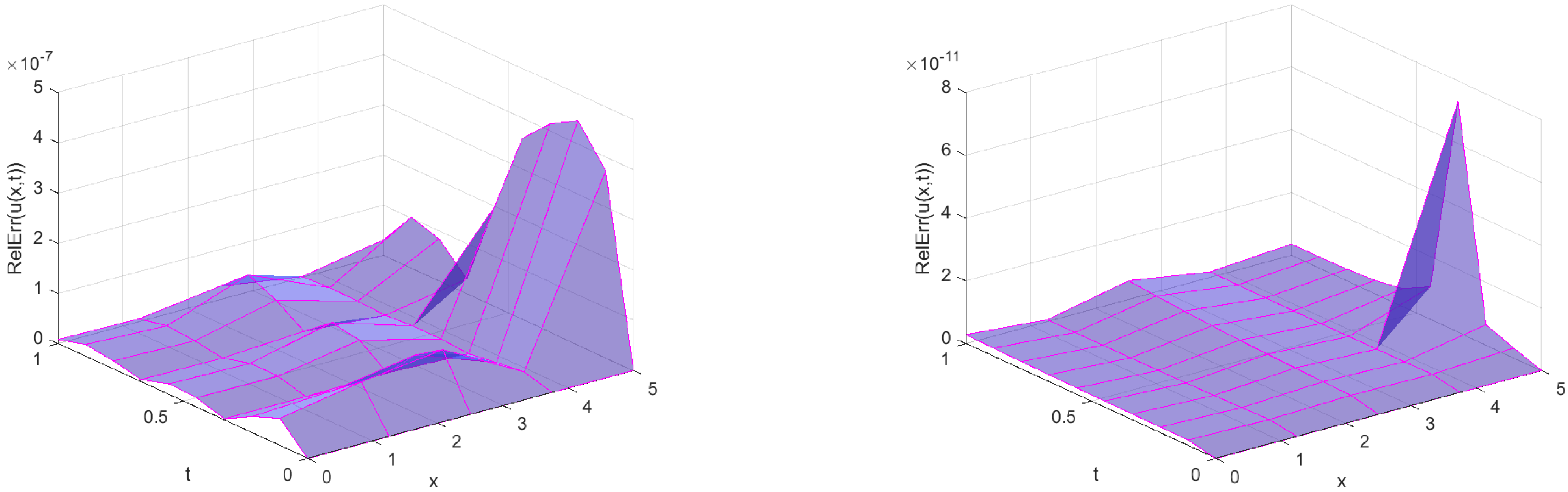
The relative errors for Midpoint rule and Talbot inverse methods are plotted in Figure 1. Because no boundary conditions are posed for the problem, the largest values of the relative errors are situated at the boundary ${\displaystyle x=L}$.

Table 2. Gauss–Laguerre (GL) and Exponentially-fitted Gauss–Laguerre quadrature (EF-GL) methods results, depending on number of nodes of the quadrature for Example 1.

$N_{GL}$	3	5	8	15
GL Error	${\displaystyle 8.2739}$	${\displaystyle 7.4679}$	${\displaystyle 2.5601}$	${\displaystyle 1.4560}$
GL CPU-time, s	${\displaystyle 0.02}$	${\displaystyle 0.02}$	${\displaystyle 0.05}$	${\displaystyle 0.05}$
EF-GL Error	${\displaystyle 9.4937}$	${\displaystyle 7.9303}$	${\displaystyle 7.5438}$	${\displaystyle 3.9366\times {10}^3}$
EF-GL CPU-time, s	${\displaystyle 0.44}$	${\displaystyle 1.84}$	${\displaystyle 15.84}$	${\displaystyle 430.89}$

presents a comparison of GL and EF-GL quadratures in terms of the maximum relative error and the CPU-time varying the number of nodes ${\displaystyle N_{GL}}$. It is important to notice that the CPU-time may vary from simulation to simulation, thus only the order should be taken into account. In the case of GL quadrature, we find out that the computational time is similar with increasing number of nodes, while the CPU-time for EF-GL method is increasing exponentially. The convergence of the GL quadrature is shown, while taking the results shown in Table 1 into account: the error reduces significantly with an increasing number of nodes. The potential improvement of the GL method by the exponential fitting expectedly has higher computational cost, due to the solution of the nonlinear system at each point of the computational domain. However, the accuracy of the EF-Gl quadrature for this example with oscillating integrand has not been improved when comparing with the standard GL rule. Thus, it will not be considered in further more complicated examples.

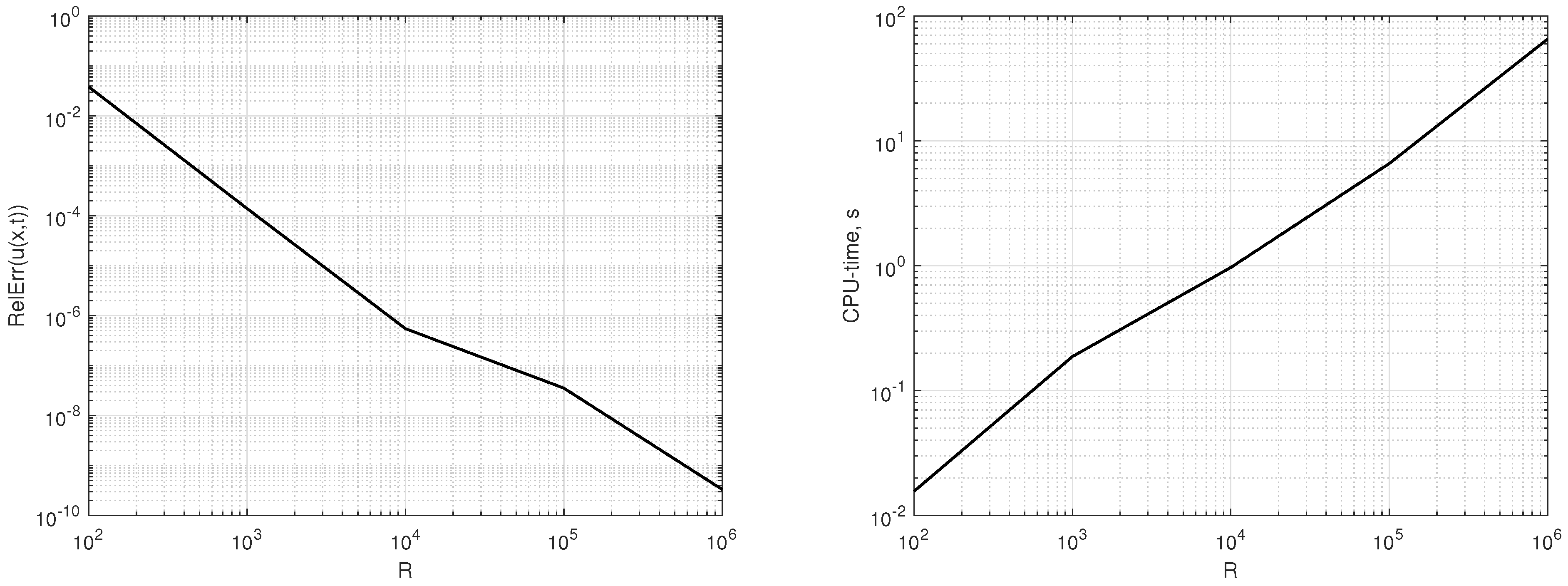
The accuracy of the midpoint rule depends on the truncation ${\displaystyle R}$ and step size ${\displaystyle h_{MP}}$. A bigger domain, as well as smaller step size, lead to an increased computational time. Figure 2 presents the plots of errors and the CPU-time for fixed step size ${\displaystyle h_{MP}={10}^{-1}}$ with respect to increasing domain. The accuracy in dependence on the step size ${\displaystyle h_{MP}}$ is also studied. In

Table 3. The maximum relative error and computational time of the midpoint quadrature rule with respect to step size $h_{MP}$ for Example 1.

$h_{MP}$	Error	CPU-Time, s
${\displaystyle 1/1}$	${\displaystyle 2.8832\times {10}^{-1}}$	${\displaystyle 0.06}$
${\displaystyle 1/2}$	${\displaystyle 3.1862\times {10}^{-2}}$	${\displaystyle 0.06}$
${\displaystyle 1/4}$	${\displaystyle 7.0942\times {10}^{-5}}$	${\displaystyle 0.19}$
${\displaystyle 1/8}$	${\displaystyle 4.4700\times {10}^{-7}}$	${\displaystyle 0.22}$
${\displaystyle 1/16}$	${\displaystyle 4.4699\times {10}^{-7}}$	${\displaystyle 0.53}$
${\displaystyle 1/32}$	${\displaystyle 4.4699\times {10}^{-7}}$	${\displaystyle 1.03}$
${\displaystyle 1/64}$	${\displaystyle 4.4699\times {10}^{-7}}$	${\displaystyle 1.47}$

, the maximum relative error is reported for various ${\displaystyle h_{MP}}$ and fixed ${\displaystyle R={10}^4}$. The maximum relative error is decreasing with step size until ${\displaystyle 4.4699\times {10}^{-7}}$ (${\displaystyle h_{MP}=1/16}$); further fragmentation of the step size does not reduce the error for ${\displaystyle R={10}^4}$.

5.2. Deterministic PDE with Non-Constant Coefficients

In the case of non-constant coefficients in (13), the analytical solution is not always available; thus, FDM is applied to construct a reference numerical solution. Note that the function ${\displaystyle U(x,s)}$ that is used in expression (17) means the value of the numerical solution of the ODE (13) at the fixed point ${\displaystyle x}$ for fixed parameter ${\displaystyle s}$.

Equation (13) is discretized by the central differences on the same mesh ${\displaystyle \left\{x_j\right\}}$, ${\displaystyle j=0,\dots ,N_x}$, as follows

$$\frac{U_{j+1}-2U_j+U_{j-1}}{h^2}+\frac{b\left(x_j\right)}{a\left(x_j\right)}\frac{U_{j+1}-U_{j-1}}{2h}+\frac{c-s^2}{a\left(x_j\right)}{U}_j=-\frac{s{f}_0\left(x_j\right)+f_1\left(x_j\right)}{a\left(x_j\right)},j=1,\dots ,N_x-1,$$

(34)

where ${\displaystyle U_j}$ stands for the approximated value of ${\displaystyle U(x,s)}$ at the node ${\displaystyle x_j}$. The values at the boundaries are found from the boundary conditions by applying the Laplace transform

$$U_0=\mathcal{L}\left[g_0\left(t\right)\right],U_{N_x}=\mathcal{L}\left[g_1\left(t\right)\right].$$

(35)

Hence, the integrand (17) has to be evaluated at each fixed node of the computational grid in order to approximate integral (15), which provokes a significant augment of the CPU-time. In the next example, we increase the complexity by regarding a variable coefficients deterministic problem.

Because the analytical solution for the deterministic PDE problem in general form (7) is not available, a numerical method has to be employed to obtain the reference numerical solution. We consider an explicitly centred in time and space finite difference scheme for the mesh function ${\displaystyle u_j^n\approx u(x_j,t^n)}$:

$$\frac{u_j^{n+1}-2u_j^n+u_j^{n-1}}{{(∆t)}^2}=a\left(x_j\right)\frac{u_{j+1}^n-2u_j^n+u_{j-1}^n}{{(∆x)}^2}+b\left(x_j\right)\frac{u_{j+1}^n-u_{j-1}^n}{2∆x}+c{u}_j^n,$$

(36)

where ${\displaystyle j=1,\dots ,N_x}$, ${\displaystyle n=2,\dots ,N_t}$. The initial conditions (8) are used in order to obtain the solution at the first time levels ${\displaystyle t^0}$ and ${\displaystyle t^1}$. The derivative in (8) is approximated by the forward difference. Because the considered scheme is conditionally stable, the step sizes ${\displaystyle ∆t}$ and ${\displaystyle ∆x}$ are chosen to guarantee the stability. In order to obtain a good approximation, which could be considered as the reference solution, the mesh should be chosen appropriately fine.

Example 2.

Let us consider a deterministic vibrating string problem (7) on rectangle ${\displaystyle [0,L]\times [0,T]}$, ${\displaystyle L=0.5}$, ${\displaystyle T=0.2}$. We set non-constant coefficients ${\displaystyle a\left(x\right)=9x+1}$, ${\displaystyle b=-e^x}$, ${\displaystyle c=-5}$, initial conditions ${\displaystyle f_0\left(x\right)=x(x-L)}$ and ${\displaystyle f_1\left(x\right)=0}$, and boundary conditions ${\displaystyle g_0\left(t\right)=g_1\left(t\right)=0}$.

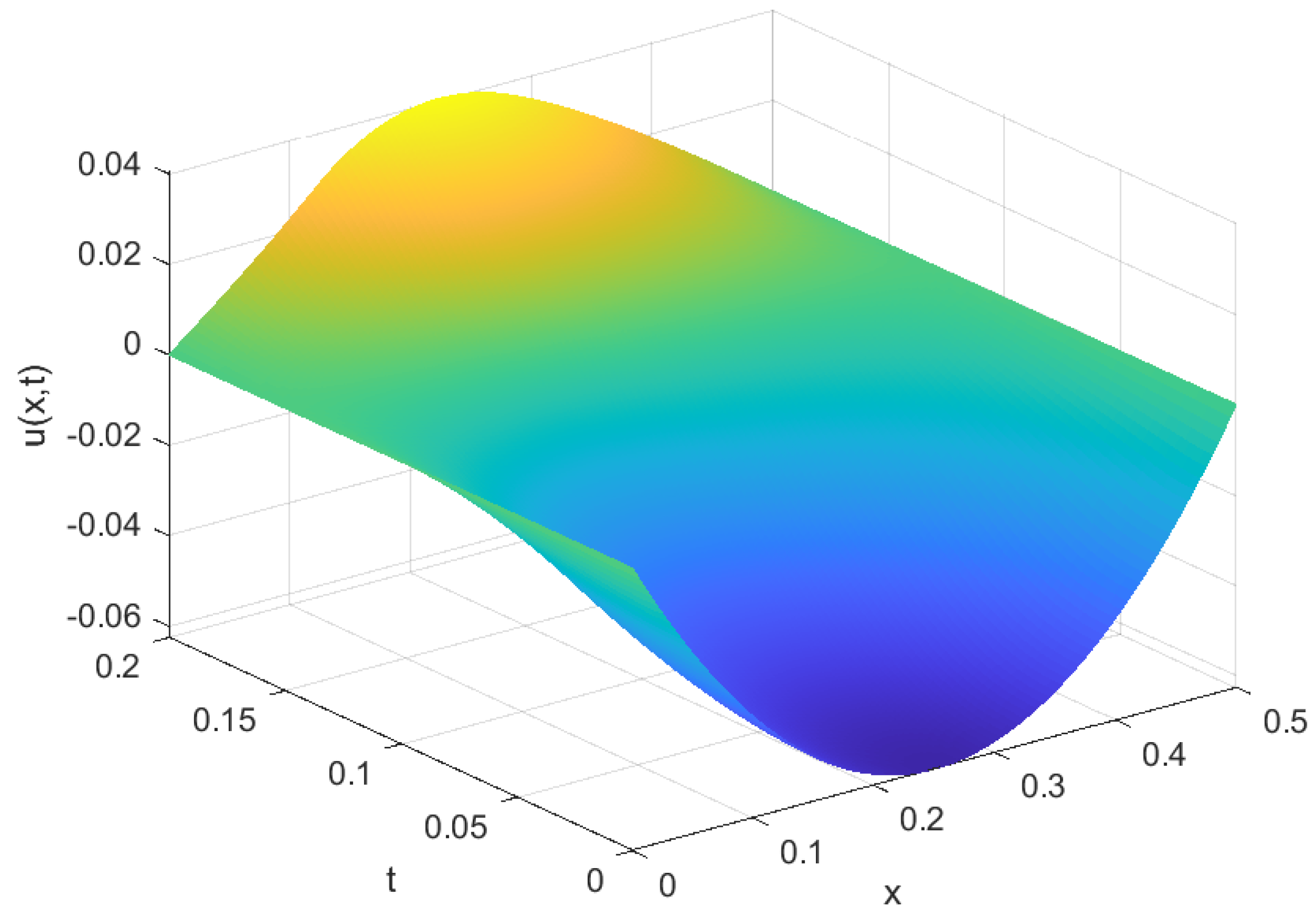
The numerical solution is constructed by the Algorithm 1, choosing ${\displaystyle N_x=10}$, ${\displaystyle N_t=5}$. For the midpoint rule, ${\displaystyle N=100}$ and ${\displaystyle R=100}$ are used.

Table 4. A comparison of various methods of numerical integration for Example 2.

Method	Error	CPU-Time, s
Midpoint quadrature	${\displaystyle 4.5628\times {10}^{-2}}$	${\displaystyle 116.38}$
Talbot inverse	${\displaystyle 7.1305\times {10}^{-2}}$	${\displaystyle 51.00}$
Gauss-Laguerre (9 nodes)	${\displaystyle 7.4450\times {10}^{-1}}$	${\displaystyle 5.00}$
Gauss-Laguerre (25 nodes)	${\displaystyle 7.9014\times {10}^{-2}}$	${\displaystyle 17.48}$

presents the comparison of the methods in terms of maximum relative error and computational time. The reference solution is the numerical solution that is computed by the FDM (36) in refined mesh (${\displaystyle N_x=100}$, ${\displaystyle N_t}$ = 16,000), which preserves the stability of the scheme. Because an explicit method is used and no iterative procedures are needed for solving nonlinear system at each time-level, the total computational time is comparably small: 0.15 s. Figure 3 plots the reference solution.

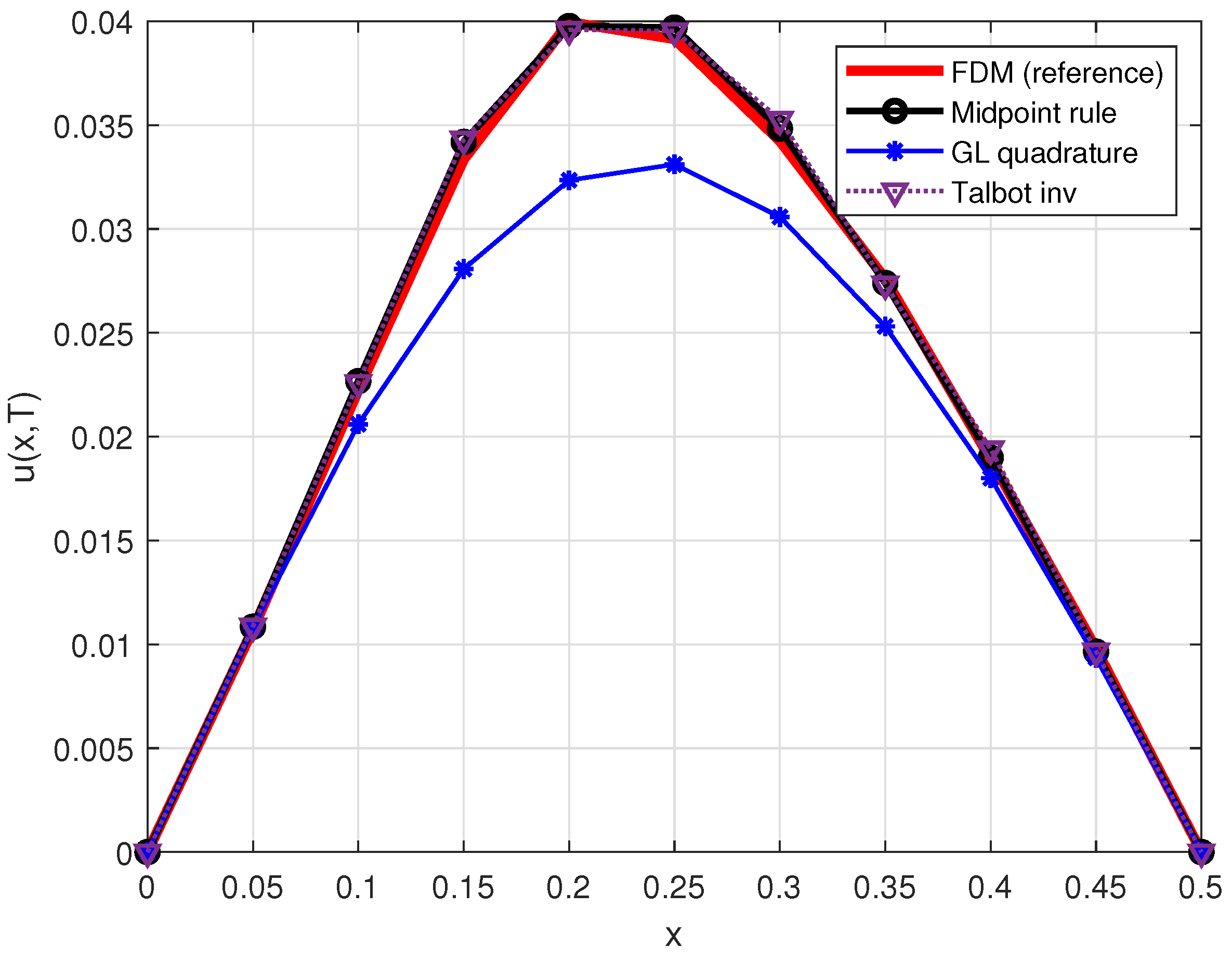
Figure 4 plots the solution at the moment ${\displaystyle t=T}$. The midpoint rule and Talbot inverse method perform more accurately than GL quadrature of nine nodes, but they require more computational time due to larger number of calls of integrand (17). However, taking 25 nodes in the GL quadrature, the accuracy has been improved significantly.

5.3. Random PDE with Constant Coefficients

In this subsection, we deal with random models with constant coefficient random variables. It is remarkable that, in this case, we need not only the computation of the approximation s.p. solution, but also the computation of its statistical moments.

Example 3.

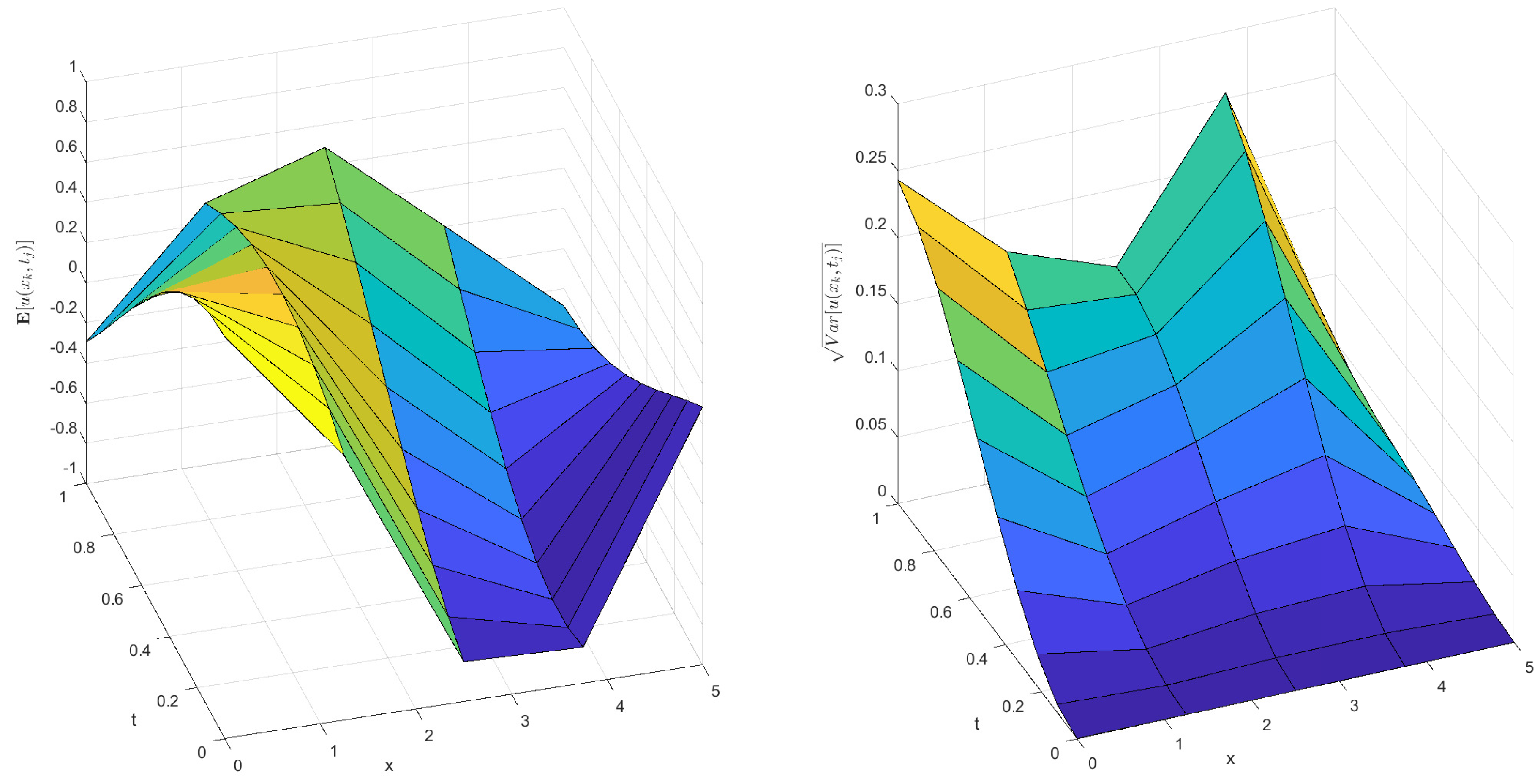
We consider a random version of problem (25), with ${\displaystyle a\sim \mathcal{N}(2,0.25)}$, ${\displaystyle b,c\sim Beta(2,5)}$. In order to approximate the mean and variance of the solutions, the Monte Carlo method with ${\displaystyle N_{MC}}$ simulations is used.

Expectation and variance of the exact solution for the random hyperbolic PDE (25) are plotted in Figure 5. As in previous examples, we compare the proposed methods of integration and Laplace inverse in terms of maximum relative error and computational time.

Table 5. Comparison of various methods of numerical integration for the random hyperbolic PDE (25) with ${\displaystyle a\sim \mathcal{N}(2,0.25)}$, ${\displaystyle b,c\sim \mathrm{Beta}(2,5)}$.

Method	Error of Mean	Error of Variance	CPU-Time, s
${\displaystyle N_{MC}=500}$
Midpoint rule	${\displaystyle 5.6048\times {10}^{-2}}$	${\displaystyle 2.3034\times {10}^{-2}}$	${\displaystyle 4.88}$
Talbot inverse	${\displaystyle 5.0744\times {10}^{-2}}$	${\displaystyle 2.3032\times {10}^{-2}}$	${\displaystyle 6.83}$
GL quadrature (3 nodes)	${\displaystyle 1.9009\times {10}^{-1}}$	${\displaystyle 2.1436\times {10}^{-1}}$	${\displaystyle 2.92}$
${\displaystyle N_{MC}=1000}$
Midpoint rule	${\displaystyle 4.1520\times {10}^{-2}}$	${\displaystyle 2.5102\times {10}^{-2}}$	${\displaystyle 7.52}$
Talbot inverse	${\displaystyle 4.0345\times {10}^{-2}}$	${\displaystyle 2.5102\times {10}^{-2}}$	${\displaystyle 12.67}$
GL quadrature	${\displaystyle 1.9086\times {10}^{-1}}$	${\displaystyle 2.1503\times {10}^{-1}}$	${\displaystyle 5.64}$
${\displaystyle N_{MC}=2000}$
Midpoint rule	${\displaystyle 3.7210\times {10}^{-2}}$	${\displaystyle 1.2823\times {10}^{-2}}$	${\displaystyle 16.88}$
Talbot inverse	${\displaystyle 3.1905\times {10}^{-2}}$	${\displaystyle 1.2823\times {10}^{-2}}$	${\displaystyle 24.86}$
GL quadrature	${\displaystyle 1.9001\times {10}^{-1}}$	${\displaystyle 2.1443\times {10}^{-1}}$	${\displaystyle 11.30}$
${\displaystyle N_{MC}=4000}$
Midpoint rule	${\displaystyle 4.6382\times {10}^{-2}}$	${\displaystyle 9.8022\times {10}^{-3}}$	${\displaystyle 32.89}$
Talbot inverse	${\displaystyle 4.1078\times {10}^{-2}}$	${\displaystyle 9.7971\times {10}^{-3}}$	${\displaystyle 51.09}$
GL quadrature	${\displaystyle 1.8993\times {10}^{-1}}$	${\displaystyle 2.1581\times {10}^{-1}}$	${\displaystyle 24.31}$

presents the results for various ${\displaystyle N_{MC}}$. The CPU-time refers to the total computational time for all ${\displaystyle N_{MC}}$ simulations. Note that, for 1000 simulations, the exact solution (26)–(27) requires ${\displaystyle 28.41}$ s to perform the simulations. Thus, Midpoint rule (${\displaystyle R=100}$, ${\displaystyle h=0.1}$), Talbot inverse and GL quadrature require less computational time than calculation by the exact formula. As expected, the computational time is increasing with the number of simulations linearly, but errors preserve the order in most cases.

5.4. Random PDE with Non-Constant Coefficients

To complete the study, a random variable coefficient problem is considered.

Example 4.

The vibration of the string in ${\displaystyle [0,L]}$ is described by Equation (7), subject to the initial conditions ${\displaystyle f_0\left(x\right)=x(x-L)}$ and ${\displaystyle f_1\left(x\right)=0}$; and boundary conditions ${\displaystyle g_0\left(t\right)=g_1\left(t\right)=0}$. We set up the parameters:

$$L=0.5,T=0.2,a\left(x\right)=\phi x+1,\phi \sim \mathcal{N}(9,0.5),b\left(x\right)=-e^x,c\sim Beta(2,5).$$

(37)

Unlike the deterministic Example 2 with non-constant coefficients where FDM provides a reference analytical solution, reference values are not available here due to the computational complexity that arises in the evaluation of the statistical moments of the approximate stochastic process when time step advances [18]. A survival reference FDM solution is taking the Monte Carlo method for an appropriate set of realizations. In this case, the number of realizations is ${\displaystyle N_{MC}={10}^3}$ and CPU-time is 16,212 s.

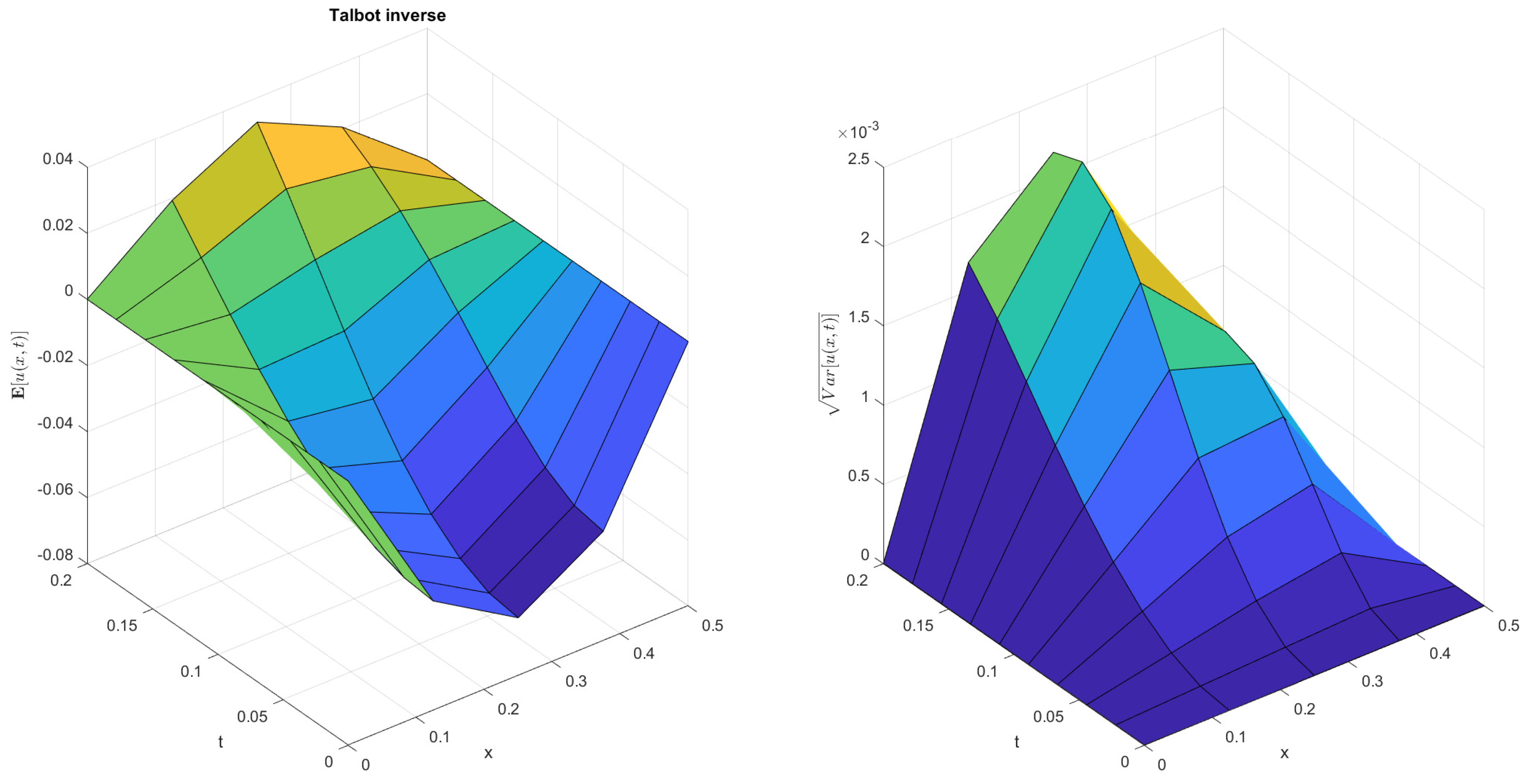
Figure 6 plots the numerical solution. The zero-variance at the boundaries is caused by the boundary conditions. Similar plots are obtained for the considered methods. Thus, we compare them in terms of the maximum relative error, see

Table 6. Comparison of various methods of numerical integration for Example 4, ${\displaystyle N_{MC}=1000}$.

Method	Error of Mean	Error of Variance	CPU-Time, s
Midpoint rule	${\displaystyle 3.8216\times {10}^{-2}}$	${\displaystyle 2.2638\times {10}^{-2}}$	${\displaystyle \mathrm{65,385.00}}$
Talbot inverse	${\displaystyle 3.4976\times {10}^{-2}}$	${\displaystyle 2.1375\times {10}^{-2}}$	${\displaystyle \mathrm{28,965.54}}$
GL quadrature (9 nodes)	${\displaystyle 1.8671\times {10}^{-1}}$	${\displaystyle 2.5603\times {10}^{-2}}$	${\displaystyle 7192.14}$

. As it is expected from the previous examples, the most accurate solution is obtained by the midpoint rule and Talbot inverse, although this advantage pays the price of additional computational cost.

6. Conclusions

The solution of a random hyperbolic PDE problem is a challenging task that is demanded in many practical applications. Computing an expression of the approximating stochastic process makes the computation of its statistical moments available. In this paper, we propose a combination of the random Laplace transform with the numerical integration techniques for its inverse, and the Monte Carlo method for the evaluation of numerical solution of the transformed problem at a particular required point.

The Monte Carlo simulations require a fast and efficient basis numerical algorithm for solving deterministic hyperbolic PDE problem, for every fixed realization. FDM could not be an option due to the high computational cost and memory requirements. In order to avoid the numerical differentiation of the PDE, Laplace transform is applied, which results in ODE equation. In some cases, as it has been shown in present paper, the analytical solution of ODE is known; thus, we use numerical integration methods for inverse Laplace transform. If the solution of ODE is not available, then numerical techniques for boundary value problem have to be employed.

Several numerical integration methods have been considered: midpoint rule and GL-quadrature for improper integrals. However, due to the oscillatory behaviour of the integrand function GL quadrature with a small number of nodes shows comparatively poor results, while the midpoint rule is comparable with Talbot’s Laplace inverse for random hyperbolic PDEs. The proposed complex analytic-numerical approach is compared with the classical explicit FDM scheme for the original random PDE problem.

References

- Pettersson, M.P.; Iaccarino, G.; Nordström, J. Polynomial Chaos Methods for Hyperbolic Partial Differential Equations. Numerical Techniques for Fluid Dynamics Problems in the Presence of Uncertainties; Springer International Publishing: Cham, Switzerland, 2015; p. 214. [Google Scholar]
- Yeh, K.C.; Liu, C.H. Wave Propagation in Random Media. In Theory of Ionospheric Waves; Academic Press: Cambridge, MA, USA, 1972; Volume 17, pp. 308–366. [Google Scholar] [CrossRef] [Green Version]
- Gibson, W.C. The Method of Moments in Electromagnetics; Taylor & Francis Group: Abingdon, UK, 2008. [Google Scholar]
- Vergara, R.C. Development of Geostatistical Models Using Stochastic Partial Differential Equations. Ph.D. Thesis, Université Paris Sciences et Lettres, Paris, France, 2018. [Google Scholar]
- Soong, T. Random Differential Equations in Science and Engineering, 1st ed.; Academic Press: Cambridge, MA, USA, 1973; Volume 103. [Google Scholar]
- Kroese, D.P.; Taimre, T.; Botev, Z. Handbook of Monte Carlo Methods; John Wiley & Sons: New York, NY, USA, 2011. [Google Scholar]
- Asmussen, S.; Glynn, P. Stochastic Simulation: Algorithms and Analysis; Springer Science & Business Media: Berlin/Heidelberg, Germany, 2007; Volume 57. [Google Scholar]
- Casabán, M.C.; Company, R.; Jódar, L. Non-gaussian quadrature integral transform solution of parabolic models with a finite degree of randomness. Mathematics 2020, 8, 1112. [Google Scholar] [CrossRef]
- Davies, B.; Martin, B. Numerical inversion of the laplace transform: A survey and comparison of methods. J. Comput. Phys. 1979, 33, 1–32. [Google Scholar] [CrossRef]
- Stehfest, H. Algorithm 368: Numerical Inversion of Laplace Transforms [D5]. Commun. ACM 1970, 13, 47–49. [Google Scholar] [CrossRef]
- Talbot, A. The Accurate Numerical Inversion of Laplace Transforms. IMA J. Appl. Math. 1979, 23, 97–120. [Google Scholar] [CrossRef]
- Defreitas, C.L.; Kane, S.J. The noise handling properties of the Talbot algorithm for numerically inverting the Laplace transform. J. Algorithms Comput. Technol. 2018, 13, 1748301818797069. [Google Scholar] [CrossRef] [Green Version]
- Iserles, A. On the numerical quadrature of highly-oscillating integrals I: Fourier transforms. IMA J. Numer. Anal. 2004, 24, 365–391. [Google Scholar] [CrossRef]
- Davis, P.J. Methods of Numerical Integration; Dover Publications: Mineola, NY, USA, 2007; p. 612. [Google Scholar]
- Casabán, M.C.; Company, R.; Egorova, V.N.; Jódar, L. Integral transform solution of random coupled parabolic partial differential models. Math. Methods Appl. Sci. 2020, 43, 8223–8236. [Google Scholar] [CrossRef]
- Casabán, M.C.; Cortés, J.C.; Jódar, L. A random Laplace transform method for solving random mixed parabolic differential problems. Appl. Math. Comput. 2015, 259, 654–667. [Google Scholar] [CrossRef]
- Arnold, L. Stochastic Differential Equations Theory and Applications; John Wiley: Hoboken, NJ, USA, 1974. [Google Scholar]
- Casabán, M.C.; Company, R.; Jódar, L. Numerical Integral Transform Methods for Random Hyperbolic Models with a Finite Degree of Randomness. Mathematics 2019, 7, 853. [Google Scholar] [CrossRef] [Green Version]
- Iserles, A.; Nørsett, S.P. On Quadrature Methods for Highly Oscillatory Integrals and Their Implementation. BIT Numer. Math. 2004, 44, 755–772. [Google Scholar] [CrossRef] [Green Version]
- Shao, T.S.; Frank, T.C.; Chen, R.M. Tables of zeros and Gaussian weights of certain associated Laguerre polynomials and the related generalized Hermite polynomials. Math. Comput. 1964, 18, 598–616. [Google Scholar] [CrossRef]
- Conte, D.; Ixaru, L.G.; Paternoster, B.; Santomauro, G. Exponentially-fitted Gauss-Laguerre quadrature rule for integrals over an unbounded interval. J. Comput. Appl. Math. 2014, 255, 725–736. [Google Scholar] [CrossRef]
- Abate, J.; Whitt, W. A Unified Framework for Numerically Inverting Laplace Transforms. INFORMS J. Comput. 2006, 18, 408–421. [Google Scholar] [CrossRef]
- Polyanin, A.D.; Nazaikinskii, V.E. Handbook of Linear Partial Differential Equations for Engineers and Scientists, 2nd ed.; CRC Press: Boca Raton, FL, USA, 2016; p. 1643. [Google Scholar]
- Shampine, L. Vectorized adaptive quadrature in MATLAB. J. Comput. Appl. Math. 2008, 211, 131–140. [Google Scholar] [CrossRef] [Green Version]
Figure 1.
Distribution of the relative error among space and time for midpoint rule (left) and Talbot inverse (right) methods in Example 1.
Figure 2.
Error and total computational time of the midpoint rule with respect to the domain size with fixed for Example 1.
Figure 3.
Reference solution for Example 2 computed by the finite difference method (FDM) (36).
Figure 4.
Numerical solution for Example 2 at the moment obtained by considered methods.