Empirical Assessment of Machine Learning Techniques for Software Requirements Risk Prediction

Abstract

Software risk prediction is the most sensitive and crucial activity of Software Development Life Cycle (SDLC). It may lead to the success or failure of a project. The risk should be predicted earlier to make a software project successful. A model is proposed for the prediction of software requirement risks using requirement risk dataset and machine learning techniques. In addition, a comparison is made between multiple classifiers that are K-Nearest Neighbour (KNN), Average One Dependency Estimator (A1DE), Naïve Bayes (NB), Composite Hypercube on Iterated Random Projection (CHIRP), Decision Table (DT), Decision Table/Naïve Bayes Hybrid Classifier (DTNB), Credal Decision Trees (CDT), Cost-Sensitive Decision Forest (CS-Forest), J48 Decision Tree (J48), and Random Forest (RF) achieve the best suited technique for the model according to the nature of dataset. These techniques are evaluated using various evaluation metrics including CCI (correctly Classified Instances), Mean Absolute Error (MAE), Root Mean Square Error (RMSE), Relative Absolute Error (RAE), Root Relative Squared Error (RRSE), precision, recall, F-measure, Matthew’s Correlation Coefficient (MCC), Receiver Operating Characteristic Area (ROC area), Precision-Recall Curves area (PRC area), and accuracy. The inclusive outcome of this study shows that in terms of reducing error rates, CDT outperforms other techniques achieving 0.013 for MAE, 0.089 for RMSE, 4.498% for RAE, and 23.741% for RRSE. However, in terms of increasing accuracy, DT, DTNB, and CDT achieve better results.

1. Introduction

The development of software consistently faces uncertain occasions that may have negative impact on the success of software development, such occasions are called software risks [1]. The risks have a vital impact on software requirements. They turn out to be the reason for damage to the software or stakeholders [1,2,3]. The Standish Group research illustrates an astounding 31.1% of projects terminate before completion while merely 16.2% software projects are completed on-time and with-in-the-budget. In bigger organizations, the result is even worse: only 9% of the projects are deployed on-time and within the budget. Moreover, in the completed projects, many are no more than a mere shadow of their original specification requirements. Projects completed by the largest American companies have only approximately 42% of the originally proposed functionalities [4]. Risk assessment has basically two strategies, proactive and reactive. According to the literature the reactive strategy is not a mature strategy to assess the risk, since it increases the budget schedule and resources but degrades the quality and success of the project. Therefore, a proactive strategy has been employed using machine learning techniques to reduce the chances of project failure [5]. Also, the prediction of risks at this stage is more beneficial and raises the productivity of software. It also helps in reducing the probabilities of software project failure when risks are managed properly in requirements gathering phase [1].

In our preliminary paper [1], a risk dataset was proposed that is comprised of software requirements, risks attributes and relations between them, which are also necessary for the prediction of risks in the new software projects. The dataset can be used to predict risks over the Software Requirements Specification (SRS) of a project using machine learning techniques.

In this study, the main focus is on the empirical analysis of ten Machine Learning (ML) techniques. These include: K-nearest Neighbors (KNN), Average One Dependency Estimator (A1DE), Naïve Bayes (NB), Composite Hypercube on Iterated Random Projection (CHIRP), Decision Tree (DT), Decision Table/Naïve Bayes Hybrid Classifier (DTNB), Credal Decision Tree (CDT), CS-Forest, J48, and Random Forest (RF). All these techniques are explored first time for risk prediction and are employed on our previously proposed dataset [6].

It is relevant to note that although 10 different ML techniques are chosen on the basis of a pre-selection process where a comparison has been made among these classifiers on the basis of their effective results such as fast training/build time and accuracy on the different datasets as shown in

Table 1. Selection of for ML Classifiers.

Classifier	Dataset	Training Time	Input Scale	Input Data Types	Accuracy
	-	Time to build model	Low: Instances < 1000 Medium: > 1000 Instances < 10,000 High: Instances > 10,000	Numeric, String, Nominal	-
KNN	Medical Imaging Datasets [7]	Time < 1 min	Large	-	Mean ± standard deviation (0.6 to 0.9)
A1DE	UCI Datasets [8]	Time < 1 min	Medium to Large	Numeric, Nominal	CCI (56% to 69%)
NB	UCI Datasets [8]	Time < 1 min	Medium to Large	Numeric, Nominal	CCI (55%)
CHIRP	UCI datasets [9]	-	Medium to Large	Numeric, Nominal	Mean standard test error (−1 to 0)
DT	Online Shopping Dataset [10]	Time < 1 min	Medium	Numeric, Nominal	CCI (76.28 %)
DTNB	UCI datasets [11]	-	Low to medium	Numeric, Nominal	Mean AUC and standard deviation (0.6 to 1.0)
CDT	UCI Datasets [8]	Time < 1 min	Medium to Large	Numeric, Nominal	CCI (63 %)
CS-Forest	Brazilian Bank Dataset [12]	-	Medium	Numeric, Nominal	Accuracy (95%)
J48	Liver Disorder Dataset (UCI) [13]	Time < 1 min	low	Numeric, Nominal	Accuracy (97.75%)
RF	Medical University Hospital [14]	-	Low	Numeric, Nominal	Accuracy (95%)
MPL (NN)	Medial Diagnosis Classification Datasets [15]	-	Low to Medium	Numeric, Nominal	Accuracy (No of correct predictions/total predictions) 0.9

.

Moreover, these classifiers are tested and observed on the basis of their CCI on Risk dataset [1], using 10 cross fold validation test for the selection of further studies. It is necessary to mention that the Neural Network-based classifiers were not considered in this paper. NN-based techniques have some disadvantages, e.g., they usually require a large size of input, produce unexpected behavior due to the black boxes, learning process may take long time with no guarantee of success, it is difficult to determine the proper network structure and it initially depends on format mechanism of the input [16,17]. The NN typically need thousands or millions of labeled samples [17,18], whereas the risk dataset contains only 299 instances to train a NN. In fact, in our preliminary selection process the CCI obtained were not good enough to keep it further in this study, therefore we kept NN out of this study. The Pre-selection comparison is presented in

Table 2. Pre-selection comparison of classifiers.

Classifier	CCI%
KNN	58.2
A1DE	91.0
NB	91.0
CHIRP	44.0
DT	98.0
DTNB	98.0
CDT	98.0
CS-Forest	73.2
J48	96.3
RF	83.2
NN (Multi-Layer perceptron)	39.1

.

The detail experiments are conducted in this study to show which ML technique outperforms for risk prediction in the earliest phase of SDLC.

The foremost contributions of this research are as follow:

• We selected ten different ML techniques (KNN, A1DE, NB, CHIRP, DT, DTNB, CDT, CS-Forest, J48, and RF) for Model Evaluation and Comparison.
• We demeanour a series of try-outs on our published dataset [6].
• To reveal insight to the experimental outcomes, evaluation is accomplished using CCI, MAE, RMSE, RAE, RRSE, precision, recall, F-measure, MCC, ROC Area, PRC Area and Accuracy.

2. Overview of Risk Prediction

This research aims to resolve the predicament of late identification of risk and their effect on quality, schedule, and budget of the ongoing software project. Because most recent risk prediction methodologies have potential to measure software risks in the upcoming stages, naturally from software design phase or code of the software life cycle, these methodologies have potential to identify risks but have limited ability in avoiding these risks from occurring [1]. The risks are caused by several factors during the SDLC, and can lead to failure of the software project [2,3,4]. These factors are considered to be one of the main reasons of software failure causes, they result from the less software engineering theory principles and techniques. These factors should be resolved as soon as possible to lessen the unexpected failure of the software project.

As per our previous paper, we concluded that no dataset found that contain essential attributes for software requirement risks. Therefore, in that paper we introduced a dataset containing attributes and their relations between software requirements and risks [1]. Moreover, a model is needed to predict risk using the risk dataset using classification techniques of machine learning.

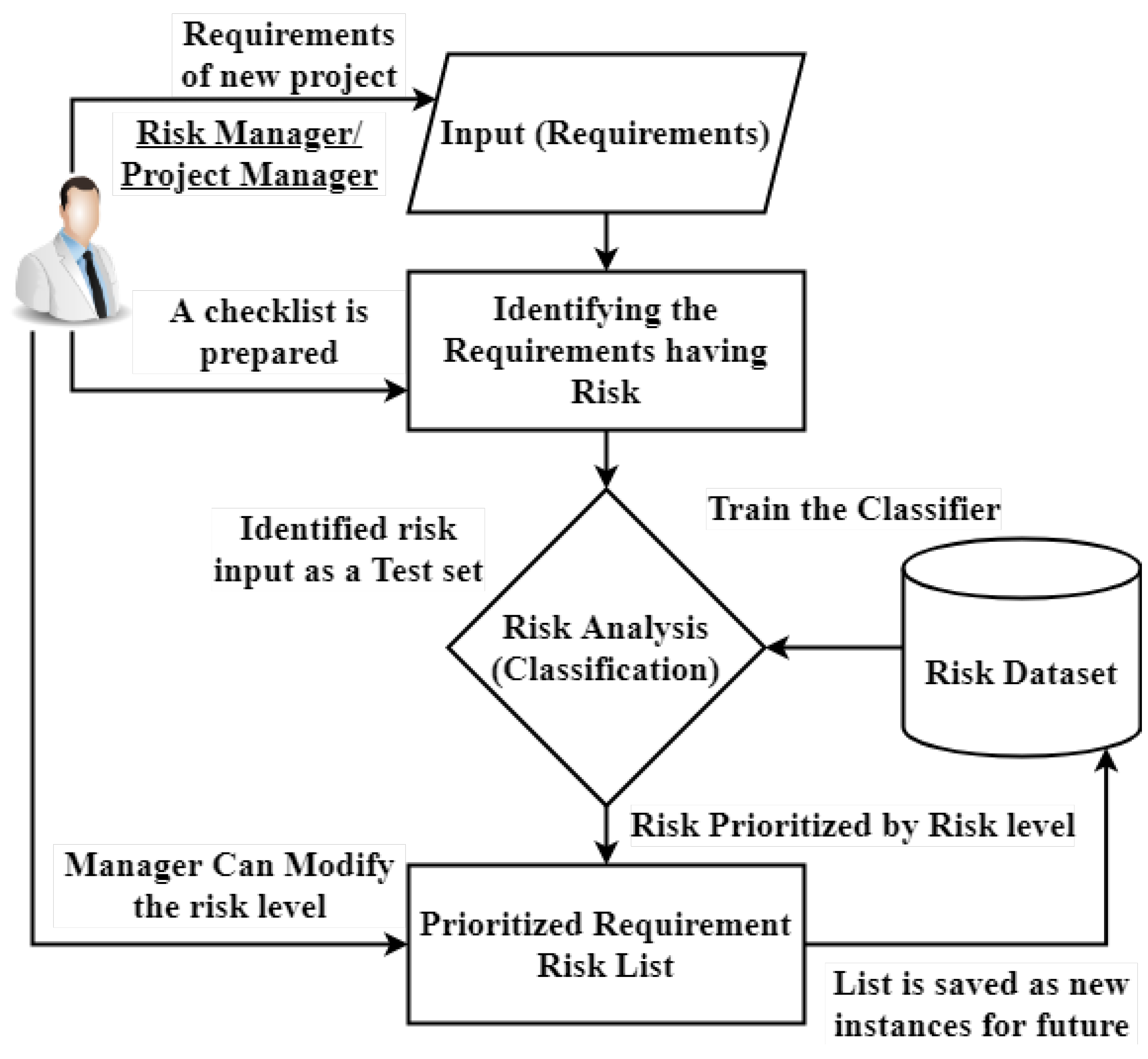
The core aspects of the software project which need to be improved are quality of overall project, budget, and schedule by predicting the risk earlier. The risk prediction model helps to identify risk level of an instance (software requirement) of new project using risk dataset. However, the project/risk manager will be able to customize and manage the overall process of risk prediction. The basic model of the risk prediction using ML techniques has been introduced. This model contains four main components as demonstrated in Figure 1 and briefly discussed below.

• Risk Identification: The very first stage of Software Risk Prediction Model is Risk Identification, where the Risk Manager/Project manager will identify the hazards that may distract the time, resources, or costs of the project. A hazard is an unfortunate event if it occurs, and is detrimental to the successful completion of the project. It is performed using “checklist”. The requirements from SRS with risk threats are marked checked for further analysis. The checklist is then headed to the next stage [5].
• Risk Analysis: The identified risks then convert into decision-making information. The probability and the significance of each risk is assessed through risk analysis, the risks are transform into decision-making information that were identified [5]. Each risk is then measured and a decision made about the possibility and the seriousness of the risk. The attribute “Risk Level” in the risk dataset helps to classify the requirements among five risk levels [1].
• Risk Prioritization: This is the output stage of the Model, where the analyzed Risks are Prioritized. The requirements having high “risks level” are transferred above in the list and the requirements having low “risks level” drop to the bottom.
• Requirement risk Dataset: The Dataset contains Risk measures for software requirements are available on Zenodo datasets [6]. The risk dataset comprises of the attributes that are related to risks and requirements of software project [1].

In the proposed model, the requirement set is input to the model to produce the risk level of the requirements, by which the project manager/domain expert can easily plan and mitigate the risks at earlier stages.

3. The Research Framework

The risk dataset is comprised of the attributes that are related to risks and requirements of software project [1]. These risks have a negative impact on the success of the software development. In the proposed model, the requirement set is input to the model to produce the risk level of the requirements, by which the project manager/domain expert can easily plan and mitigate the risks at earlier stages.

The research has two main phases, i.e., risk prediction model for software requirements and Model Evaluation and Comparison. The risk-oriented dataset and its filtration was necessary for our proposed model since that is done in our preliminary work [1], The dataset is openly available for further exploration and improvement. The proposed research framework is demonstrated in Figure 2.

The first step of the research is Preparation of the Model for requirement risk prediction; here we have chosen the classifiers on the basis of Table 1. The second step is Model Evaluation and Comparison, here in this step we evaluated model on chosen classifiers using Risk dataset for comparison to choose best suitable classifier. In the third step the Proposed model is validated using new set of requirements. The last step contains the results of Model Validation.

4. Model Evaluation and Comparison

In this phase, KNN, A1DE, NB, CHIRP, DT, DTNB, CDT, CS-Forest, J48, and RF are employed on the risk dataset. We trained these models on WEKA (Waikato Environment for Knowledge Analysis) Tool and the parameters of every algorithm were tuned to take best output into consideration and validated these using 10-cross fold with the discrete dataset [1], and supplied a sample set of 299 instances to the model. The 10-fold cross-validation test is applied to every classifier to assess its performance. The provided learning set is break up into 10 distinct subsets of a similar size. The “fold” here is referred to as the number of subsets created. These subsets then are used as one for training and others for testing and this loop is performed until every subset is being trained and tested by the model [19]. We applied minimum and maximum number of k folds to the dataset, but they mostly decrease the efficiency due to change in the percentage of training and testing. Whereas the 10-fold cross validation performed better as compared to any other selection of k folds. Therefore, the 10-fold cross validation method is selected to validate the models and to avoid over fitting and under fitting during the training process [19]. The evaluation is done on the basis of CCI, MAE [20,21], RMSE [20,21,22], RAE [23], RRSE [23], precision [21,24], recall [21], F-measure [21], MCC [25,26], ROC Area [27], PRC Area [28] and Accuracy [27,29,30]. The results are presented in Section 5.

4.1. Requirement Risk Dataset

The dataset is taken from [1] which is collected through different SRS of different open source projects that include,

• Transaction processing system: This SRS has 118 requirements collectively.
• Management information system: That contains the E-Store product features. This SRS collectively contains 87 Requirements.
• Enterprise system: This SRS identifies requirements focused on medical records and the associated diagnostics. This SRS has 59 requirements.
• Safety critical system: The intelligent Traffic Expert Solution for road traffic control System offers the ability to acquire real-time traffic information. It has 35 requirements.

The dataset contains 299 instances (Requirements) collectively as mentioned in

Table 3. Projects and number of instances.

Project	Instances
Transaction Processing System	118
Management Information System	87
Enterprise System	59
Safety Critical System	35
Total	299

.

The data types of the attributes were assigned according to nature and value set of the data which were achieved from Boehm’s risks management [1,31,32] as shown in

Table 4. Risk dataset template.

Attributes	Data Types
Requirements	String
Project Category	Nominal
Requirement Category	Nominal
Risk Target Category	Nominal
Probability	Numeric
Magnitude of Risk	Nominal
Impact	Nominal
Dimension of Risk	Numeric
Affecting No Modules	Numeric
Fixing Duration	Numeric
Fix Cost	Numeric
Priority	Numeric
Risk Level	Nominal

.

4.2. K-Nearest Neighbour

KNN classifiers are instance-based learning techniques where the training feature vectors forecast the class of an unidentified trial data. Classification of trial data is grounded on main stream division of its neighbours (training models). Therefore, trial data is allocated to the class label of training models that ambiances it in majority [3,7,33].

Table 5. CCI and Error Rates details achieved via KNN.

KNN
CCI	174 (58.194%)
MAE	0.170
RMSE	0.405
RAE%	60.638
RRSE%	108.363

and

Table 6. KNN accuracy details.

Class	Precision	Recall	F-Measure	MCC	ROC Area	PRC Area
1	0.480	0.429	0.453	0.401	0.718	0.293
2	0.701	0.711	0.706	0.461	0.743	0.651
3	0.494	0.547	0.519	0.348	0.688	0.392
4	0.537	0.489	0.512	0.430	0.709	0.341
5	0.231	0.188	0.207	0.168	0.586	0.088
Weighted Average	0.578	0.582	0.579	0.406	0.713	0.476

, respectively, present the error rate and accuracy outcomes achieved by KNN using several numbers of k and presented best outcome of results among them. In Table 6, the first rows present the accuracy measures while rows 2–5 present the individual outcomes of each assessment measure. The percentage of CCI is considered to be the outcome of accuracy.

We have applied 10-fold cross validation on the Risk Dataset using KNN, and CCI achieved 174 (58.194%), The MAE is 0.170, RMSE is 0.405, RAE is 60.638 and RRSE is 108.363.

4.3. Average One Dependency Estimator

A1DE is a probabilistic technique, recycled for habitual classification complications. It shows enormously accurate classification by being an average of all-encompassing of a slight space of different Naive Bayes (NB)-like models that have punier independence possibilities than NB. A1DE was essentially planned to address the attribute-independence problems of a standard NB technique. It was intended to address the attribute-independence issues of the predominant NB classifier [34].

Table 7. CCI and Error Rates details achieved via AIDE.

AIDE
CCI	271 (90.635%)
MAE	0.048
RMSE	0.169
RAE%	17.045
RRSE%	45.181

presents the error rate details with CCI, while

Table 8. AIDE accuracy details.

Class	Precision	Recall	F-Measure	MCC	ROC Area	PRC Area
1	0.929	0.929	0.929	0.921	0.998	0.985
2	0.954	0.926	0.940	0.892	0.989	0.989
3	0.880	0.880	0.880	0.840	0.978	0.946
4	0.886	0.867	0.876	0.855	0.959	0.875
5	0.714	0.938	0.811	0.807	0.994	0.822
Weighted Average	0.910	0.906	0.907	0.872	0.983	0.952

presents the overall accuracy outcomes achieved via A1DE.

We have applied 10-fold cross validation on the dataset usin AIDE, the CCI achieved 271 (90.635%) and The MAE is 0.048, RMSE is 0.169, RAE is 17.045 and RRSE is 45.181.

4.4. Naïve Bayes

The NB classifier is a probabilistic statistical classifier. The term “naive” indicates a restrictive independence among attributes or features. The naive supposition decreases computation convolution to a simple multiplication of likelihoods. One main advantage of the NB classifier is its speed of use. That is because it is the greenest technique amid classification techniques. As an effect of this openness, it can punctually contract with an informational index with abundant abilities [35,36]. The CCI and error rate achieved by NB are presented in

Table 9. CCI and Error Rates details achieved via NB.

NB
CCI	272 (90.970%)
MAE	0.042
RMSE	0.160
RAE%	14.993
RRSE%	42.876

as well, while all the accuracy outcomes are listed in

Table 10. NB accuracy details.

Class	Precision	Recall	F-Measure	MCC	ROC Area	PRC Area
1	0.813	0.929	0.867	0.854	0.995	0.948
2	0.976	0.896	0.934	0.887	0.984	0.987
3	0.877	0.947	0.910	0.880	0.985	0.906
4	0.889	0.889	0.889	0.869	0.973	0.952
5	0.824	0.875	0.848	0.840	0.944	0.783
Weighted Average	0.914	0.910	0.911	0.877	0.982	0.947

.

We applied 10-fold cross validation on the dataset using Naive Bayes, and CCI achieved 272 (90.970%). The MAE is 0.042, RMSE is 0.160, RAE is 14.993 and RRSE is 42.876.

4.5. Composite Hypercube on Iterated Random Projection

CHIRP pulsation solidity procedure transforms a long period frequency-coded pulse into a narrow pulse of significantly improved generosity. It is a technique used in radar and sonar systems for the reason that it is a method whereby a narrow pulse with high peak power can be derived from a long duration pulse with low peak power. It can also reduce the hardware demands [9].

Table 11. CCI and Error Rates details achieved via CHIRP.

CHIRP
CCI	131 (43.960%)
MAE	0.224
RMSE	0.474
RAE%	80.046
RRSE%	126.751

and

Table 12. CHIRP accuracy details.

Class	Precision	Recall	F-Measure	MCC	ROC Area	PRC Area
1	0.250	0.036	0.063	0.062	0.512	0.100
2	0.676	0.526	0.592	0.331	0.659	0.570
3	0.400	0.480	0.436	0.225	0.619	0.323
4	0.200	0.289	0.236	0.072	0.542	0.165
5	0.294	0.667	0.408	0.400	0.791	0.213
Weighted Average	0.475	0.440	0.440	0.243	0.624	0.385

, respectively, show the error rate and accuracy details accomplished via CHIRP.

We have applied 10-fold cross validation on the dataset using CHIRP, and CCI achieved 131 (43.960%). The MAE is 0.224, RMSE is 0.4735, RAE is 80.046 and RRSE is 126.751.

4.6. Decision Table

Decision tables are used to model complicated logic. They can make it easy to see that all possible combinations of conditions were considered and when conditions are missed, it is easy to see those. In a DT model, a categorized structure, which contains two features at each level, is constructed. Moreover, it contains three components: condition rows, action rows, and rules [11,37]. Here, the best performance of DT in terms of reducing error rate is listed in

Table 13. CCI and Error Rates details achieved via DT.

Decision Table
CCI	293 (97.993%)
MAE	0.037
RMSE	0.096
RAE%	13.122
RRSE%	25.552

while accuracy details are presented in

Table 14. DT accuracy details.

Class	Precision	Recall	F-Measure	MCC	ROC Area	PRC Area
1	1.000	1.000	1.000	1.000	1.000	1.000
2	1.000	0.993	0.996	0.993	0.993	0.996
3	0.961	0.987	0.974	0.965	0.990	0.960
4	0.955	0.933	0.944	0.934	0.984	0.898
5	0.938	0.938	0.938	0.934	0.983	0.853
Weighted Average	0.980	0.980	0.980	0.975	0.991	0.965

.

We applied 10 Cross to Decision Table on the Risk Dataset, and CCI achieved 293 (97.993%). The MAE is 0.037, RMSE is 0.096, RAE is 13.122 and RRSE is 25.552.

4.7. Decision Table/NaïVe Bayes Hybrid Classifier

DTNB is a class for building and using a Decision Table/Naïve Bayes hybrid classifier. At every plug in the search, the algorithm assesses the quality of apportioning the attributes into two separate subsets: one for the DT, and the other for NB. A frontward selection search is used, where at each step, selected attributes are demonstrated by NB and the residue by the DT, and all attributes are demonstrated by the DT initially. At each step, the algorithm likewise reflects releasing an attribute exclusively from the model [11]. In this research the outcome in terms of reducing error rate along with CCI are presented in

Table 15. CCI and Error Rates details achieved via DTNB.

DTNB
CCI	293 (97.993%)
MAE	0.037
RMSE	0.096
RAE%	13.021
RRSE%	25.683

while the accuracy details are presented in

Table 16. DTNB Accuracy Details.

Class	Precision	Recall	F-Measure	MCC	ROC Area	PRC Area
1	1.000	1.000	1.000	1.000	1.000	1.000
2	1.000	0.993	0.996	0.993	0.993	0.996
3	0.961	0.987	0.974	0.965	0.990	0.953
4	0.955	0.933	0.944	0.934	0.983	0.885
5	0.938	0.938	0.938	0.934	0.987	0.813
Weighted Average	0.980	0.980	0.980	0.975	0.991	0.959

.

We have applied 10 Cross to DTNB on the Risk Dataset, and CCI achieved 293 (97.993%). The MAE is 0.037, RMSE is 0.096, RAE is 13.021 and RRSE is 25.683.

4.8. Credal Decision Trees

CDT is a technique used to enterprise classifier beached on inaccurate opportunities and implausibility measures. All the way through the formation process of a CDT, to bypass producing a too-problematical decision tree, a new standard was presented: stop once the total improbableness increases due to splitting of the decision tree. The function used in total improbability dimension can be fleetingly articulated [38,39]. Here,

Table 17. CCI and Error Rates details achieved via CDT.

CDT
CCI	293 (97.993%)
MAE	0.013
RMSE	0.089
RAE%	4.498
RRSE%	23.741

shows the error rates details along with CCI results while

Table 18. CDT accuracy details.

Class	Precision	Recall	F-Measure	MCC	ROC Area	PRC Area
1	1.000	1.000	1.000	1.000	1.000	1.000
2	1.000	0.993	0.996	0.993	0.995	0.996
3	0.974	0.987	0.980	0.973	0.991	0.984
4	0.935	0.956	0.945	0.935	0.979	0.890
5	0.933	0.875	0.903	0.898	0.964	0.825
Weighted Average	0.980	0.980	0.980	0.975	0.990	0.968

presents the accuracy details achieved via CDT.

We applied 10 Cross to CDT on the Risk Dataset, and CCI achieved 293 (97.993%). The MAE is 0.013, RMSE is 0.089, RAE is 4.498 and RRSE is 23.741.

4.9. Cost-Sensitive Decision Forest

CS-Forest performs a cost-sensitive clipping as a supernumerary of the clipping used by C4.5. C4.5 clips a tree if the credible number of mis-classifications for upcoming minutes does not increase dramatically due to the clipping. However, CS-Forest clips a tree if the credible classification cost for upcoming minutes does not increase dramatically due to the clipping. Moreover, unlike Cost-Sensitive Decision Tree (CS-Tree) CS-Forest endures a tree to first absolutely develop and then get clipped [40].

Table 19. CCI and Error Rates details achieved via CS-Forest.

CS-Forest
CCI	219 (73.244%)
MAE	0.254
RMSE	0.326
RAE%	90.526
RRSE%	87.220

and

Table 20. CS-Forest Accuracy Details.

Class	Precision	Recall	F-Measure	MCC	ROC Area	PRC Area
1	1.000	1.107	0.194	0.313	0.917	0.842
2	0.691	0.993	0.815	0.653	0.982	0.976
3	0.793	0.613	0.692	0.614	0.964	0.872
4	0.794	0.600	0.684	0.645	0.959	0.838
5	0.900	0.563	0.692	0.700	0.998	0.949
Weighted Average	0.772	0.732	0.699	0.613	0.969	0.915

correspondingly present the error rates detail along with CCI outcomes and accuracy details succeeded by CS-Forest.

We applied 10 Cross to CS-Forest on the Risk Dataset, and CCI achieved 219 (73.244%). The MAE is 0.254, RMSE is 0.326, RAE is 90.526, and RRSE is 87.220.

4.10. J48 Decision Tree

J48 is an improved version of C4.5. The method of this algorithm is to use the divide-and-conquer technique. It practices the clipping method to construct a tree. It is a corporate method which is used in information gain or entropy measures. Thus, it is similar to a tree structure with root node, intermediate, and leaf nodes. Node holds the decision and helps to obtain the outcome [40,41]. The results of error rate details and accuracy details achieved via J48 are presented in

Table 21. CCI and Error Rates details achieved via J48.

J48
CCI	288 (96.321%)
MAE	0.018
RMSE	0.120
RAE%	6.516
RRSE%	32.091

and

Table 22. J48 accuracy details.

Class	Precision	Recall	F-Measure	MCC	ROC Area	PRC Area
1	1.000	0.929	0.963	0.960	0.964	0.935
2	0.985	0.985	0.985	0.973	0.986	0.979
3	0.948	0.973	0.961	0.947	0.986	0.952
4	0.932	0.911	0.921	0.908	0.977	0.890
5	0.882	0.938	0.909	0.904	0.964	0.794
Weighted Average	0.964	0.963	0.963	0.952	0.981	0.945

respectively.

We applied 10-fold cross validation to J48 Decision Tree on the Risk Dataset, and CCI achieved 288 (96.321%). The MAE is 0.018, RMSE is 0.120, RAE is 6.516, and RRSE is 32.091.

4.11. Random Forest

RF categorizes all trees in the forest in the classification procedure by arrangement of the expectation of the tree structure, each appraised according to the same dissemination and the random vector values. random forest algorithm creates decision trees on data samples and then gets the prediction from each of them and finally selects the best solution by means of voting. It is an ensemble method which is better than a single decision tree because it reduces the over-fitting by averaging the result [42,43,44].

Table 23. CCI and Error Rates details achieved via RF.

RF
CCI	249 (83.278%)
MAE	0.191
RMSE	0.265
RAE%	68.211
RRSE%	70.995

presents the CCI outcomes of RF along with error rates details while the accuracy details are presented in

Table 24. RF accuracy details.

Class	Precision	Recall	F-Measure	MCC	ROC Area	PRC Area
1	1.000	0.286	0.444	0.516	0.998	0.983
2	0.851	0.993	0.908	0.832	0.995	0.995
3	0.843	0.933	0.886	0.847	0.994	0.985
4	0.756	0.756	0.756	0.712	0.987	0.919
5	1.000	0.188	0.316	0.423	0.993	0.902
Weighted Average	0.851	0.833	0.805	0.766	0.994	0.975

. In each of table presenting CCI details, the percentage of each individual CCI achieved via individual technique is considered to be the accuracy of that technique.

We applied 10-fold cross validation to RF on the Risk Dataset, and CCI achieved 249 (83.278%). The MAE is 0.191, RMSE is 0.265, RAE is 68.211, and RRSE is 70.995.

5. Analysis of Experimental Results

In this study, ten different classification techniques are employed to find the best classifier in terms of reducing the error rate and increasing the accuracy for RPM. Each technique is evaluated on different evaluation measures in which MAE, RMSE, RAE%, and RRSE% are used to evaluate the error rate while precision, recall, F-measure, MCC, ROC area, PRC area, and CCI are used to evaluate the accuracy of each individual technique. This section is divided into two subsections that are analysis phase 1 and analysis phase 2. In the first section, all error rate measures are analysed while the second section presents the analysis of all accuracy measures.

5.1. Analysis Phase 1

In this phase, each technique evaluated using error rate measures is analysed.

Table 25. Error Rates analysis of each employed technique.

S. No.	Technique	MAE	RMSE	RAE%	RRSE%
1	KNN	0.170	0.405	60.638	108.363
2	0ADE	0.048	0.169	17.045	45.181
3	NB	0.042	0.160	14.993	42.876
4	CHIRP	0.224	0.473	80.046	126.751
5	DT	0.037	0.096	13.122	25.552
6	DTNB	0.036	0.096	13.021	25.683
7	CDT	0.013	0.089	4.498	23.741
8	CS-Forest	0.254	0.326	90.526	87.220
9	J48	0.018	0.120	6.516	32.091
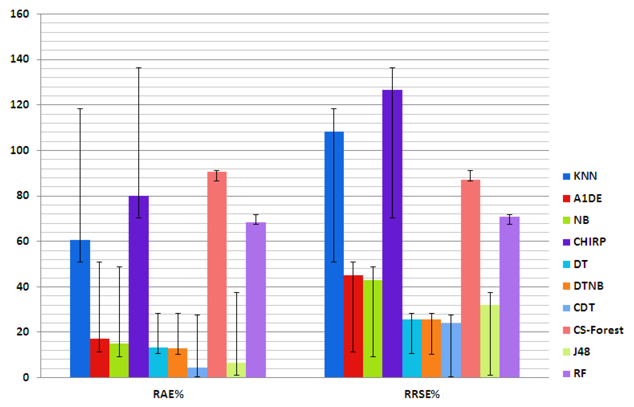
10	RF	0.191	0.265	68.211	70.995

shows the MAE, RMSE, RAE, and RRSE results accomplished via each individual technique. In the table, the second column represents the list of techniques while rest of the columns represent the error measures. The outcomes of this table show that CDT outperforms the other techniques by reducing the error rate. For better understanding, these analyses are also presented in Figure 3 and Figure 4, respectively, with standard deviation bar. Standard Deviation (SD) is a quantity of distribution of the data commencing the mean. It is a possession of the variable that bounces an impression of the assortment in which the values scatter (dispersal of the data). Error bars of ten symbolize one SD of indecision. The magnitudes are not the same and so the extent carefully chosen should be specified explicitly in the graph or supporting text. Archetypally, error bars are used to display the SD. The artless thing that we can do to enumerate variability is to calculate the SD. Essentially, this articulates us how much the values in each cluster incline to deviate from their mean.

5.2. Analysis Phase 2

In this phase, all accuracy measures are analyzed.

Table 26. Precision, Recall and F-Measure analysis of each employed technique.

S. No.	Technique	Precision	Recall	F-Measure
1	KNN	0.578	0.582	0.579
2	AIDE	0.910	0.906	0.907
3	NB	0.914	0.910	0.911
4	CHIRP	0.475	0.440	0.440
5	DT	0.980	0.980	0.980
6	DTNB	0.980	0.980	0.980
7	CDT	0.980	0.980	0.980
8	CS-Forest	0.772	0.732	0.699
9	J48	0.964	0.963	0.963
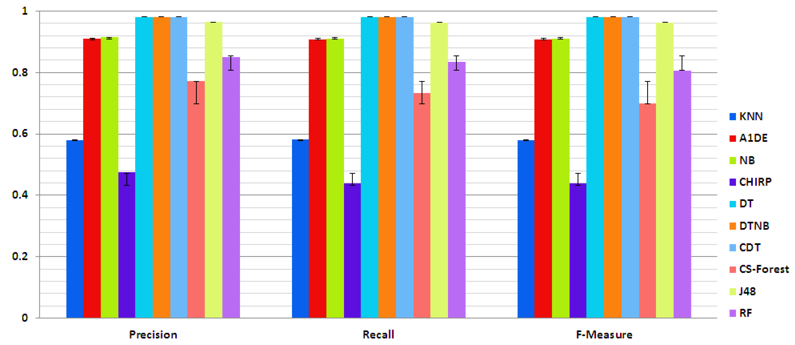
10	RF	0.851	0.833	0.805

presents the performance of each technique evaluated via precision, recall, and F-measure. In this table, the first column represents the evaluation measures while the second column represents the employed techniques. The rest of the columns in the table present the outcome of each individual technique evaluated through each measure. The outcomes show that DT, DTNB, and CDT beat the rest of the employed techniques and produce the same results with each evaluation measure, i.e., 0.980. For better understanding, these results are also presented in Figure 5 through columns and SD bars.

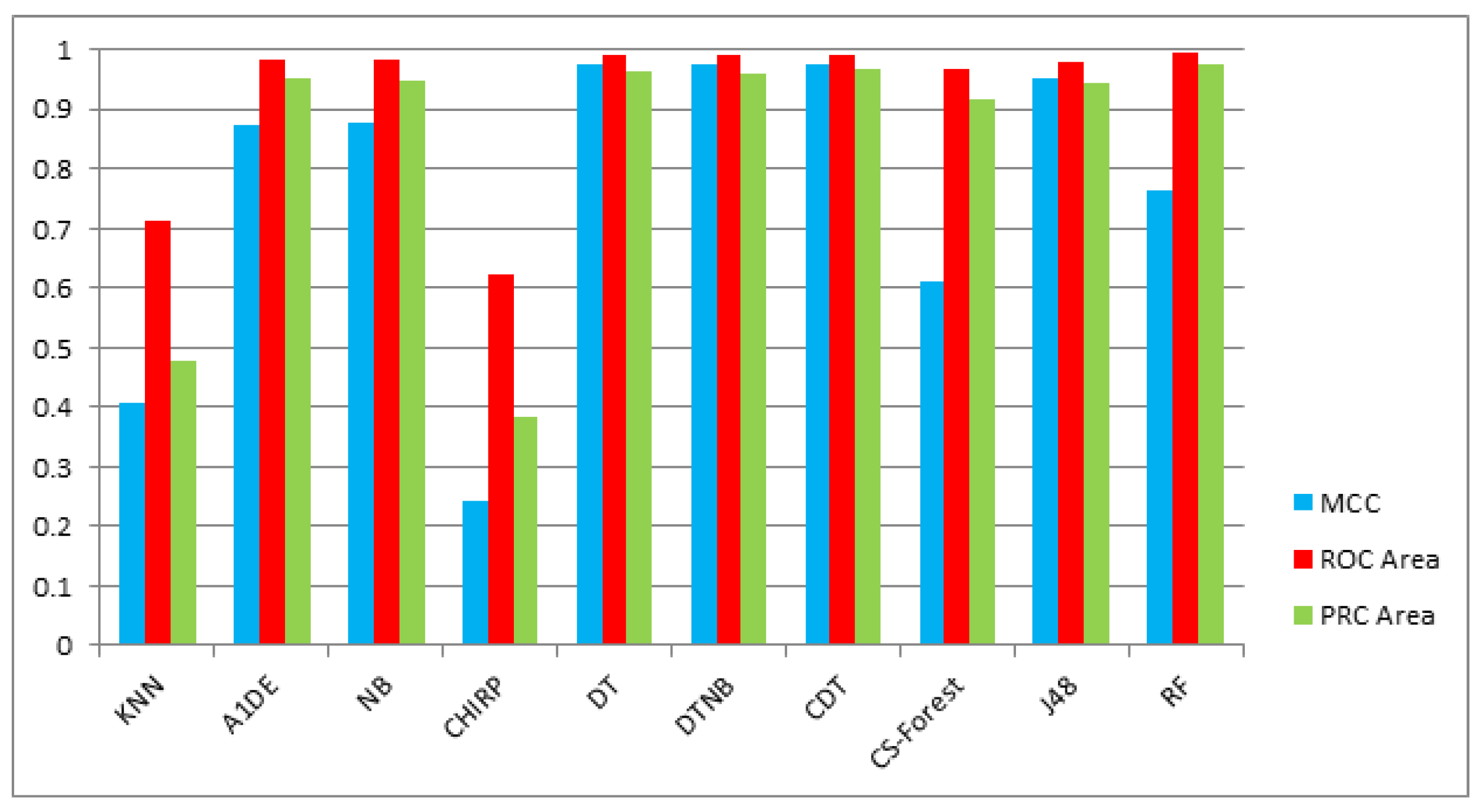
The evaluation through MCC, ROC area, and PRC area are presented in

Table 27. MCC, ROC Area and PRC Area analysis of each employed technique.

S. No.	Technique	MCC	ROC Area	PRC Area
1	KNN	0.406	0.713	0.476
2	AIDE	0.872	0.983	0.952
3	NB	0.877	0.982	0.947
4	CHIRP	0.243	0.624	0.385
5	DT	0.975	0.991	0.965
6	DTNB	0.975	0.991	0.959
7	CDT	0.975	0.990	0.968
8	CS-Forest	0.613	0.969	0.915
9	J48	0.952	0.981	0.945
10	RF	0.766	0.994	0.975

. These outcomes show that evaluating each technique through MCC, DT, DTNB and CDT outperforms the other techniques and generates the same results that is 0.975. However, On ROC area and PRC area RF outperforms other employed techniques and generates 0.994 and 0.975 results respectively for ROC area and PRC area. The columns in Figure 6 elaborates the analysis of this phase.

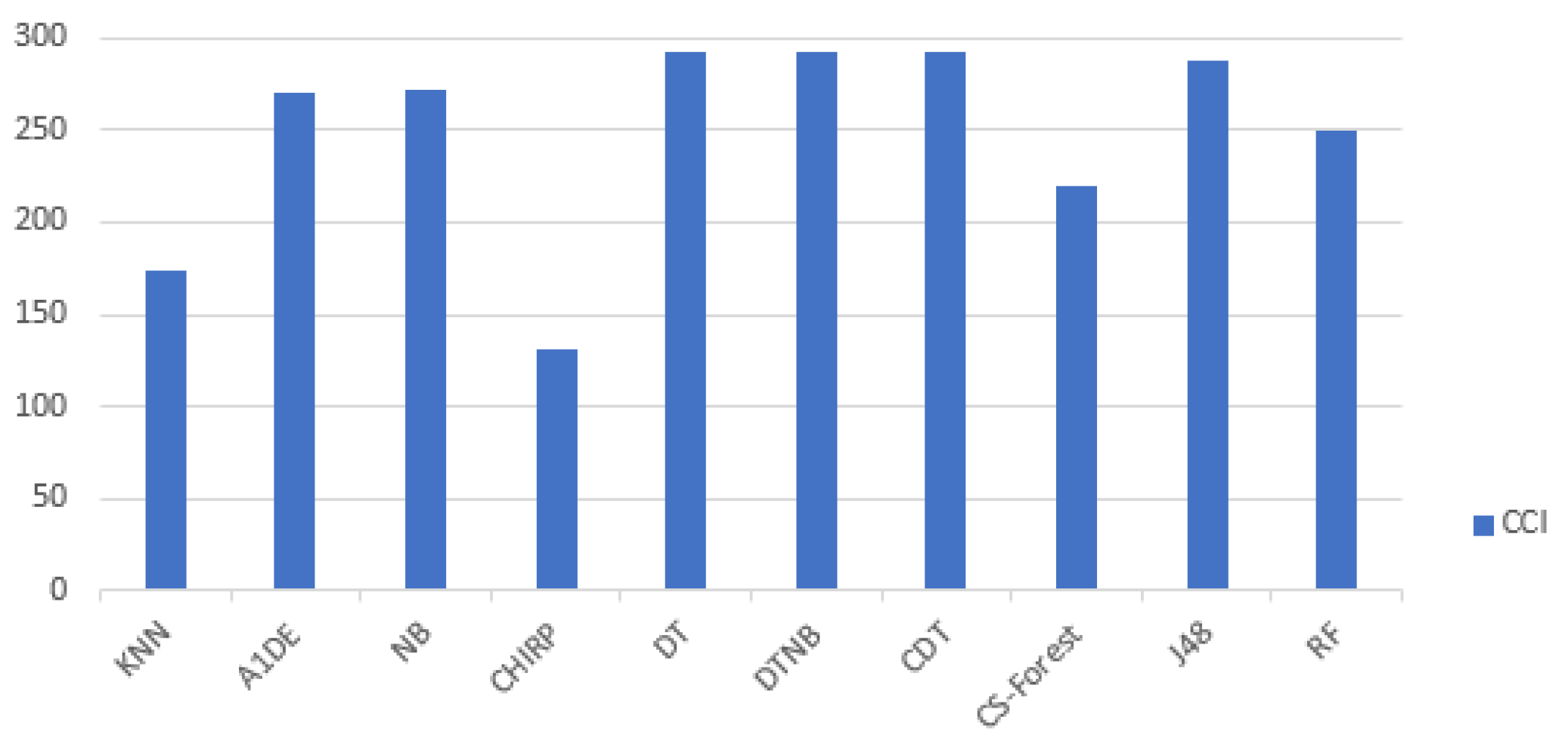
CCI is considered to be the accuracy of the individual employed technique. The dataset used in this research consists of a total of 299 instances.

Table 28. CCI Details out of 299 Instances.

S. No.	Technique	CCI	Accuracy%
1	KNN	174	58.194
2	AIDE	271	90.635
3	NB	272	90.970
4	CHIRP	131	43.960
5	DT	293	97.993
6	DTNB	293	97.993
7	CDT	293	97.993
8	CS-Forest	219	73.244
9	J48	288	96.321
10	RF	249	83.278

presents the list of all CCI achieved via each individual technique. In the table, the second column shows the list of all used techniques, third column represents the CCI details while fourth column shows the accuracy in percentage. The inclusive analysis of the table shows that DT, DTNB, and CDT beat all the other employed techniques in terms of achieving higher accuracy, which is 97.993% for DT, DTNB, and CDT. The CCI analysis are further shown in Figure 7 with the help of a bar chart for better understanding.

6. Conclusions and Future Research Directions

Requirement risk prediction is an active research area with increasing contributions from the research community. This research aims to explore ML techniques for the first time for the requirement risk predictions using new dataset. This research contributed as follows. Ten ML techniques were explored for requirements risk prediction. A detailed comparison of these techniques for the proposed model is performed.

Requirement risk prediction had found great impact on the success or failure of the software project. To overcome this issue, a new model was needed to predict the risk in the project early, therefore, a model and optimal classifier is proposed.

Ten different ML techniques are employed and compared in this research and evaluated for reducing error rates and increasing accuracy of the proposed model. Among all these techniques CDT performed well in terms of overall accuracy, higher CCI, Lower MAE, and RMSE. The experiment shows the results as 0.0126 for MAE, 0.089 for RMSE, 4.498% for RAE, and 23.741% for RRSE. The results achieved are 0.980 for precision, recall and F-measure, 0.975 for MCC, and 97.993% for accuracy. DT, DTNB, and CDT perform better using precision, recall, F-measure, MCC, and accuracy.

From the experiments conducted in this research, it was observed that CDT was found to have the lowest error rates that are MAE of 0.013, RMSE of 0.089, RAE of 4.498, and RRSE of 23.741. We also observed that CDT was found to be the best in terms of CCI, i.e., 293 and accuracy of 97.993%. These results show that CDT can claim to be the best suitable and optimal classifier for the prediction of software risks.

The comprehensive outcomes of this study can be used as a reference point for other researchers. Any assertion concerning the enhancement in prediction through any new model, technique or framework can be benchmarked and verified. Some future directions are also listed as the accuracy may further be improved by employing other classification and pre-processing techniques in the proposed model. Class imbalance matter ought to be committed on these datasets. Furthermore, to increase the enactment, feature selection and ensemble learning techniques should also be explored. This research can be further validated using different assessment measures such as Mean Magnitude of Relative Error (MMRE), PRED etc. The dataset contains 299 instances from four different sources which can be enhanced by new requirements from other software project sources. It may also bring new challenges in the prediction of risks at requirement gathering phase.

References

- Shaukat, Z.S.; Naseem, R.; Zubair, M. A dataset for software requirements risk prediction. In Proceedings of the 2018 IEEE International Conference on Computational Science and Engineering (CSE), Bucharest, Romania, 29–31 October 2018; pp. 112–118. [Google Scholar] [CrossRef]
- Dhlamini, J.; Nhamu, I.; Kaihepa, A. Intelligent risk management tools for software development. In Proceedings of the 2009 Annual Conference of the Southern African Computer Lecturers’ Association, Eastern Cape, South Africa, 29 June–1 July 2009; pp. 33–40. [Google Scholar] [CrossRef] [Green Version]
- Salih, H.A.; Ammar, H.H. Model-based resource utilization and performance risk prediction using machine learning Techniques. Int. J. Inform. Vis. 2017, 1, 101–109. [Google Scholar]
- The Standish Group. The Standish group: The chaos report. Am. J. Hypertens. 2014. [Google Scholar] [CrossRef]
- Williams, L. Project risks product-specific risks. J. Secur. NCSU 2004, 1, 1–22. [Google Scholar]
- Shaukat, Z.; Naseem, R.; Zubair, M. Software requirement risk prediction dataset. In Proceedings of the 2018 IEEE International Conference on Computational Science and Engineering (CSE), Bucharest, Romania, 29–31 October 2018. [Google Scholar] [CrossRef]
- Deng, Z.; Zhu, X.; Cheng, D.; Zong, M.; Zhang, S. Efficient kNN classification algorithm for big data. Neurocomputing 2016, 195, 143–148. [Google Scholar] [CrossRef]
- Abdar, M.; Zomorodi-Moghadam, M.; Das, R.; Ting, I.H. Performance analysis of classification algorithms on early detection of liver disease. Expert Syst. Appl. 2017, 67, 239–251. [Google Scholar] [CrossRef]
- Wilkinson, L.; Anand, A.; Tuan, D.N. CHIRP: A new classifier based on composite hypercubes on iterated random projections. In Proceedings of the 17th ACM SIGKDD International Conference on Knowledge Discovery and Data Mining, San Diego, CA, USA, 21–24 August 2011; pp. 6–14. [Google Scholar] [CrossRef]
- Kaur, J.; Sabo, T.; Baghla, S.; Sabo, T. Modified Decision Table Classifier By Using Decision Support and Confidence In Online Shopping Dataset. Int. J. Comput. Eng. Technol. 2017, 8, 83–88. [Google Scholar]
- Hall, M.; Frank, E. Combining Naive Bayes and Decision Tables. In Proceedings of the Twenty-First International Florida Artificial Intelligence Research Society Conference, Coconut Grove, FL, USA, 15–17 May 2008; pp. 318–319. [Google Scholar]
- Singh, A.; Jain, A. Cost-sensitive metaheuristic technique for credit card fraud detection. J. Inf. Optim. Sci. 2020, 41, 1319–1331. [Google Scholar] [CrossRef]
- Khan, B.; Naseem, R.; Muhammad, F.; Abbas, G.; Kim, S. An empirical evaluation of machine learning techniques for chronic kidney disease prophecy. IEEE Access 2020, 8, 55012–55022. [Google Scholar] [CrossRef]
- Geetha, R.; Sivasubramanian, S.; Kaliappan, M.; Vimal, S.; Annamalai, S. Cervical Cancer Identification with Synthetic Minority Oversampling Technique and PCA Analysis using Random Forest Classifier. J. Med. Syst. 2019, 43. [Google Scholar] [CrossRef]
- Heidari, A.A.; Faris, H.; Aljarah, I.; Mirjalili, S. An efficient hybrid multilayer perceptron neural network with grasshopper optimization. Soft Comput. 2019, 23, 7941–7958. [Google Scholar] [CrossRef]
- Cao, W.; Wang, X.; Ming, Z.; Gao, J. A review on neural networks with random weights. Neurocomputing 2018, 275, 278–287. [Google Scholar] [CrossRef]
- Papernot, N.; Mcdaniel, P.; Jha, S.; Fredrikson, M.; Celik, Z.B.; Swami, A. The limitations of deep learning in adversarial settings. In Proceedings of the 2016 IEEE European Symposium on Security and Privacy (EuroS&P), Saarbrucken, Germany, 21–24 March 2016; pp. 372–387. [Google Scholar] [CrossRef] [Green Version]
- Abiodun, O.I.; Jantan, A.; Omolara, A.E.; Dada, K.V.; Mohamed, N.A.E.; Arshad, H. State-of-the-art in artificial neural network applications: A survey. Heliyon 2018, 4, e00938. [Google Scholar] [CrossRef] [PubMed] [Green Version]
- Berrar, D. Cross-validation. Encycl. Bioinformat. Comput. Biol. ABC Bioinformat. 2018, 1–3, 542–545. [Google Scholar] [CrossRef]
- Wang, W.; Lu, Y. Analysis of the Mean Absolute Error (MAE) and the Root Mean Square Error (RMSE) in Assessing Rounding Model. IOP Conf. Ser. Mater. Sci. Eng. 2018, 324. [Google Scholar] [CrossRef]
- Shalev-Shwartz, S.; Ben-David, S. Understanding Machine Learning: From Theory to Algorithms; IOP Publishing Ltd.: Kuala Lampur, Malaysia, 2014; ISBN 9781107057135. [Google Scholar]
- Nassif, A.B.; Capretz, L.F.; Hill, R. Analyzing the non-functional requirements in the desharnais dataset for software effort estimation. arXiv 2014, arXiv:1405.1131. [Google Scholar]
- Raji, C.G.; Chandra, S.S.V. Graft survival prediction in liver transplantation using artificial neural network models. J. Comput. Sci. 2016, 16, 72–78. [Google Scholar] [CrossRef]
- Menzies, T.; Dekhtyar, A.; Distefano, J.; Greenwald, J. Problems with precision: A response to ‘Comments on “data mining static code attributes to learn defect predictors’”. IEEE Trans. Softw. Eng. 2007, 33, 637–640. [Google Scholar] [CrossRef] [Green Version]
- Tong, H.; Liu, B.; Wang, S. Software defect prediction using stacked denoising autoencoders and two-stage ensemble learning. Inf. Softw. Technol. 2018, 96, 94–111. [Google Scholar] [CrossRef]
- Jacob, S.; Raju, G. Software defect prediction in large space systems through hybrid feature selection and classification. Int. Arab J. Inf. Technol. 2017, 14, 208–214. [Google Scholar]
- Witten, I.H.; Frank, E.; Hall, M.A. Data Mining: Practical Machine Learning Tools and Techniques (Google eBook); Elsevier: Burlington, NJ, USA, 2011. [Google Scholar]
- Balogun, A.O.; Bajeh, A.O.; Orie, V.A.; Yusuf-asaju, A.W. Software defect rediction using ensemble learning: An ANP based evaluation method. J. Eng. Technol. 2018, 3, 50–55. [Google Scholar]
- Anand, A.; Wilkinson, L.; Tuan, D.N. An L-infinity norm visual classifier. In Proceedings of the Ninth IEEE International Conference on Data Mining (ICDM), Miami, FL, USA, 6–9 December 2009; pp. 687–692. [Google Scholar]
- Manjula, C.; Florence, L. Deep neural network based hybrid approach for software defect prediction using software metrics. Cluster Comput. 2019, 22, 9847–9863. [Google Scholar] [CrossRef]
- Boehm, B. Software risk management: Principles and practices. IEEE Softw. 1991, 8, 32–41. [Google Scholar] [CrossRef]
- Moores, T.T.; Champion, R.E.M.; Tong, K. A methodology for measuring the risk associated with a software. Australas. J. Inf. Syst. 1996, 4, 55–63. [Google Scholar]
- Nikam, S.S. A Comparative Study of Classification Techniques in Data Mining Algorithms. Int. J. Mod. Trends Eng. Res. 2017, 4, 58–63. [Google Scholar] [CrossRef]
- Picek, S.; Heuser, A.; Guilley, S. Template attack versus bayes classifier. J. Cryptogr. Eng. 2017, 7, 343–351. [Google Scholar] [CrossRef]
- Pham, B.T. A novel classifier based on composite hyper-cubes on Iterated random projections for assessment of landslide susceptibility. J. Geol. Soc. India 2018, 91, 355–362. [Google Scholar] [CrossRef]
- Bijalwan, V.; Kumar, V.; Kumari, P.; Pascual, J. KNN based machine learning approach for text and document mining. Int. J. Database Theory Appl. 2014, 7, 61–70. [Google Scholar] [CrossRef]
- Alasker, H.; Alharkan, S.; Alharkan, W.; Zaki, A.; Riza, L.S. Detection of kidney disease using various intelligent classifiers. In Proceedings of the 2017 3rd International Conference on Science in Information Technology (ICSITech), Bandung, Indonesia, 25–26 October 2017; pp. 681–684. [Google Scholar]
- Mantas, C.J.; Abellán, J. Credal decision trees in noisy domains. In Proceedings of the 22nd European Symposium on Artificial Neural Networks, Computational Intelligence and Machine Learning (ESANN 2014), Bruges, Belgium, 23–25 April 2014; pp. 683–688. [Google Scholar]
- He, Q.; Xu, Z.; Li, S.; Li, R.; Zhang, S.; Wang, N.; Pham, B.T.; Chen, W. Novel entropy and rotation forest-based credal decision tree classifier for landslide susceptibility modeling. Entropy 2019, 21, 106. [Google Scholar] [CrossRef] [Green Version]
- Siers, M.J.; Islam, M.Z. Cost sensitive decision forest and voting for software defect prediction. In Lecture Notes in Computer Science; Including Subseries Lecture Notes Artificial Intelligence and Lecture Notes Bioinformatics; Springer: Cham, Switzerland, 2014; Volume 8862, pp. 929–936. [Google Scholar]
- Dar, K.S.; Azmeen, S.M.U. Dengue fever prediction: A data mining problem. J. Data Min. Genom. Proteom. 2015, 6. [Google Scholar] [CrossRef] [Green Version]
- Nahar, N.; Ara, F. Liver disease prediction by using different decision tree techniques. Int. J. Data Min. Knowl. Manag. Process 2018, 8, 1–9. [Google Scholar] [CrossRef]
- Jin, H.; Kim, S.; Kim, J. Decision factors on effective liver patient data prediction. Int. J. Bio-Sci. Bio-Technol. 2014, 6, 167–178. [Google Scholar] [CrossRef]
- Carvajal, T.M.; Viacrusis, K.M.; Hernandez, L.F.T.; Ho, H.T.; Amalin, D.M.; Watanabe, K. Machine learning methods reveal the temporal pattern of dengue incidence using meteorological factors in metropolitan Manila, Philippines. BMC Infect. Dis. 2018, 18, 1–15. [Google Scholar] [CrossRef] [PubMed]
Figure 1.
Requirement risk prediction model.
Figure 2.
Proposed research framework.
Figure 3.
MAE and RMSE analysis of individual techniques along with SD Bar.
Figure 4.
RAE% and RRSE% analysis of individual techniques along with SD Bar.
Figure 5.
Precision, Recall and F-Measure analysis of individual technique along with SD Bar.
Figure 6.
MCC, ROC Area and PRC Area analysis of individual technique.
Figure 7.
CCI analysis of individual technique.