


1. Introduction
Focusing small-amplitude acoustic waves with an array of transducers is commonly achieved through time-delay focusing and is termed ‘transmit beamforming’ (Szabo Reference Szabo2014). There, time delays added to the signal on each transducer can create a spherical convergent wave. Varying the delay allows one to move the focus of the wave and use it for acoustic scanning in diagnostic ultrasound. Focusing of finite-amplitude waves at a fixed location has been achieved with a single transducer bonded to a spherically shaped surface. Baac et al. (Reference Baac, Ok, Maxwell, Lee, Chen, Hart, Xu, Yoon and Guo2012) and Lee et al. (Reference Lee, Ok, Guo and Baac2016) used negative optical lenses covered with a light-absorbing coating to generate high-numerical-aperture acoustic sources for the generation of shock waves of several hundred bar. Using arbitrarily shaped surfaces allows one to modify the focus and even the waveform. Chan, Hies & Ohl (Reference Chan, Hies and Ohl2016) and Melde et al. (Reference Melde, Mark, Qiu and Fischer2016) demonstrated that the waveform and location of the focus of acoustic waves can be altered with arbitrarily shaped surfaces using three-dimensional (3-D) printing. Yet for dynamically focusing shocks, e.g. for a photoacoustic scanner, the focus location must be variable.
Here we demonstrate time-delay focusing for transient finite-amplitude waves with a variable focus. For this, cylindrical shock waves are generated along a line with two pairs of sources centred around the acoustic axis. The shocks are focused at different spatial locations on the axis by properly timing their launch. We find and explain why the positions of constructive superposition are very different from those expected for linear waves travelling in homogeneous media due to the nonlinear interaction between the shocks.
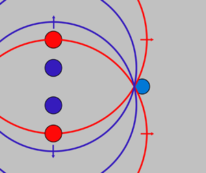
Transient time-delay focusing can be understood with an analogue to a binary Fresnel zone plate used in optics. Figure 1(a) shows one of those transmission masks, where the geometry of annular zones that transmit light is such that there is constructive interference at a location  $f$ on the
  $z$ axis. For the experiments in two dimensions, we take a linear cross-section of the mask (
 $yz$ axis in figure 1a) so that each ring is replaced by a pair of points where the transient excitation sources are created. However, in contrast to the optical case, our transient analogue has no restrictions on the position of the emitters because the constructive superposition is controlled by a time interval
  ${\rm \Delta} t$ between the sources. In a first realization, two internal (closest to the axis) and two external sources are used. Figure 1(b) depicts, at the top, the phase front for simultaneous launching
  ${\rm \Delta} t =0$ ns (plane wavefront, focus at infinity if no diffraction); in the middle, internal shocks created a few nanoseconds after the externals; and at the bottom, the case where the time difference is sufficient so that the overlap occurs near the origin (close to
  $z=0\ \mathrm {\mu }$m). Note that here we assumed linear superposition of the acoustic transient waves.

Figure 1. (a) Binary Fresnel zone plate. The experiment considers a two-dimensional analogue in the plane ( $yz$) where the emitter pairs are created on opposite sides of the
  $z$ axis. (b) Examples of focusing at different positions: simultaneous launching (
 ${\rm \Delta} t=0$ ns), and other cases with larger
  ${\rm \Delta} t$ resulting in overlap closer to the origin. (c) Simplified experimental set-up. (d) Geometry of the emitters on the
  $yz$ plane in the thin liquid gap.
2. Experimental set-up
To prove the concept, we have built an experiment based partly on previous work (Quinto-Su & Ando Reference Quinto-Su and Ando2013) but the illumination and excitation laser sources are exchanged. A simplified sketch of the experimental set-up is shown in figure 1(c). The acoustic transients are generated through photoacoustics (Lyamshev Reference Lyamshev1981; Wu, Frez & Diebold Reference Wu, Frez and Diebold2013) and generated by focusing two independent laser pulses (laser 1, laser 2) emitted from an Nd:YAG laser with two heads (Solo PIV, New Wave) with a wavelength of  $532$ nm and a pulse duration of
  $6$ ns. Conventionally, the two pulses are exciting the laser head collinearly, but we adjusted the outputs such that there is a finite angle between the directions of the two beams. In this way, after expanding both beams with a telescope, the collimated outputs are spatially separated by approximately
  $1$ cm when they reach the screen of the spatial light modulator (SLM, not shown). Because each laser pulse fills half the screen of the SLM, we can control the spatial phase for each of the beams with a single SLM. The beams are shaped by a two-dimensional (2-D) phase map obtained with the Gershberg–Saxon algorithm (Gerchberg & Saxton Reference Gerchberg and Saxton1972) focusing a single beam at two positions simultaneously. The laser pulses reflected from the SLM are focused and collimated with a pair of lenses before they are reflected with a dichroic mirror into the back aperture of the microscope objective (Olympus 10
 $\times$, numerical aperture 0.4).
The size of the beams at the back aperture of the microscope objective is approximately 2 mm, which results in a reduced effective numerical aperture of 0.05. Under those conditions, the diffraction-limited spot size of a focused Gaussian beam is  $2w_0 \sim 30 \ \mathrm {\mu }$m. Here the beam profile is not Gaussian, so the size of the focused spots is larger. In the numerical model, the size of the focused spots is an initial condition (along with initial pressure) that is optimized (starting with the size of a Gaussian beam as a lower bound) to fit the model to the measured individual shock dynamics.
The microscope objective focuses the beams into the container filled with an absorbing liquid for the laser wavelength (Epson printer ink, T6643 Magenta), which is an aqueous solution similar in viscosity and density to water. The liquid is bounded by a glass microscope slide and a thin glass coverslip (no. 1, 0.13–0.16 mm thick). The coverslip faces the microscope objective and the liquid gap height is approximately  $80\ \mathrm {\mu }$m, determined by the thickness of double sticky tape. Linear absorption of the focused laser pulses leads to stress confinement and the generation of an essentially cylindrical longitudinal wave from each focus.
The geometry of the focused spots is shown in figure 1(d); laser 1 focuses at the two central spots ( $y_1=\pm 75\ \mathrm {\mu }$m) while laser 2 focuses at the two outer spots (
 $y_2=\pm 145\ \mathrm {\mu }$m). The energy per spot is adjusted to
  $100 \pm 2\ \mathrm {\mu }$J so that the shock waves have nearly identical strength.
While measuring the pressure of the wave due to the experimental constraints is difficult, we utilize a stable gas bubble as a pressure sensor. This probe bubble is generated with a low-power continuous-wave (CW, 532 nm) laser heating the absorbing liquid creating a small gas bubble (radius  $R_0 \sim 15\text {--}30 \ \mathrm {\mu }$m) through local gas supersaturation. The CW laser beam is inserted into the optical path of the two laser pulses with a polarizing beamsplitter cube and is focused into the liquid sample through the same microscope objective. The bubble is placed on the
  $z$ axis at three positions,
  $z_1=64\ \mathrm {\mu }$m,
  $z_2=146\ \mathrm {\mu }$m and
  $z_3= 290\ \mathrm {\mu }$m. The events are imaged stroboscopically with a 6 ns pulse (Orion, New Wave,
  $\lambda =532$ nm converted to
  $690$ nm with a dye cell) and a charge-coupled device (CCD) camera (Sensicam QE, PCO). Other experiments use a
  $1\ \mathrm {\mu }$s laser pulse (637 nm, L637G1 Thorlabs) and are simultaneously imaged with a streak camera (SC-10, Optronis) and the CCD for single-shot collapse time measurements. Both red light sources are transmitted through the dichroic mirror of the microscope and focused close to a knife edge (lenses not shown) for schlieren photography.
Finally, the rather complex timing of all devices is realized with a programmable delay generator (Berkeley Nucleonics 575-8C).
3. Simulation
When the laser pulses arrive at the liquid sample, at each focused spot an acoustic wave is generated through stress confinement and a cavitation bubble by superheating the liquid through linear absorption (Vogel & Venugopalan Reference Vogel and Venugopalan2011). The shock wave is released once the expansion velocity of the vapour bubble reaches the local speed of sound. The vapour bubble dynamics is not important for the time-delay focusing because the gas–liquid interface velocity is considerably slower than the shock wave. Thus we use a single phase model, which is sufficient to model the acoustics of time-delay focusing.
The propagation and interaction between the shock waves is numerically modelled by employing the Mezcal code (De Colle & Raga Reference De Colle and Raga2005). This solver integrates the Euler equations with an equation of state for water on an adaptive mesh refinement grid (De Colle et al. Reference De Colle, Granot, López-Cámara and Ramirez-Ruiz2012). This resolves the shock while keeping computational costs sufficiently low (Veysset et al. Reference Veysset, Gutiérrez-Hernández, Dresselhaus-Cooper, De Colle, Kooi, Nelson, Quinto-Su and Pezeril2018). The employed equation of state (EOS) that relates thermal energy  $e_{th}$ and pressure
  $p$ is
  $e_{th} = ( p + \gamma p_\infty ) / (\gamma -1)$, with
  $p_\infty = 3.07 \times 10^8$ Pa and adiabatic index
  $\gamma = 7.15$ (Shyue Reference Shyue1998). We initialize the density by using the Tait EOS
  $\rho =\rho _0 [(p+p_\infty )/(p_0+p_\infty )]^{1/\gamma }$, with
  $p_0$ and
  $\rho _0$ being the water pressure and density at atmospheric pressure. This EOS is commonly used to model nearly incompressible flows (Tait Reference Tait1888).
The simulations are conducted on a 2-D Cartesian grid with size  $(x,y)=(-400,400)\ \mathrm {\mu }$m, with
  $400\times 400$ cells and four levels of refinement, corresponding to a minimum spatial resolution of
  $0.125\ \mathrm {\mu }$m. The domain is initialized with an ambient pressure of
  $10^5$ Pa and density of
  $10^3$ kg m
 $^{-3}$ except for the sites of shock wave emission, where the initial conditions are selected to fit the individual dynamics of the laser-induced shocks (
 $p_1=1.5$ GPa, radius
  $R_1=30\ \mathrm {\mu }$m,
  $\rho _1 =1.32 \rho _0$). Notice that the initial radius has twice the size of a calculated diffraction-limited spot size for a Gaussian beam. This is expected because aberrations and a non-Gaussian beam profile increase the size of the focused spots. The initial value of the pressure is consistent with those of laser-induced shocks with nanosecond lasers (Quinto-Su & Ando Reference Quinto-Su and Ando2013) at energies of the order of 100
  $\mathrm {\mu }$J.
4. Single pressure source
The experiments are done for the cases of individual shocks (internal/external), individual emitter pairs (internals/externals) and two pairs with  ${\rm \Delta} t =0, 15, 25$ and 35 ns. The dynamics are imaged with the 6 ns strobe. For all experimental results involving the four emitters (two externals, two internals), the outer shock waves are fired first at
  $t=0$ ns, while the inner shock waves at time
  $t={\rm \Delta} t$. We observe only the domain
  $z>0\ \mathrm {\mu }$m.
First, we measure the individual shock dynamics as a function of time  $R_{1,2}(t)$ (symbols in figure 2a). The continuous line in the figure is the simulated shock where the initial conditions (
 $R_1$ and
  $p_1$) were adjusted to fit the dynamics of the measured individual shocks.

Figure 2. (a) Individual shock dynamics. The symbols are the measurements and the continuous line represents the position of the simulated shock with an initial pressure of 1.5 GPa in a circle of radius  $30\ \mathrm {\mu }$m. (b) Pressures at different positions for an individual shock (simulated).
We observe that the speed of propagation is essentially constant with a speed of approximately  $1700$ m s
 $^{-1}$. With distance, this will drop to the acoustic speed of approximately
  $1500$ m s
 $^{-1}$, yet the slow decay is due to the effective 2-D geometry where the shock velocity in the liquid decays as
  $1/r$ (Veysset et al. Reference Veysset, Gutiérrez-Hernández, Dresselhaus-Cooper, De Colle, Kooi, Nelson, Quinto-Su and Pezeril2018), in contrast with the 3-D case that scales as
  $1/r^2$. Figure 2(b) shows the calculated maximum pressures at different radial distances. As expected, in the range of 0 to
  $30\ \mathrm {\mu }$m the maximum values are constant and equal to
  $p_1$.
5. Focusing for  ${\rm \Delta} t=15$ ns

In this section we discuss the particular delay of  ${\rm \Delta} t=15\ \textrm{ns}$ before we explore the dependence of the focusing for a range of delays between
  $0\le {\rm \Delta} t \le 35$ ns. The dynamics for
  ${\rm \Delta} t=15$ ns is shown in figure 3(a).

Figure 3. (a) Shock dynamics of the two pairs of emitters with  ${\rm \Delta} t=15$ ns (external pair launched at
  $t=0$ ns). The first row shows strobe photographs, while the second has the results of the simulation. The scale bar is 100
  $\mathrm {\mu }$m. The size of the individual frames is
  $413\ \mathrm {\mu }\textrm {m}\times 556\ \mathrm {\mu }$m. Overlap starting at 70 ns. Pressure bar in MPa. (b) Calculated maximum pressure on the axis.
The external shocks are created at  $t=0$ ns and they reach the high-pressure region for the internals at
  $t=15$ ns when the internal shocks are created, energizing them. At 30 ns (first image to the left) the shocks are expanding and the inner shocks are about to converge at
  $z=0\ \mathrm {\mu }$m. Later, at 70 ns, the inner and outer shocks are starting to overlap on the axis. We observe this overlap for times between 70 and 90 ns. The last frame is at 110 ns, where the shocks keep expanding. The simulation has reasonable agreement with the experiment. In the following section we discuss the general differences.
Figure 3(b) shows the calculated maximum pressure achieved on the axis ( $z>0\ \mathrm {\mu }$m) over the full simulation time of 200 ns. The four shocks overlap at
  $z=108\ \mathrm {\mu }$m at 68 ns, resulting in the highest pressure. We notice that near the maximum pressure there are small oscillations that appear due to a numerical artifact. This is produced because shock-capturing codes usually resolve a shock front with a few (three or four) cells. So, the pressure computed in each cell is an average over a region where pressures change quickly as the shock front propagates.
6. Focusing experiment
The results for the limiting cases of  ${\rm \Delta} t=0$ and 35 ns are shown in figure 4. In each case there is a direct comparison with the simulation.

Figure 4. Shock dynamics of the two pairs of emitters with different delay times. The second row are the results of the simulations. The scale bar is 100  $\mathrm {\mu }$m. Frame size of
  $413\ \mathrm {\mu }\textrm {m} \times 556\ \mathrm {\mu }$m. Pressure bar in MPa. (a)
  ${\rm \Delta} t=0$ ns. Overlap starting at
  $120$ ns. (b)
  ${\rm \Delta} t=35$ ns. Overlap starting at
  $60$ ns.
Figure 4(a) contains the case of  ${\rm \Delta} t=0$ ns, where all the emitters are injected at the same time. This would be equivalent to creating a planar wavefront. However, we observe that at 120 ns all the shocks have converged on the axis at
  $z=214\pm 20\ \mathrm {\mu }$m.
In the simulation, as the internal and external shocks have equal energies, they expand initially with the same speed. Thus, the internal shocks arrive at the symmetry axis first. The interaction of the two internal shocks increases the post-shock pressure, increasing the speed of the trailing external shocks and eventually resulting in superposition at  $z\sim 206\ \mathrm {\mu }$m. As the shocks cool by adiabatic expansion, the pressure drops with
  $z$ (figure 4a).
The overlap between the shocks gets closer to the axis origin as the time delay increases.
In particular, for  ${\rm \Delta} t =35$ ns (figure 4b), when the internal shocks are launched (at
  $t=35$ ns) they immediately overlap with the externals (50 ns). At 60 ns the shocks converge on the axis with the other internal/external pair very close to the origin at
  $z\sim 0\ \mathrm {\mu }$m.
Comparing the simulations with the experiments (figures 3 and 4) there are small discrepancies in the position and in the shape of the shocks. In the simulations the shock fronts appear to move slightly faster than in the experiment, but qualitatively the simulation yields similar results to the experiment even when we only consider the liquid component and a 2-D geometry. During interaction between the shocks, it is possible that the shock speed in the experiments decays a little faster than in the simulations. Also, in the simulation, during the first few tens of nanoseconds as the shocks propagate there is a negative pressure region (rarefaction) behind the shock fronts close to the source (for example, in the first frames in figures 3 and 4. When a shock reaches the vicinity of the other source, the tension slows down the shock, changing the shape of the shock front. In the experiment there is no tension at the location of the sources because of the expanding laser-induced cavitation bubbles. Overall, the results look very similar, even with the important differences of not simulating the bubbles and the deformation of the shock fronts in the simulation due to the negative pressure regions in the vicinity of the sources. Also, we have to consider that in the experiment the 6 ns exposure introduces some blurring compared with the instantaneous snapshot of the simulation.
7. Maximum pressures and position of acoustic focus
The calculated maximum pressures achieved on the axis are plotted in figure 5(a,b). The cases of two emitter pairs and individual shocks (external/internal) are shown in figure 5(a). As expected, in all cases the highest pressures are reached at the origin ( $z=0\ \mathrm {\mu }$m). The highest pressures are achieved for the case of two internal shocks in the range between 0 and
  $200\ \mathrm {\mu }$m. However, the pressure decay (as a function of
  $z$) for the two internal shocks is also the fastest. So for
  $z>200\ \mathrm {\mu }$m the pressure of the two external sources is slightly larger due to the slower decay. The individual sources both decay to similar values for large
  $z$.
$z$.

Figure 5. (a) Maximum pressures on the axis for single internal/external and pairs. (b) Maximum pressures on the axis for different delay times. (c) Focus position as a function of delay time. Circles extracted from (b). The continuous line is the position calculated from the dynamics of individual shocks  $R(t)$. Triangles with horizontal error bars are the measured positions of shock overlap.
The maximum pressures for the four emitters are shown in 5(b) for delay times  ${\rm \Delta} t$ between 0 and 35 ns in steps of 5 ns. We observe that, for simultaneous release of internal and external pairs (
 ${\rm \Delta} t =0$ ns), the internal shocks overlap first at
  $z=0\ \mathrm {\mu }$m where the maximum pressures are equal to those of the two internal sources (figure 5a); then the pressures decrease monotonically with increasing
  $z$. At
  $z\sim 160\ \mathrm {\mu }$m the external shocks start to catch up, increasing the pressure, with a local maximum achieved at
  $z\sim 206\ \mathrm {\mu }$m. This result is dramatically different from the expected planar wavefront for simultaneous launching where the external shocks would stay behind the internals near the axis. This is due to the nonlinear interaction between the shock waves, which leads to a speed increase of the external shocks when they interact with the wake of the internal shocks. In the linear model, on the other hand, the external and internal shock waves travel unperturbed. In the experiment near
  $z=0\ \mathrm {\mu }$m, the effect of the reflections should not be important, because only the internal shocks contribute to the maximum pressures.
The case of  ${\rm \Delta} t=5$ ns is similar, where shock focusing at large
  $z$ results in a noticeable pressure increase that is smaller than the pressure at
  $z=0\ \mathrm {\mu }$m. In all the other cases (
 ${\rm \Delta} t>5$ ns) the pressure increase at the acoustic focus are global maxima on the axis.
In general, for delay times  ${\rm \Delta} t$ between 0 and 20 ns, the maximum pressures before the acoustic focus are equal to those of the two internal shocks (figure 5a).
In the case of a delay time of 25 ns the pressure at the origin exceeds that of the two internal sources. For a time delay of 25 ns the maximum pressure at  $z=0\ \mathrm {\mu }$m is close to 1 GPa and has only a moderate increase during superposition. For
  ${\rm \Delta} t=35$ ns the shocks arrive at the origin simultaneously; the maximum pressure is larger than 1 GPa and stays almost constant in a range between 0 and
  ${\sim }80\ \mathrm {\mu }$m, decaying to values that are higher than or equal to the maxima achieved with the other delay times at their positions of constructive interference.
The dependence between focal positions and delay times is plotted in figure 5(c). The symbols (circles) are the results of the simulations (extracted from figure 5b), and the red triangles are the measured positions of convergence in the experiment; the uncertainty (horizontal error bars) represents the range of positions where we observe that overlap. The continuous line is calculated assuming that the shocks travel unperturbed in homogeneous media and considering the individual shock dynamics  $R(t)$ (figure 2a). The squared distance from each pair to an arbitrary focus on
  $z$ is
  $d_i^2 = y_i^2 + z^2$, where
  $y_i$ is the position of the emitters. Each excitation pair eventually converges at the
  $z$ axis at time
  $t_i(d_i)=R_i ^{-1}(d_i)$, where
  $R_i ^{-1}(r) =t(r)$ is the inverse function of
  $R_i(t)$. Considering that
  $y_i$ is fixed, then we can just write the time it takes for a shock
  $i$ (
$i$ ( $i=1,2$ internal/external) to reach
  $z$ as
  $t_i(z)$. If the external shocks are launched first (
 $t=0$ ns), then the internals have to start at a later time given by
  ${\rm \Delta} t (z)= t_2(z)- t_1(z)$. The plot of
  ${\rm \Delta} t (z)$ is the continuous line in figure 5(c). In the case for
  ${\rm \Delta} t=0$ ns, there is no overlap in the
  $300 \ \mathrm {\mu }$m range that we explore,and the expected delay time for convergence at
  $z=0\ \mathrm {\mu }$m is a little more than 40 ns, in contrast with the simulation and the experimental observations.
8. Pressure measurements
Measuring the pressure in a small liquid domain is a challenge. Variants of background oriented schlieren imaging have been used to measure laser-induced shocks in a domain of millimetres with maximum pressures of approximately  $2$ MPa (Hayasaka et al. Reference Hayasaka, Tagawa, Liu and Kameda2016). Here, we compare pressure ratios at three specific locations on the axis
  $z_i$ by measuring the collapse dynamics of a microscopic gas bubble with high temporal and spatial resolution. The shock-driven collapse of a bubble is shown in figure 6. The shock fronts reach the bubble at around
  $t=70$ ns; some of the wave is reflected as a rarefaction wave towards the left (
 $t=90$ ns) and the bubble starts to shrink. During collapse, that is, between
  $t=110$ ns and before
  $t=130$ ns, the emission of a shock wave from the bubble is visible. The bubble re-expands non-spherically, which can be explained by shock-induced jetting of the bubble (Ohl & Ikink Reference Ohl and Ikink2003; Supponen et al. Reference Supponen, Akimura, Minami, Nakajima, Uehara, Ohtani, Kaneko, Farhat and Sato2018).

Figure 6. Strobe images of shock-induced bubble collapse ( ${\rm \Delta} t = 35$ ns). Upon collapse, the bubble emits a shock wave (
 $t>110$ ns). The scale bar is 100
  $\mathrm {\mu }$m.
To determine the bubble dynamics and the collapse time with higher precision and in a single shot, streak imaging is used. Therefore, we replace the  $6$ ns laser illumination with a pulsed laser diode that has a pulse width of 1
 $\ \mathrm {\mu }$s. The events are imaged by both the CCD (blurred image) and the streak camera. Examples of those images are shown in figure 7, where the image at the left (figure 7a) is a streak image that we use to measure the collapse time in a single shot. The slit is the vertical direction in the streak readout image and the horizontal direction is time. The width of the streak image is 1
 $\ \mathrm {\mu }$s. Figure 7(b) shows the three positions of the jetting sensor bubble (
 $z_i= 64, 146, 290 \ \mathrm {\mu }$m).

Figure 7. (a) Streak image, slit centred on the axis ( $z$). Vertical scale bar (spatial) is 100 ns, horizontal scale bar (time) is 100
  $\mathrm {\mu }$m. (b) Blurred CCD images with the
  $1\ \mathrm {\mu }$s strobe showing the positions of the sensor bubble;
  $z_1=64\ \mathrm {\mu }$m,
  $z_2=146\ \mathrm {\mu }$m and
  $z_3= 290\ \mathrm {\mu }$m. Scale bar length is
  $200\ \mathrm {\mu }$m.
9. Collapse times
The interaction between a bubble and a shock wave has been studied extensively with simulations (Kapahi, Hsiao & Chahine Reference Kapahi, Hsiao and Chahine2015). Ignoring the shock reflection and for sufficiently long exposure to the pressure, the bubble collapse resembles the classical 3-D Rayleigh collapse  $T_{RC}$ (Rayleigh Reference Rayleigh1917):
 \begin{equation} T_{RC}=0.915 R_{0} \sqrt{\frac{\rho}{P_A}},\end{equation}
where  $P_A$ is the difference in pressure between the bubble interior and the surrounding liquid,
  $R_0$ is the radius of the probe bubble and
  $\rho$ is the liquid density.
In this experiment the bubbles are smaller than the height of the liquid container ( ${\sim }80\ \mathrm {\mu }$m), so the collapse is neither 2-D nor 3-D. However, the collapse time of these bubbles are proportional to the 3-D Rayleigh expression (Quinto-Su, Lim & Ohl Reference Quinto-Su, Lim and Ohl2009). Shock-induced collapses have also been shown to be proportional to the Rayleigh expression
  $R_0 \sqrt {\rho /P}$ (Kapahi et al. Reference Kapahi, Hsiao and Chahine2015). In this way, we can write the shock-induced collapse time as
 \begin{equation} T_{C} = \alpha R_{0} \sqrt{\frac{\rho}{P}} = m R_{0}. \end{equation}
The proportionality constant  $\alpha$ depends on the strength and duration of the shock and on the details of the collapse. Bourne & Field (Reference Bourne and Field1992) report proportionality constants with values between 1.17 and 0.62 for pressures in the range between 500 and 3500 MPa, respectively.
We performed our experiments by placing the sensor bubble at the three positions  $z_i$ on the axis and measured the collapse times for different conditions: single external/internal shock, external/internal pair and the four shocks with different time delays. For each event we measure the initial radius and the collapse time. We plot the ratios (
 $T_c/R_0$) as a function of
  $R_0$ for each event in figure 8. In this way, for each condition the ratios are centred around the constant value
  $m$.
$m$.

Figure 8. (a–c) Plots of  $(T_c/R_0)$ for different cases. One external/internal and two externals/internals at sensor bubble positions (a)
  $z_1$, (b)
  $z_2$ and (c)
  $z_3$. (d–f) Plots of (
 $T_c/R_0$) for all time delays. Sensor bubble at (d)
  $z_1$, (e)
  $z_2$ and (f)
  $z_3$.
The symbols are the ratios ( $T_C/R_0$) of the individual measurements, the continuous lines represent the average value
  $m$ and the shaded areas the standard deviations. The values of the mean and standard deviation are written next to the symbol in the figure legend.
The first column in figure 8 has the data for the sensor bubble placed at  $z_1$, which is the closest to the origin, while the second and third columns correspond to
  $z_2$ and
  $z_3$, respectively. The first row (figure 8a–c) has the cases for a single external/internal shock and the individual pairs interacting with the bubble. The second row (figure 8d–f) contains the cases for the two pairs of shocks with delays
  ${\rm \Delta} t$ with values of 0, 15, 25 and 35 ns.
Notice that smaller values of the ratios ( $T_C/R_0$) are a result of higher pressures, which decrease the collapse times. In this way the ratios increase monotonically with
  $z$ as the pressures decrease.
We can use the measurements of figure 8 to compare  $(T_C/R_0)$ ratios and estimate pressure ratios at the positions of the sensor bubble:
 \begin{equation} \frac{(T_C/R_0)_1}{(T_C/R_0)_2} \propto \sqrt{\frac{P_{2}}{P_{1}}}. \end{equation}
The relation is not exactly equal to the square root of the pressure ratios because each  $(T_C/R_0)$ ratio will have a different proportionality constant
  $\alpha$. However, we expect to be able to obtain a rough comparison between the pressures for different conditions, because the calculated maximum pressures (figure 5a,b) have a pressure range (maximum at
  $z_1$) between 177 MPa (one external shock) and 1050 MPa (four shocks with
  ${\rm \Delta} t=35$ ns). This pressure range is smaller than that reported by Bourne & Field (Reference Bourne and Field1992), and thus we expect to have less variations in the constants
  $\alpha$.
The comparison between the measured average ratios ( $T_C/R_0$) (figure 8) with the calculated square root of the pressure ratios at the same positions
  $z_i$ are given in tables 1 and 2. In all cases the ratios are compared with the case of
  ${\rm \Delta} t=35$ ns (at a given
  $z_i$), which represents some of the highest pressures along the axis. The various columns compare the measured
  $(T_C/R_0)$ ratios with the square root of the calculated pressures at
  $z_1$ to
  $z_3$.
Table 1. Comparison between measured  $(T_C/R_0)$ ratios (columns 2, 4 and 6) and calculated square root of pressure ratios (columns 3, 5 and 7) at
  $z_1$,
  $z_2$ and
  $z_3$. The ratios are extracted from figure 8(a–c) and the pressure ratios are from the simulations (figure 5a,b). The cases are compared with the maximum pressures of four emitters with
  ${\rm \Delta} t=35$ ns.

Table 2. Comparison between measured  $(T_C/R_0)$ ratios (columns 2, 4 and 6) and calculated square root of pressure ratios (columns 3, 5 and 7) at
  $z_1$,
  $z_2$ and
  $z_3$. The ratios are extracted from figure 8(d–f) and the pressure ratios are from the simulations (figures 5a,b). The cases are compared with the maximum pressures of four emitters with
  ${\rm \Delta} t=35$ ns.

Table 1 contains the comparisons with the cases for one internal/external and individual internal/external pairs, that is, it compares the highest pressures  ${\rm \Delta} t=35$ ns with the lowest pressure events at all the
  $z$ positions. This is where we would expect to have the highest discrepancies in the ratios because of the large differences in pressures.
Surprisingly, most of the measurements have a reasonable agreement with the square root of the calculated maximum pressure ratios (extracted from figure 5a,b). The cases where the square root of the pressure ratios fall outside the reported measurement intervals are for one external shock (at  $z_1$) (difference of
  $29\,\%$, considering the centre of the measured interval, and
  $12\,\%$, considering the lower bound) and for one internal shock (at
  $z_2$) (difference of
  $19\,\%$, considering the centre of the measured interval, and approximately
  $4\,\%$, considering the upper bound). The square roots comparing the calculated pressures for two external shocks at
  $z_1$ and
  $z_2$ are at the edge of the measured intervals.
Table 2 compares the cases for the four shocks at the three positions  $z_i$ with the case
  ${\rm \Delta} t =35$ ns. Here the difference between the maximum pressures (at
  ${\rm \Delta} t=35$ ns) and the other cases with different delay times are smaller than in table 1. The case where the square root of the pressure ratios lies outside the measured interval is that for
  ${\rm \Delta} t=0\ \textrm{ns}$ at
  $z_2$ with a difference of approximately
  $15\,\%$ considering the centre of the measured interval and approximately
  $2\,\%$ considering the upper bound of the measurement.
At the closest position  $z_1$, the pressures are the highest, and for
  ${\rm \Delta} t$ in the range between 0 and 20 ns the main contribution to the highest pressure is given by the two internal shocks, which is why the interaction between the external shocks and the internal bubbles do not affect the measurements. In the case of larger
  ${\rm \Delta} t$, the external shocks have passed the internal sources when these are created and there is no interaction with the bubbles, and have converged when reaching the sensor bubble. At
  $z_3$ all the shocks have converged into a single lower-pressure condition, and for
  ${\rm \Delta} t=0$ ns the sections that interacted with the bubble do not contribute. In the case of
  $z_2$, the bubble is exposed first to the internal shocks and a little later to the external shocks. This is not represented in figure 5(a,b) because there we plot the maximum pressure at each
  $z$. In the experiment the bubble collapses faster than would be expected by the pressure at that point because the internal shocks reach it first and a little later the external shocks arrive. In this way the maximum pressure at
  $z_2$ for that condition slightly underestimates the effective pressure that induces a faster collapse. However, the ratios are still consistent with the square roots of the calculated pressures.
10. Summary and conclusion
We have shown that the nonlinear interaction between the shocks is crucial to explain the results, where the regions of constructive interference are closer to the origin than expected in a homogeneous medium. The results are important for designing systems that focus high-pressure transient waves.
In our system, the highest pressures are attained for focus near the origin with  ${\rm \Delta} t= 35$ ns, resulting in almost constant pressure followed by decay. The pressures are comparable to those with precise overlap at all points on the axis. Delay times in the range of 10–30 ns achieve the highest pressure upon convergence; while for 0–5 ns the pressure increase is smaller than the pressure achieved during the initial overlap of the internal shocks.
At a delay time of 0 ns, the shocks converge at  $z\sim 206\ \mathrm {\mu }$m. In order to achieve overlap farther away, negative delay times are needed, that is, internal shocks launching first so that the external shocks catch up at longer
  $z$.
$z$.
Our collapse time measurements are used to estimate the square root of the calculated maximum pressure ratios for different conditions. The method yields reasonable results, despite the fact that there are constants that change with different conditions. The pressure ratio method is limited and does not give information about the absolute pressures that are reached. To validate absolute pressures, we would need a two-component simulation that takes into account shock reflection at the phase boundaries. Additionally, the interaction of the launched shock waves with the expanding vapour bubbles will affect the acoustic field after first focusing. Here, again, a two-component simulation is needed to account for their contribution. Johnsen & Colonius (Reference Johnsen and Colonius2006) and more recently Hawker & Ventikos (Reference Hawker and Ventikos2012), for example, have demonstrated that this kind of modelling is indeed feasible at least for the interaction of single shock waves.
Future work will include extending these results to three dimensions, where a pair of shocks will be replaced by a ring like in Veysset et al. (Reference Veysset, Gutiérrez-Hernández, Dresselhaus-Cooper, De Colle, Kooi, Nelson, Quinto-Su and Pezeril2018) in the  $yz$ plane and focusing will be achieved in the centre of the ring and along the vertical direction.
Acknowledgements
F.D.C. acknowledges the computing time granted by DGTIC UNAM (project LANCAD-UNAM-DGTIC-281).
Funding
This work was partially funded by DGAPA UNAM (IN107719, AG100820) and the Deutsche Forschungsgemeinschaft (DFG, OH 75/3-1).
Declaration of interests
The authors report no conflict of interest.


 Open access