Comparative Analysis of Climate Change Impacts on Meteorological, Hydrological, and Agricultural Droughts in the Lake Titicaca Basin


Abstract
:1. Introduction
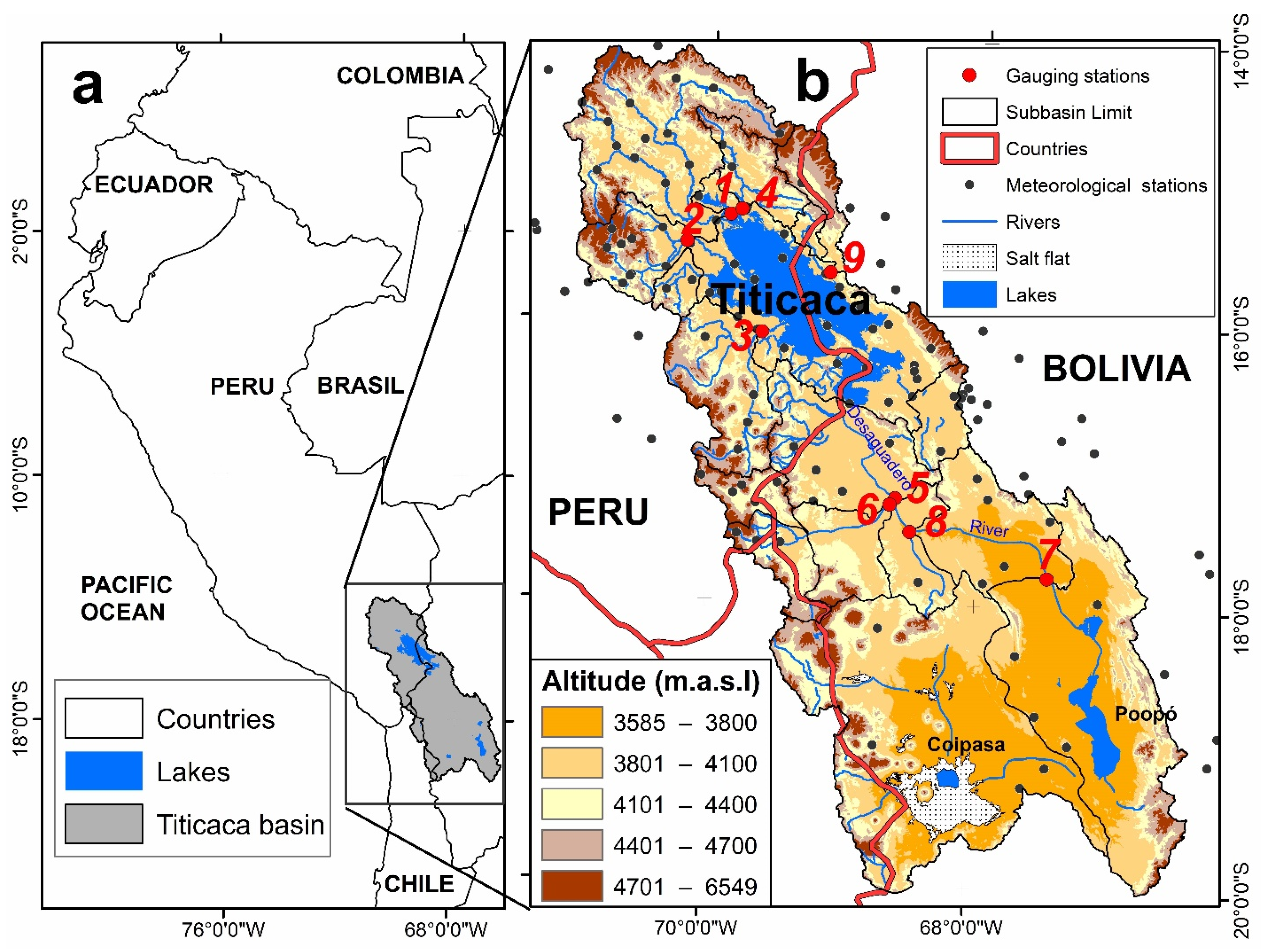
2. Study Area
3. Materials and Methods
3.1. Data
3.2. Methodology
3.2.1. Bias-Corrected Climate Projections and Selection of GCM Models
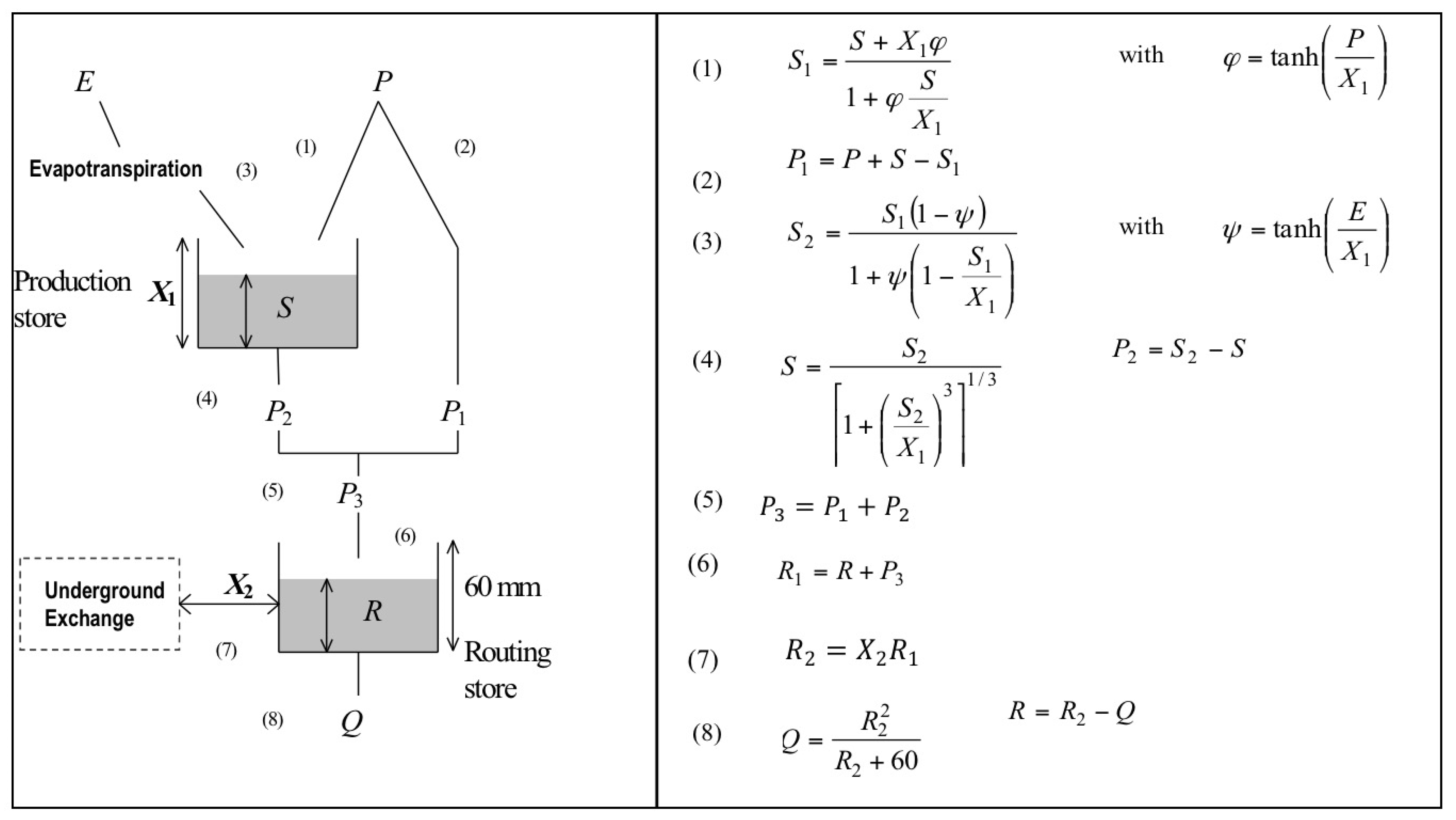
3.2.2. GR2M Model
3.2.3. Drought Analysis
SPI
SSMI
SRI
4. Results
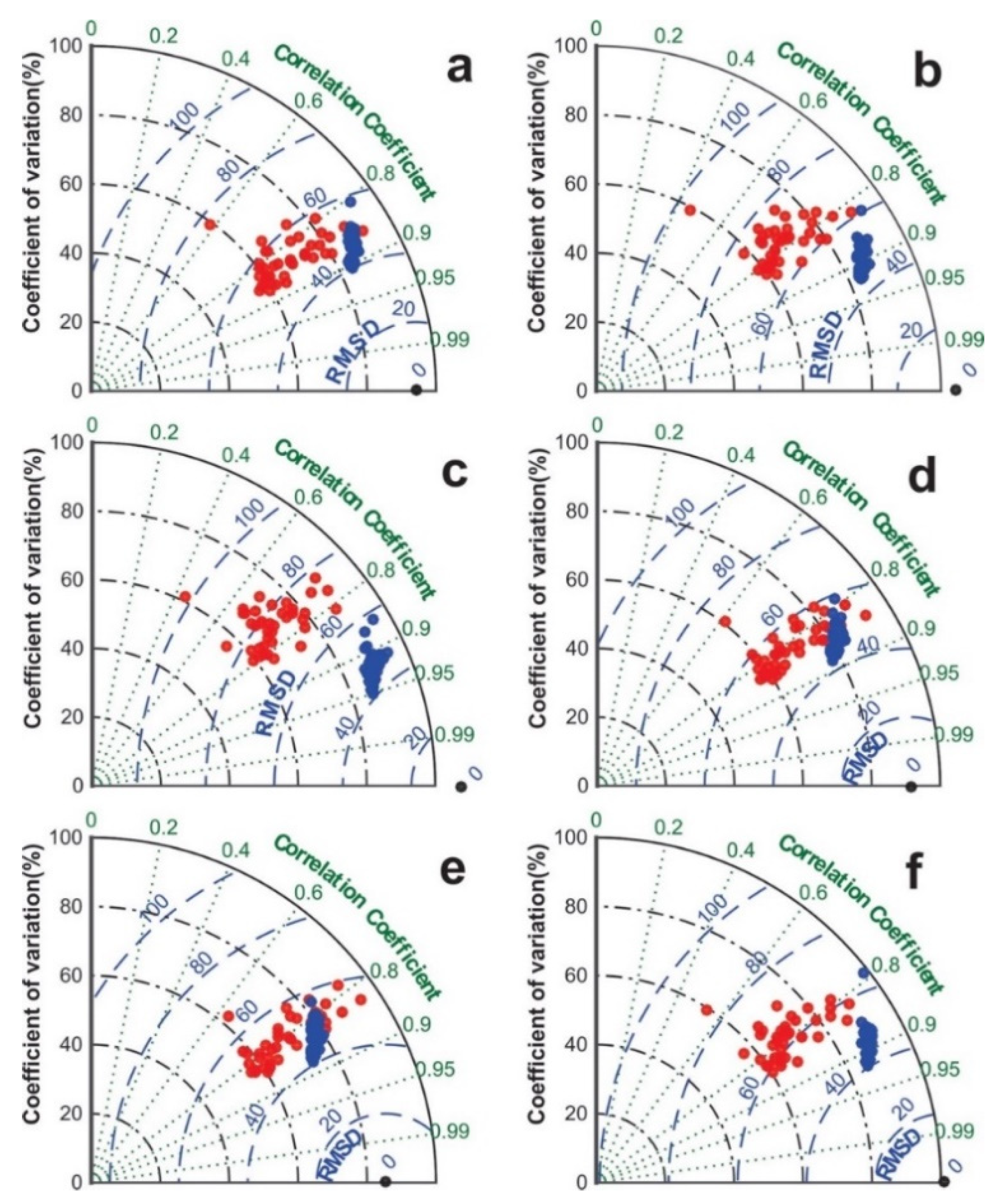
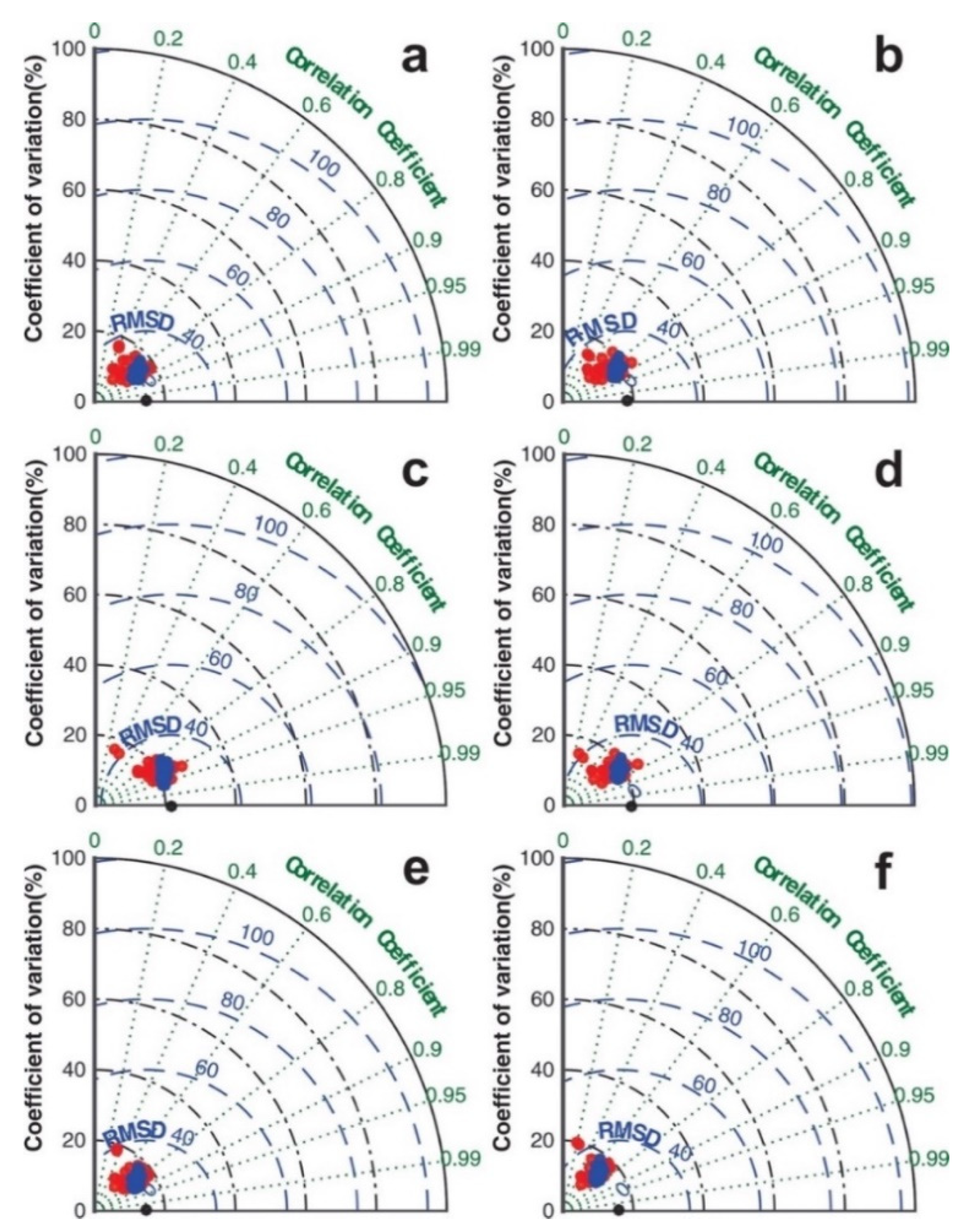
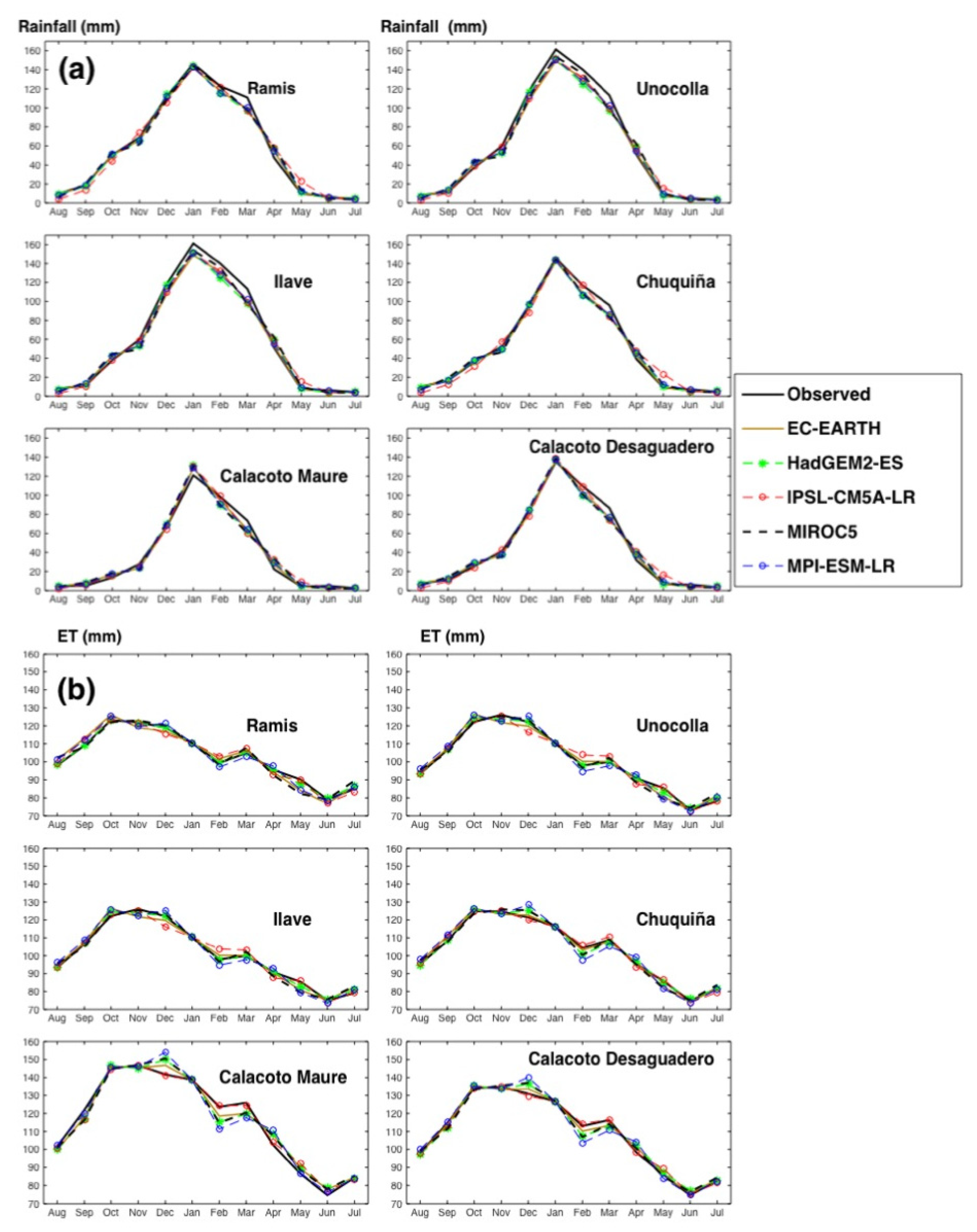
4.1. GCM Uncertainty Assessment
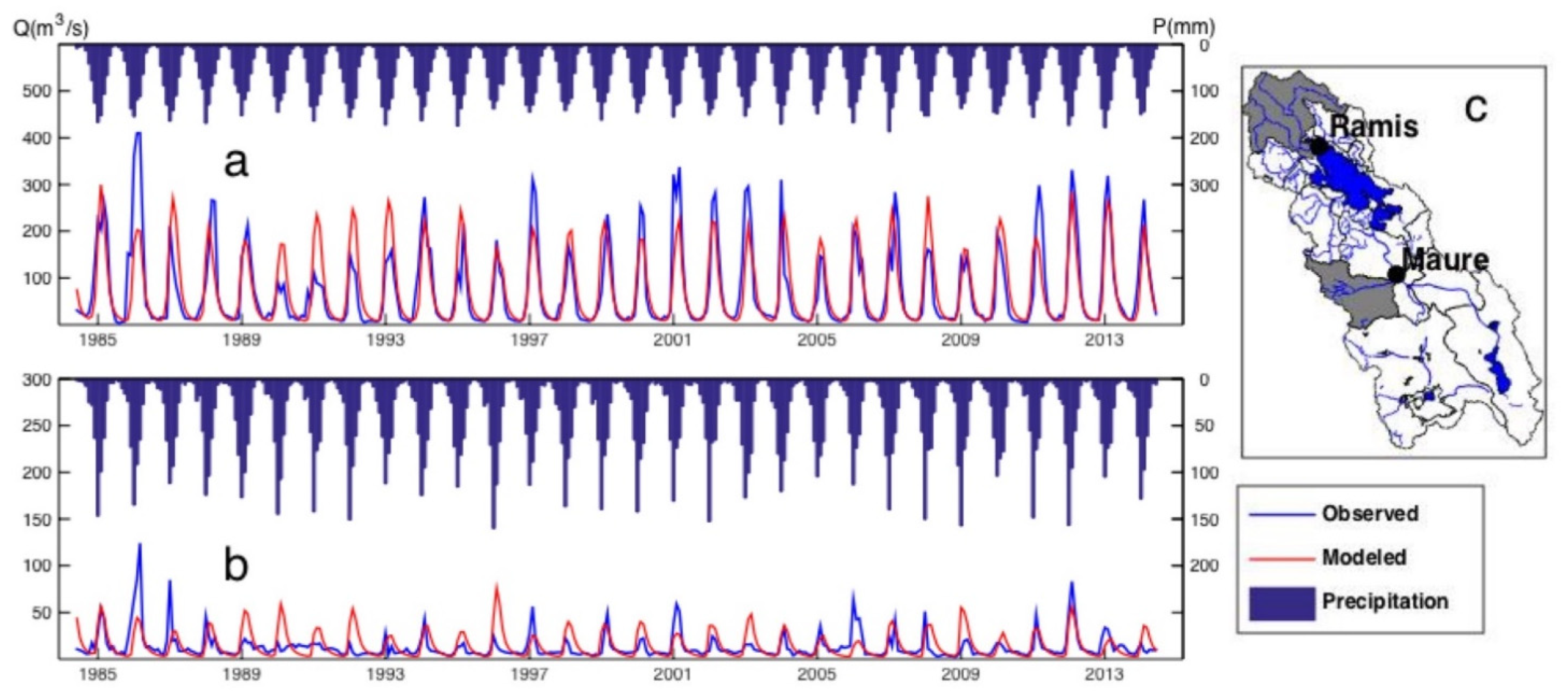
4.2. GR2M Model Performance
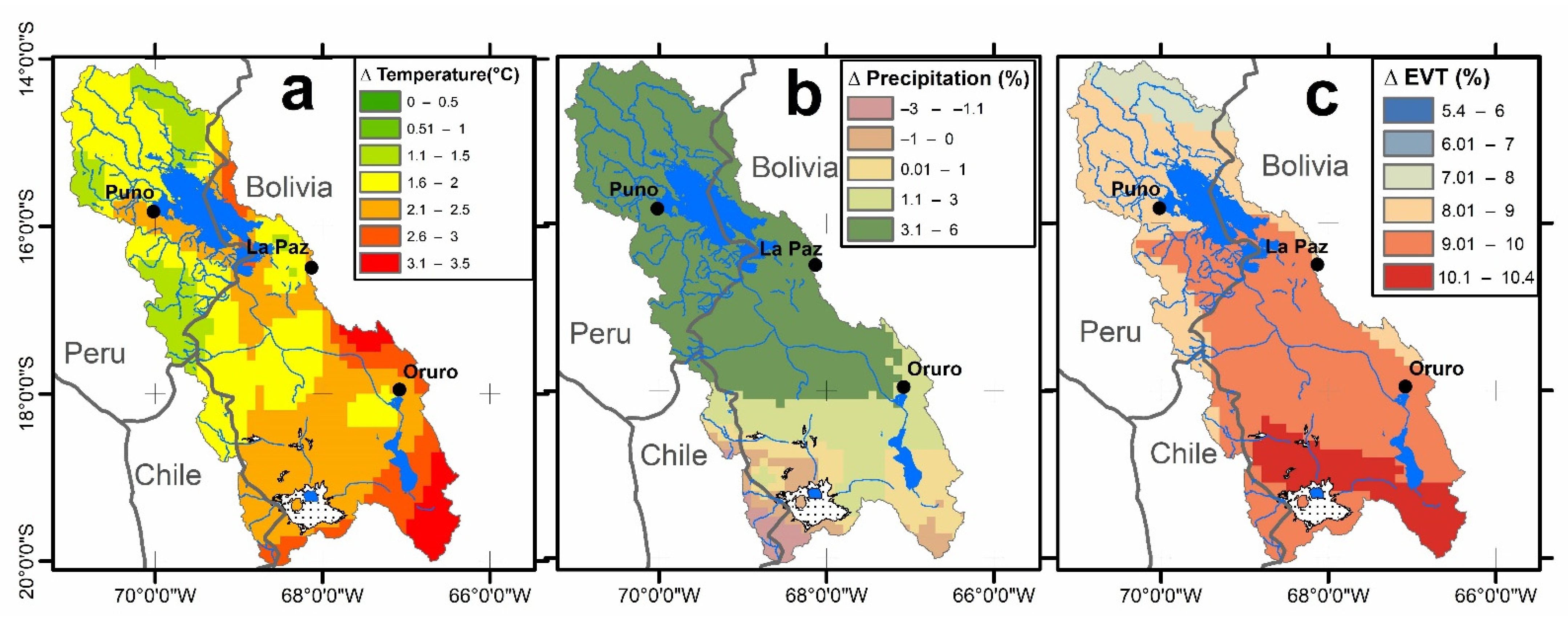
4.3. Spatial Distribution of Changes in Drought Characteristics
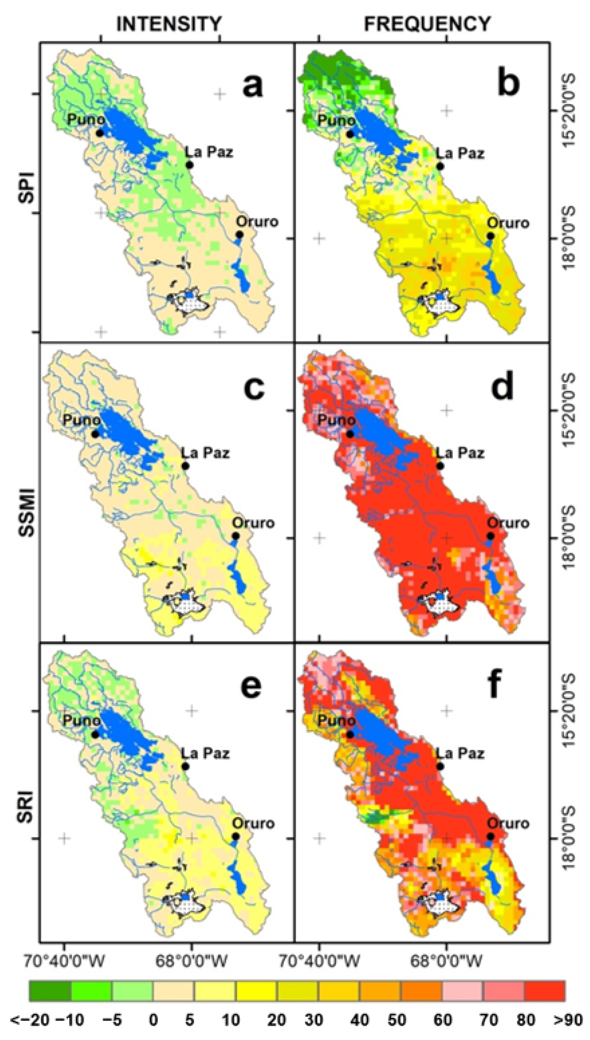
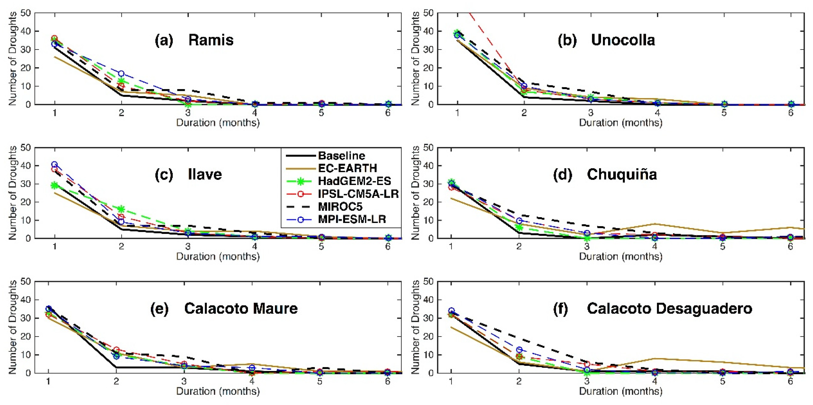
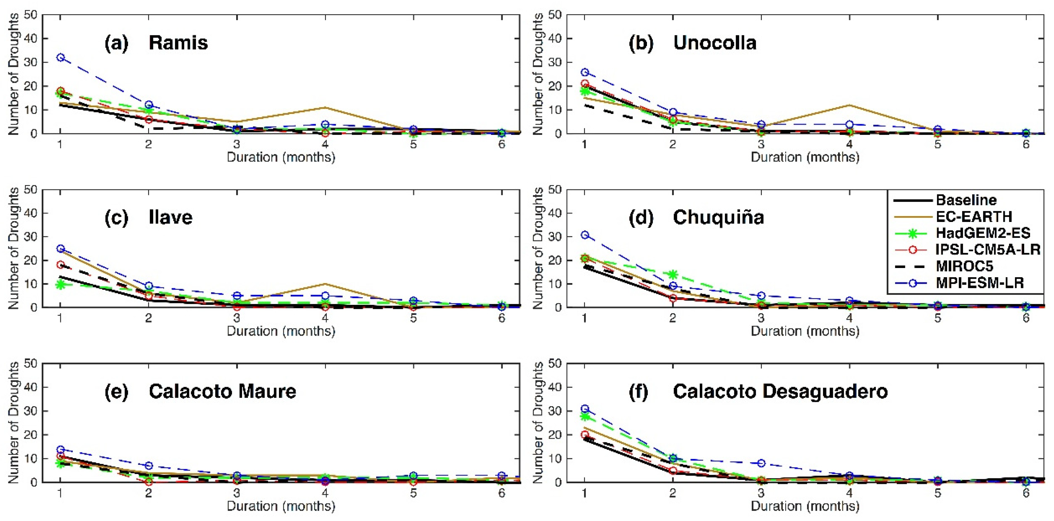
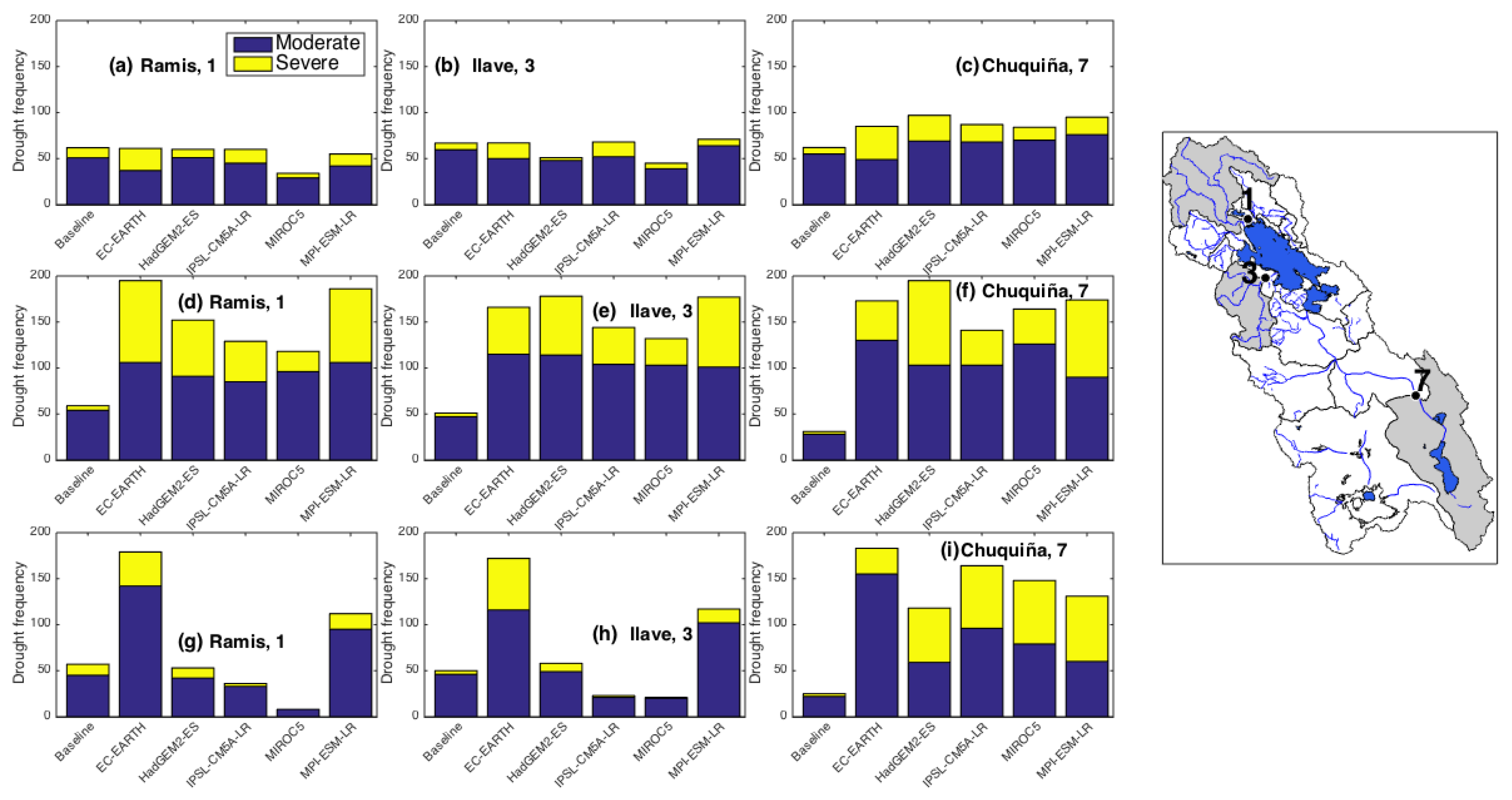
4.4. Changes in Drought Intensity, Duration, and Frequency
5. Discussion
6. Conclusions
Supplementary Materials
Author Contributions
Funding
Institutional Review Board Statement
Informed Consent Statement
Data Availability Statement
Acknowledgments
Conflicts of Interest
References
- Dai, A. Increasing drought under global warming in observations and models. Nat. Clim. Chang. 2012, 3, 52–58. [Google Scholar] [CrossRef]
- Van Loon, A.F.; Van Lanen, H.A.J. A process-based typology of hydrological drought. Hydrol. Earth Syst. Sci. 2012, 16, 1915–1946. [Google Scholar] [CrossRef] [Green Version]
- Mishra, A.K.; Singh, V.P. A review of drought concepts. J. Hydrol. 2010, 391, 202–216. [Google Scholar] [CrossRef]
- Duan, K.; Mei, Y. Comparison of meteorological, hydrological and agricultural drought responses to climate change and uncertainty assessment. Water Resour. Manag. 2014, 28, 5039–5054. [Google Scholar] [CrossRef]
- Liu, L.; Hong, Y.; Bednarczyk, C.N.; Yong, B.; Shafer, M.A.; Riley, R.; Hocker, J.E. Hydro-climatological drought analyses and projections using meteorological and hydrological drought indices: A case study in Blue River Basin, Oklahoma. Water Resour. Manag. 2012, 26, 2761–2779. [Google Scholar] [CrossRef]
- Leng, G.; Tang, Q.; Rayburg, S. Climate change impacts on meteorological, agricultural and hydrological droughts in China. Glob. Planet. Chang. 2015, 126, 23–24. [Google Scholar] [CrossRef]
- Sheffield, J.; Goteti, G.; Wen, F.; Wood, E.F. A simulated soil moisture based drought analysis for the United States. J. Geophys Res. 2004. [Google Scholar] [CrossRef]
- Mpelasoka, F.; Hennessy, K.; Jones, R.; Bates, B. Comparison of suitable drought indices for climate change impacts assessment over Australia towards resource management. Int. J. Climatol. 2008, 28, 1283–1292. [Google Scholar] [CrossRef]
- Hayes, M.J.; Alvord, C.; Lowrey, J. Drought indices. Intermt. West Clim. Summ. 2007, 3, 2–6. [Google Scholar]
- Zubieta, R.; Saavedra, M.; Silva, Y.; Giráldez, L. Spatial analysis and temporal trends of daily precipitation concentration in the Mantaro River basin: Central Andes of Peru. Stoch. Environ. Res. Risk Assess. 2016, 1–14. [Google Scholar] [CrossRef]
- Espinoza, J.C.; Ronchail, J.; Guyot, J.L.; Cocheneau, G.; Filizola, N.; Lavado, W.; de Oliveira, E.; Pombosa, R.; Vauchel, P. Spatio–Temporal rainfall variability in the Amazon Basin Countries (Brazil, Peru, Bolivia, Colombia and Ecuador). Int. J. Climatol. 2009, 29, 1574–1594. [Google Scholar] [CrossRef] [Green Version]
- Espinoza, J.C.; Ronchail, J.; Guyot, J.L.; Junquas, C.; Vauchel, P.; Lavado, W.S.; Drapeau, G.; Pombosa, R. Climate variability and extreme drought in the upper Solimões River (Western Amazon Basin): Understanding the exceptional 2010 drought. Geophys. Res. Lett. 2011. [Google Scholar] [CrossRef]
- Marengo, J.A.; Espinoza, J.C. Extreme seasonal droughts and floods in Amazonia: Causes, trends and impacts. Int. J. Climatol. 2015, 36, 1033–1050. [Google Scholar] [CrossRef]
- Mortensen, E.; Wu, S.; Notaro, M.; Vavrus, S.; Montgomery, R.; De Piérola, J.; Sánchez, C.; Block, P. Regression-based season-ahead drought prediction for southern Peru conditioned on large-scale climate variables. Hydrol. Earth Syst. Sci. 2018, 22, 287–303. [Google Scholar] [CrossRef] [Green Version]
- Rocha, A. El Mega-Niño 1982-83, “La Madre de Todos los Niños”. In Proceedings of the Second International Congress on “Obras de Saneamiento, Hidráulica, Hidrología y Medio Ambiente”, HIDRO 2007-ICG, Lima, Peru, 1 June 2007. [Google Scholar]
- TDPS. Diagnostico de Daños por Eventos Extremos. Sistema Hídrico del Lago Titicaca, Rio Desaguadero, Lago Poopo y Salar de Coipasa (Sistema TDPS). 1996. Available online: http://www.oas.org/usde/publications/Unit/oea31s/begin.htm (accessed on 18 June 2018).
- ANA. Las Condiciones de Sequía y Estrategias de Gestión en el Perú. Informe Nacional del Perú; Autoridad Nacional del Agua, Ministerio de Agricultura: Lima, Peru, 2010.
- Vicente-Serrano, S.; Chura, O.; López-Moreno, J.; Azorin-Molina, C.; Sanchez-Lorenzo, A.; Aguilar, E.; Moran-Tejeda, E.; Trujillo, F.; Martínez, R.; Nieto, J. Spatio-temporal variability of droughts in Bolivia: 1955–2012. Int. J. Climatol. 2014, 35, 3024–3040. [Google Scholar] [CrossRef] [Green Version]
- Satgé, F.; Espinoza, R.; Zolá, R.; Roig, H.; Timouk, F.; Molina, J.; Garnier, J.; Calmant, S.; Seyler, F.; Bonnet, M.P. Role of Climate Variability and Human Activity on Poopó Lake Droughts between 1990 and 2015 Assessed Using Remote Sensing Data. Remote Sens. 2017, 9, 218. [Google Scholar] [CrossRef] [Green Version]
- Winters, C. Impact of climate change on the poor in Bolivia. Glob. Major. 2012, 3, 33–43. [Google Scholar]
- Minvielle, M.; Garreaud, R.D. Projecting rainfall changes over the South American Altiplano. J. Clim. 2011, 24, 4577–4583. [Google Scholar] [CrossRef]
- Seiler, C.; Hutjes, W.R.; Kabat, P. Likely Ranges of Climate Change in Bolivia. J. Appl. Meteorol. Climatol. 2013, 52, 1303–1317. [Google Scholar] [CrossRef]
- Escurra, J.; Vázquez, V.; Cestti, R.; De Nys, E. Climate change impact on countrywide water balance in Bolivia. Reg. Environ. Chang. 2014, 14, 727–742. [Google Scholar] [CrossRef]
- Vuille, M.; Bradley, R.S.; Werner, M.; Keimig, F. 20th Century Climate Change in the Tropical Andes: Observations and Model Results. Clim. Chang. 2003, 59, 75. [Google Scholar] [CrossRef]
- López-Moreno, J.I.; Morán-Tejeda, E.; Vicente-Serrano, S.M.; Bazo, J.; Azorin-Molina, C.; Revuelto, J.; Sánchez-Lorenzo, A.; Navarro-Serrano, F.; Aguilar, E.; Chura, O. Recent temperature variability and change in the Altiplano of Bolivia and Peru. Int. J. Clim. 2015. [Google Scholar] [CrossRef] [Green Version]
- Urrutia, R.; Vuille, M. Climate change projections for the tropical Andes using a regional climate model: Temperature and precipitation simulations for the end of the 21st century. J. Geophys. Res. 2009, 114, D02108. [Google Scholar] [CrossRef]
- Segura, H.; Junquas, C.; Espinoza, J.C.; Vuille, M.; Jauregui, Y.R.; Rabatel, A.; Condom, T.; Lebel, T. New insights into the rainfall variability in the tropical Andes on seasonal and interannual time scales. Clim. Dyn. 2019, 1–22. [Google Scholar] [CrossRef]
- Valdivia, C.; Thibeault, J.; Gilles, J.L.; García, M.; Seth, A. Climate trends and projections for the Andean Altiplano and strategies for adaptation. Adv. Geosci. 2013, 33, 69–77. [Google Scholar] [CrossRef]
- Garreaud, R. Subtropical cold surges: Regional aspects and global signatures. Int. J. Climatol. 2001, 21, 1181–1197. [Google Scholar] [CrossRef]
- Lagos, P.; Silva, Y.; Nickl, E.; Mosquera, K. El Niño, Climate Variability and Precipitation Extremes in Perú. Adv. Geosci. 2008, 14, 231–237. [Google Scholar] [CrossRef] [Green Version]
- Lavado, W.; Espinoza, J.C. Impact of El Niño and La Niña events on Rainfall in Peru. Rev. Bras. Meteorol. 2014, 29, 171–182. [Google Scholar] [CrossRef] [Green Version]
- Canedo-Rosso, C.; Uvo, C.; Berndtsson, R. Precipitation variability and its relation to climate anomalies in the Bolivian Altiplano. Int. J. Climatol. 2018. [Google Scholar] [CrossRef] [Green Version]
- Segura, H.; Espinoza, J.C.; Junquas, C. Evidencing decadal and interdecadal hydroclimatic variability over the Central Andes. Environ. Res. Lett. 2016, 11–19. [Google Scholar] [CrossRef]
- Segura, H.; Espinoza, J.C.; Junquas, C.; Lebel, T.; Vuille, M.; Garreaud, R. Recent changes in the precipitation-driving processes over the southern tropical Andes/western Amazon. Clim. Dyn. 2020, 54, 2613–2631. [Google Scholar] [CrossRef]
- SENAMHI-Perú. Available online: www.senamhi.gob.pe (accessed on 12 March 2018).
- SENAMHI-Bolivia. Available online: http://senamhi.gob.bo (accessed on 15 June 2018).
- Hiez, G. L’ homogénéité des données pluviométriques. ORSTOM Ser. Hydrol. 1977, 14, 129–172. [Google Scholar]
- Brunet-Moret, Y. Homogénéisation des précipitations. Cah. ORSTOM Ser. Hydrol. 1979, 16, 3–4. [Google Scholar]
- Vauchel, P. Hydraccess: Software for Management and Processing of Hydro-Meteorological Data. 2005. Available online: https://hybam.obs-mip.fr/es/software/ (accessed on 1 May 2018).
- Riahi, K.; Krey, V.; Rao, S.; Chirkov, V.; Fischer, G.; Kolp, P.; Kindermann, G.; Nakicenovic, N.; Rafai, P. RCP-8.5: Exploring the consequence of high emission trajectories. Clim. Change 2011. [Google Scholar] [CrossRef] [Green Version]
- Buytaert, W.; Vuille, M.; Dewulf, A.; Urrutia, R.; Karmalkar, A.; Célleri, R. Uncertainties in climate change projections and regional downscaling in the tropical Andes: Implications for water resources management. Hydrol. Earth Syst. Sci. 2010, 14, 1247–1258. [Google Scholar] [CrossRef] [Green Version]
- Hempel, S.; Frieler, K.; Warszawski, L.; Schewe, J.; Piontek, F. A trend-preserving bias correction–the ISI-MIP approach. Earth Syst. Dynam. 2013, 4, 219–236. [Google Scholar] [CrossRef] [Green Version]
- SENAMHI-Peru. Statistical Downscaling of Climate Scenarios over Peru. Servicio Nacional de Meteorología e Hidrología. 2014. Available online: http://www.fao.org/3/a-bt558e.pdf (accessed on 18 September 2017).
- Hargreaves, G.H.; Samani, Z.A. Reference crop evapotranspiration from temperature. Trans. ASAE 1985, 2, 96–99. [Google Scholar] [CrossRef]
- Garcia, M.; Raes, D.; Jacobsen, S.E. Evapotranspiration analysis and irrigation requirements of quinoa (Chenopodium quinoa) in the Bolivian highlands. Agric. Water Manag. 2003, 60, 119–134. [Google Scholar] [CrossRef]
- Garcia, M.; Raes, D.; Allen, R.G.; Herbas, C. Dynamics of reference evapotranspiration in the Bolivian highlands (Altiplano). Agric. Water Manag. 2004, 125, 67–82. [Google Scholar] [CrossRef]
- Vacher, J.; Imaña, E.; Canqui, E. Las caracteristicas radiativas y la evapotranspiración potencial en el Altiplano boliviano. Revista Agricultura. Facultad de Ciencias Agricolas, Pecuarias, Forestales y Veterinarias. Univ. Mayor San Simon 1994, 24, 4–11. [Google Scholar]
- Laqui, W.; Zubieta, R.; Rau, P.; Mejía, A.; Lavado, W.; Ingol, E. Can artificial neural networks estimate potential evapotranspiration in Peruvian highlands? Model. Earth Syst. Environ. 2019, 5, 1911. [Google Scholar] [CrossRef]
- Lavado, C.W.; Labat, D.; Guyot, J.; Ardoin-Bardin, S. Assessment of climate change impacts on the hydrology of the Peruvian Amazon–Andes basin. Hydrol. Process. 2011, 25, 3721–3734. [Google Scholar] [CrossRef]
- Isaaks, E.H.; Srivastava, R.M. An Introduction to Applied Geostatistics; Oxford University Press: Oxford, UK, 1989. [Google Scholar]
- Parker, J.A.; Kenyon, R.V.; Troxel, D.E. Comparison of interpolating methods for image resampling. IEEE Trans. Med. Imaging 1983, 2, 31–39. [Google Scholar] [CrossRef] [PubMed]
- Roy, D.; Dikshit, O. Investigation of image resampling effects upon the textural information content of ahigh spatial resolution remotely sensed image. Int. J. Remote Sens. 1994, 15, 1123–1130. [Google Scholar] [CrossRef]
- Zorita, E.; Von Storch, H. The analog method as a simple statistical downscaling technique: Comparison with more complicated methods. J. Clim. 1999, 12, 2474–2489. [Google Scholar] [CrossRef]
- Piani, C.; Weedon, G.P.; Best, M.; Gomes, S.M.; Viterbo, P.; Hagemann, S.; Haerter, J.O. Statistical bias correction of global simulated daily precipitation and temperature for the application of hydrological models. J. Hydrol. 2010, 395, 199–215. [Google Scholar] [CrossRef]
- Taylor, K.E. Summarizing multiple aspects of model performance in a single diagram. J. Geophys. Res. 2001, 106, 7183–7192. [Google Scholar] [CrossRef]
- Satgé, F.; Ruelland, D.; Bonnet, M.P.; Molina, J.; Pillco, R. Consistency of satellite-based precipitation products in space and over time compared with gauge observations and snow-hydrological modelling in the Lake Titicaca region. Hydrol. Earth Syst. Sci. 2019, 23, 595–619. [Google Scholar] [CrossRef] [Green Version]
- Sterl, A.; Bintanja, R.; Brodeau, L.; Gleeson, E.; Koenigk, T.; Schmith, T.; Semmler, T.; Severijns, C.; Wyser, K.; Yang, S. A look at the ocean in the EC-Earth climate model. Clim. Dyn. 2012, 39, 2631. [Google Scholar] [CrossRef]
- Martin, G.M.; Bellouin, N.; Collins, W.J.; Culverwell, I.D.; Halloran, P.R.; Hardiman, S.C.; Hinton, T.J.; Jones, C.D.; McDonald, R.E.; McLaren, A.J.; et al. The HadGEM2 family of Met Office Unified Model climate configurations. Geosci. Model Dev. 2011, 4, 723–757. [Google Scholar] [CrossRef] [Green Version]
- Marti, O.; Braconnot, P.; Dufresne, J.L.; Bellier, J.; Benshila, R.; Bony, S.; Brockmann, P.; Cadule, P.; Caubel, A.; Codron, F.; et al. Key features of the IPSL ocean atmosphere model and its sensitivity to atmospheric resolution. Clim. Dyn. 2010, 34, 1–26. [Google Scholar] [CrossRef]
- Watanabe, M.; Suzuki, T.; O’ishi, R.; Komuro, Y.; Watanabe, S.; Emori, S.; Takemura, T.; Chikira, M.; Ogura, T.; Sekiguchi, M.; et al. Improved climate simulation by MIROC5: Mean states, variability, and climate sensitivity. J. Clim. 2010. [Google Scholar] [CrossRef]
- Giorgetta, M.A.; Jungclaus, J.; Reick, C.H.; Legutke, S.; Bader, J.; Böttinger, M.; Brovkin, V.; Crueger, T.; Esch, M.; Fieg, K.; et al. Climate and carbon cycle changes from 1850 to 2100 in MPI-ESM simulations for the Coupled Model Intercomparison Project phase 5. J. Adv. Modeling Earth Syst. 2013. [Google Scholar] [CrossRef]
- Niel, H.; Paturel, J.E.; Servat, E. Study of parameter stability of a lumped hydrologic model in a context of climatic variability. J. Hydrol. 2003, 278, 213–230. [Google Scholar] [CrossRef]
- Makhlouf, Z.; Michel, C. A two-parameter monthly water balance model for French watersheds. J. Hydrol. 1994, 162, 299–318. [Google Scholar] [CrossRef]
- Zubieta, R.; Laqui, W.; Lavado, W. Modelación hidrológica de la cuenca del río Ilave a partir de datos de precipitación observada y de satélite, periodo 2011–2015, Puno, Perú. Tecnol. Cienc. Agua. 2018, 9, 85–105. [Google Scholar] [CrossRef]
- Cruz, A.; Romero, J. Análisis Comparativo de los Modelos Lluvia-Escorrentía: GR2M, TEMEZ y LUTZ-SCHOLZ Aplicados en la Subcuenca del río Callazas; Universidad Peruana de Ciencias Aplicadas (UPC): Lima, Peru, 2018. [Google Scholar]
- Suarez, W.; Chevallier, P.; Pouyaud, B.; Lopez, P. Modelling the water balance in the glacierized Parón Lake basin (White Cordillera, Peru)/Modélisation du bilan hydrique du bassin versant englacé du LacParón (Cordillère Blanche, Pérou). Hydrol. Sci. J. 2008, 53, 266–277. [Google Scholar] [CrossRef] [Green Version]
- Mena Correa, S.P. Evolución de la Dinámica de los Escurrimientos en Zonas de Alta Montaña: Caso del Volcán Antisana. Tesis. Lic en Ing. Ambiental; Escuela Politécnica Nacional: Quito, Ecuador, 2010. [Google Scholar]
- Lamprea, Y. Estudio Comparativo de Modelos Multiparamétricos de Balance Hídrico a Nivel Mensual en Cuencas Hidrográficas de Cundinamarca y Valle del Cauca. Presentado Como Requisito Parcial Para Obtener el Título de Ingeniero Civil; Pontificia Universidad Javeriana: Bogotá, Colombia, 2011. [Google Scholar]
- Ma, X.; Lacombe, G.; Harrison, R.; Xu, J.; van Noordwijk, M. Expanding Rubber Plantations in Southern China: Evidence for Hydrological Impacts. Water 2019, 11, 651. [Google Scholar] [CrossRef] [Green Version]
- Yon, S.W.; King, K.; Polpanich, O.U.; Lacombe, G. Assessing hydrologic changes across the Lower Mekong Basin. J. Hydrol. Reg. Stud. 2017. [Google Scholar] [CrossRef]
- Lespinas, F.; Ludwig, W.; Heussner, S. Hydrological and climatic uncertainties associated with modeling the impact of climate change on water resources of small Mediterranean coastal rivers. J. Hydrol. 2014, 511, 403–422. [Google Scholar] [CrossRef]
- Meyer, S.; Blaschek, M.; Duttmann, R.; Ludwig, R. Improved hydrological model parametrization for climate change impact assessment under data scarcity—the potential of field monitoring techniques and geostatistics. Sci. Total Environ. 2016, 543, 906–923. [Google Scholar] [CrossRef] [PubMed]
- Hadour, A.; Mahé, G.; Meddi, M. Watershed based hydrological evolution under climate change effect: An example from North Western Algeria. J. Hydrol. Reg. Stud. 2020, 28, 100671. [Google Scholar] [CrossRef]
- Coulibaly, N.; Coulibaly, T.J.H.; Mpakama, Z.; Savané, I. The Impact of Climate Change on Water Resource Availability in a Trans-Boundary Basin in West Africa: The Case of Sassandra. Hydrology 2018, 5, 12. [Google Scholar] [CrossRef] [Green Version]
- Fathi, M.M.; Awadallah, A.G.; Abdelbaki, A.M.; Haggag, M.A. A new Budyko framework ex-tension using time series SARIMAX model. J. Hydrol. 2020, 570, 827–838. [Google Scholar] [CrossRef]
- Lacombe, G.; Ribolzi, O.; de Rouw, A.; Pierret, A.; Latsachak, K.; Silvera, N.; Pham Dinh, R.; Orange, D.; Janeau, J.-L.; Soulileuth, B.; et al. Contradictory hydrological impacts of afforestation in the humid tropics evidenced by long-term field monitoring and simulation modelling. Hydrol. Earth Syst. Sci. 2016, 20, 2691–2704. [Google Scholar] [CrossRef] [Green Version]
- Edijatno, E.; Michel, C. Un modèle pluie–débit journalier à trois paramètres. La Houille Blanch. 1989, 2, 113–121. [Google Scholar] [CrossRef] [Green Version]
- Duan, Q.; Sorooshian, S.; Gupta, V. Effective and efficient global optimization for conceptual rainfall-runoff models. Water Resour. Res. 1992, 28, 1015–1031. [Google Scholar] [CrossRef]
- Metropolis, N.; Rosenbluth, A.W.; Rosenbluth, M.N.; Teller, A.H.; Teller, E. Equation of state calculations by fast computing machines. J. Chem. Phys. 1953, 21, 1087–1092. [Google Scholar] [CrossRef] [Green Version]
- McKee, T.B.; Doesken, N.J.; Kliest, J. The relationship of drought frequency and duration to time scales. In Proceedings of the 8th Conference of Applied Climatology, Anaheim, CA, USA, 17–22 January 1993. [Google Scholar]
- Guennag, G.M.; Kamga, F.M. Computation of the Standardized precipitation index (SPI) and its use to assess drought occurrences in Cameroon over recent decades. J. Appl. Meterol. Climatol. 2014, 53, 2310–2324. [Google Scholar] [CrossRef]
- Hao, Z.; AghaKouchak, A. Multivariate standardized drought index: A parametric multi-index model. Adv. Water Resour. 2013, 57, 12–18. [Google Scholar] [CrossRef] [Green Version]
- Wang, A.; Lettenmaier, D.P.; Sheffield, J. Soil moisture drought in China, 1950–2006. J. Clim. 2011, 24, 3257–3271. [Google Scholar] [CrossRef]
- Shukla, S.; Wood, A.W. Use of a standardized runoff index for characterizing hydrologic drought. Geophys. Res. Lett. 2008. [Google Scholar] [CrossRef] [Green Version]
- WMO. SPI User Guide; World Meteorological Organization: Geneva, Switzerland, 2012. [Google Scholar] [CrossRef] [Green Version]
- Satgé, F.; Hussain, Y.; Xavier, A.; Zolá, R.P.; Salles, L.; Timouk, F.; Bonnet, M.P. Unraveling the impacts of droughts and agricultural intensification on the Altiplano water resources. Agric. Meteorol. 2019. [Google Scholar] [CrossRef]
- Wang, G.Q.; Zhang, J.Y.; Jin, J.L.; Pagano, T.C.; Calow, R.; Bao, Z.X.; Liu, C.S.; Liu, Y.L.; Yan, X.L. Assessing water resources in China using PRECIS projections and a VIC model. Hydrol. Earth Syst. Sci. 2012, 16, 231–240. [Google Scholar] [CrossRef] [Green Version]
- Loukas, A.; Vasiliades, L.; Tzabiras, J. Climate change effects on drought severity. Adv. Geosci. 2008, 17, 23–29. [Google Scholar] [CrossRef] [Green Version]
- Dubrovsky, M.; Svoboda, M.D.; Trnka, M.; Hayes, M.J.; Wilhite, D.A.; Zalud, Z.; Hlavinka, P. Application of relative drought indices in assessing climate change impacts on drought conditions in Czechia. Theor. Appl. Climatol. 2009, 96, 155–171. [Google Scholar] [CrossRef] [Green Version]
- Marengo, J.A. Development of regional future climate change scenarios in South America using the Eta CPTEC/HadCM3 climate change projections: Climatology and regional analyses for the Amazon, São Francisco and the Paraná River basins. Clim. Dyn. 2012, 38, 1829–1848. [Google Scholar] [CrossRef]
- Pabón-Caicedo, J.D.; Arias, P.A.; Carril, A.F.; Espinoza, J.C.; Borrel, L.F.; Goubanova, K.; Lavado-Casimiro, W.; Masiokas, M.; Solman, S.; Villalba, R. Observed and Projected Hydroclimate Changes in the Andes. Front. Earth Sci. 2020. [Google Scholar] [CrossRef]
- Sarricolea, P.; Meseguer-Ruiz, O.; Serrano-Notivoli, R.; Soto, M.V.; Martin-Vide, J. Trends of daily precipitation concentration in Central-Southern Chile. Atmos. Res. 2019, 215, 85–98. [Google Scholar] [CrossRef]
- Giráldez, L.; Silva, Y.; Zubieta, R.; Sulca, J. Change of the rainfall seasonality over Central Peruvian Andes: Onset, end, duration and its relationship with large-scale atmospheric circulation. Climate 2020, 8, 23. [Google Scholar] [CrossRef] [Green Version]
- Tapley, T.D.; Waylen, P.R. Spatial variability of annual precipitation and ENSO events in western Peru. Hydrology 1990, 35, 429–446. [Google Scholar] [CrossRef] [Green Version]
- Garreaud, R.; Aceituno, P. Interannual rainfall variability over the South American Altiplano. J. Clim. 2001, 14, 2779–2789. [Google Scholar] [CrossRef]
- Sulca, J.; Takahashi, K.; Espinoza, J.C.; Vuille, M.; Lavado-Casimiro, W. Impacts of different ENSO flavors and tropical Pacific convection variability (ITCZ, SPCZ) on austral summer rainfall in South America, with a focus on Peru. Int. J. Climatol. 2018, 38, 420–435. [Google Scholar] [CrossRef]
- Cai, W.; Wang, G.; Dewitte, B.; Wu, L.; Santoso, A.; Takahashi, K.; Yang, Y.; Carréric, A.; McPhaden, M.J. Increased variability of eastern Pacific El Niño under greenhouse warming. Nature 2018, 564, 201–206. [Google Scholar] [CrossRef]
- Arias, P.A.; Garreaud, R.; Poveda, G.; Espinoza, J.C.; Molina-Carpio, J.; Masiokas, M.V.; Scaff, L.; Van Oevelen, P. Hydroclimate of the Andes. Part II: Hydroclimate variability and sub-continental patterns. Front. Earth Sci. 2021. [Google Scholar] [CrossRef]
- Geerts, S.; Raes, D.; Garcia, M.; Del Castillo, C.; Buytaert, W. Agro-climatic suitability mapping for crop production in the Bolivian Altiplano: A case study for quinoa. Agric. For. Meteorol. 2006, 139, 399–412. [Google Scholar] [CrossRef]
- Garcia, M.; Raes, D.; Jacobsen, S.E.; Michel, T. Agroclimatic constraints for rainfed agriculture in the Bolivian Altiplano. J. Arid Environ. 2007, 71, 109–121. [Google Scholar] [CrossRef]


| Model | Country | Institute Name | Reference |
|---|---|---|---|
| EC-EARTH model | Europe | European Community Earth-System Model | [57] |
| HadGEM2-ES model | United Kingdom | Met Office Hadley Centre MOHC | [58] |
| IPSL-CM5B-LR model | France | Institut Pierre Simon Laplace | [59] |
| MIROC5 model | Japan | Center for Climate System Research/National Institute for Environmental Studies | [60] |
| MPI-ESM-LR model | Germany | Max Planck Institut fur Meteorologie | [61] |
| N | Station | Country | Optimal Parameters | |||
|---|---|---|---|---|---|---|
| R2 | NS | X1 | X2 | |||
| 1 | Ramis | Peru | 0.86 | 0.84 | 5.60 | 0.98 |
| 2 | Unocolla | Peru | 0.72 | 0.76 | 5.56 | 1.16 |
| 3 | Ilave | Peru | 0.80 | 0.81 | 5.54 | 0.98 |
| 4 | Huancané | Peru | 0.85 | 0.84 | 5.54 | 1.13 |
| 5 | Calacoto Desaguadero | Bolivia | 0.50 | 0.66 | 9.03 | 0.36 |
| 6 | Calacoto Maure | Bolivia | 0.40 | 0.60 | 5.90 | 0.85 |
| 7 | Chuquiña | Bolivia | 0.42 | 0.66 | 6.02 | 0.99 |
| 8 | Ulloma | Bolivia | 0.30 | 0.78 | 9.30 | 0.44 |
| 9 | Escoma | Bolivia | 0.62 | 0.58 | 5.76 | 1.00 |
| Precipitation Changes % | September | October | November | December | January | February | March | April |
|---|---|---|---|---|---|---|---|---|
| Ramis | −2.4 | −1.8 | 3.3 | 8.1 | 7.3 | 6.4 | 6.2 | 5.4 |
| Ilave | −0.1 | −1.5 | 2.9 | 6.1 | 8.2 | 4.5 | 3.7 | 4.9 |
| Chuquiña | −7.4 | −7.8 | −3.7 | 3.7 | 6.0 | 2.0 | 1.6 | −0.2 |
| Evapotranspiration Changes % | ||||||||
| Ramis | 8.7 | 7.9 | 7.9 | 7.3 | 6.8 | 6.8 | 7.7 | 7.7 |
| Ilave | 8.9 | 7.9 | 8.3 | 8.7 | 7.5 | 7.9 | 8.8 | 8.5 |
| Chuquiña | 10.1 | 9.6 | 10.2 | 9.5 | 7.7 | 8.6 | 8.8 | 9.2 |
| Coefficient of Variation (%) | Ramis | Ilave | Chuquiña |
|---|---|---|---|
| Annual P, control period 1984–2014 | 83.1 | 93.4 | 93.2 |
| Annual P, future period 2034–2064 | 85.1 | 95.7 | 97.0 |
| Annual ET—control period 1984–2014 | 13.9 | 17.4 | 20.3 |
| Annual ET—future period 2034–2064 | 13.7 | 16.9 | 20.0 |
Publisher’s Note: MDPI stays neutral with regard to jurisdictional claims in published maps and institutional affiliations. |
© 2021 by the authors. Licensee MDPI, Basel, Switzerland. This article is an open access article distributed under the terms and conditions of the Creative Commons Attribution (CC BY) license (http://creativecommons.org/licenses/by/4.0/).
Share and Cite
Zubieta, R.; Molina-Carpio, J.; Laqui, W.; Sulca, J.; Ilbay, M. Comparative Analysis of Climate Change Impacts on Meteorological, Hydrological, and Agricultural Droughts in the Lake Titicaca Basin. Water 2021, 13, 175. https://doi.org/10.3390/w13020175
Zubieta R, Molina-Carpio J, Laqui W, Sulca J, Ilbay M. Comparative Analysis of Climate Change Impacts on Meteorological, Hydrological, and Agricultural Droughts in the Lake Titicaca Basin. Water. 2021; 13(2):175. https://doi.org/10.3390/w13020175
Chicago/Turabian StyleZubieta, Ricardo, Jorge Molina-Carpio, Wilber Laqui, Juan Sulca, and Mercy Ilbay. 2021. "Comparative Analysis of Climate Change Impacts on Meteorological, Hydrological, and Agricultural Droughts in the Lake Titicaca Basin" Water 13, no. 2: 175. https://doi.org/10.3390/w13020175