Verification and Validation of CFD Based Form Factors as a Combined CFD/EFD Method


1
SSPA SWEDEN AB, Chalmers Tvärgata 10, Box 24001, SE 400 22 Göteborg, Sweden
2
Department of Mechanics and Maritime Sciences, Chalmers University of Technology, SE 412 96 Göteborg, Sweden
*
Author to whom correspondence should be addressed.
J. Mar. Sci. Eng. 2021, 9(1), 75; https://doi.org/10.3390/jmse9010075
Submission received: 27 December 2020
/
Revised: 6 January 2021
/
Accepted: 8 January 2021
/
Published: 13 January 2021
(This article belongs to the Special Issue CFD Simulations of Marine Hydrodynamics)
Abstract
:Predicting the propulsive power of ships with high accuracy still remains a challenge. Well established practices in the 1978 ITTC Power Prediction method have been questioned such as the form factor approach and its determination method. This paper investigates the possibility to improve the power predictions by the introduction of a combined CFD/EFD Method where the experimental determination of form factor is replaced by double body RANS computations. Following the Quality Assurance Procedure proposed by ITTC, a best practice guideline has been derived for the CFD based form factor determination method by applying systematic variations to the CFD set-ups. Following the verification and validation of the CFD based form factor method in model scale, the full scale speed-power-rpm relations between large number of speed trials and full scale predictions using the CFD based form factors in combination with ITTC-57 line and numerical friction lines are investigated. It is observed that the usage of CFD based form factors improves the predictions in general and no deterioration is noted within the limits of this study. Therefore, the combination of EFD and CFD is expected to provide immediate improvements to the 1978 ITTC Performance Prediction Method.
1. Introduction
During the design process of ships, power predictions are of utmost importance because the speed attained at a certain power consumption in a trial run, so called the contract speed, is specified at the contract of a new ship order. If the speed does not meet the specifications, the yard is forced to pay a penalty depending on the terms in the contract. Therefore, designers are under a pressure of being just in the limits. The dilemma for the designer and the yard as stated by Larsson and Raven [1] is that too optimistic predictions might end up in a big burden for the yard while too conservative predictions will be a lost order. In addition to increasing competitiveness of the market, legal authorities have also been taking steps towards further improvement of the energy efficiency of ships due to environmental concerns IMO [2]. Therefore, the importance of the power predictions and the required accuracy are increasing ever more.
The towing tank testing and extrapolation procedures have been used for more than a century to predict the performance of a ship in deep and calm water. The efforts to standardize and improve the early towing tank testing and extrapolation practices resulted in the foundation of the International Towing Tank Committee (ITTC) in 1933. The extrapolation of full scale ship resistance evolved in time, starting from a rather simple William Froude’s method and going through several major revisions: adoption of using both Froude and Schoenherr lines in ITTC [3]; adoption of ITTC 1957 model to ship correlation lines [4]; recommendation of the Prohaska method [5] following the introduction of the form factor concept of Hughes [6]; adoption of the Bowden and Davison [7] formula in ITTC [8]; and confirmation and integration of the previous concepts and formulas [4,5,6,7] via comparison of approximately one thousand sea trials to model test predictions in the formulation of the ITTC 1978 Power Prediction Method [9]. The roughness allowance was updated by replacing the previous formulation with Townsin and Dey [10] and introducing a new correlation allowance formulation in the ITTC Report of Power Performance Committee [11], and the calculation of air resistance was modified in the Revision 03 of the 1978 ITTC Performance Prediction Method [12]. The extrapolation procedures and towing tank tests are still considered as the last step of the performance prediction considering the current commercial tendencies and the evaluations such as EEDI calculations as enforced by IMO [2] where the applicable ships must go through the pre-verification by model testing during the design phase of a new ship.
Even though towing tank testing and extrapolation methods have been improved over many decades, there are inherent and well known shortcomings mainly because the Froude and Reynolds similarities cannot be fulfilled simultaneously, i.e., scale effects. Therefore, towing tank facilities must rely on experience obtained from large databases of model tests and sea trials. Computational fluid dynamics (CFD), however, can handle these scale effects and have been under development for more than a century as the advent of computational hydrodynamics dates back to 1898 by the work of Michell [13]. However, it was in 1980s when the “numerical methods to started to become really useful in ship design” Larsson [14] (p. 2). The development of the Reynolds Averaged Navier–Stokes (RANS) methods have been evaluated since 1980 [15] and the verification and validation (V&V) of CFD methods in model scale is now a well established practice. According to the statistics presented in Hino et al. [16], the mean absolute comparison error of JBC is around 2% for the towed cases (resistance) and 3% for the self-propulsion, while the standard deviation is approximately 2% and 4%, respectively. It is noticeable that no further reductions neither in comparison error nor in scatter were obtained at the 2015 Workshop [16] compared to the 2010 Workshop [15]. Unlike in model scale, the accuracy of CFD on prediction of full scale performance is still under concern mainly due to scarcity of the full scale validation data in the literature and limited CFD studies. Recently, studies presented by Sun et al. [17] and Niklas and Pruszko [18] showed that full scale simulations can predict the power similar to or better than the towing tank tests. On the other hand, the results of Lloyd’s Register workshop on ship scale hydrodynamics [19] indicated that differences between the numerical setups can lead to very diverse predictions on both power and propeller turning rate.
Instead of choosing between towing tank testing (EFD) and computational hydrodynamics (CFD), a combination of the two methods can be a feasible solution to increase the accuracy of the power predictions. As identified by the ITTC Specialist Committee on the Combined CFD/EFD Methods, if a part of the model testing or extrapolation procedure causes higher uncertainty than the numerical uncertainty and modeling errors of the CFD applications, the accuracy is expected to increase. In the 1978 ITTC Performance Prediction method [20], the form factor approach is identified as a major uncertainty source due to its determination method, i.e., the Prohaska Method [5], and the scale effects when the ITTC-57 model to ship correlation line is used [21,22,23,24,25,26,27,28]. The study performed by Wang et al. [29] showed that when the Prohaska Method is replaced by CFD based form factors in the ITTC-78 Power Prediction Method, the sea trials correlated better for a ship. As it is the case for the direct full scale CFD predictions, the CFD/EFD combined methods were applied to only a limited number of cases. Therefore, this paper aims to address this issue by investigating the verification and validation of the CFD based form factor approach in model scale and by comparing large number predictions using combined CFD/EFD methods to sea trials.
Verification and validation of CFD codes and methods are essential measures not only for the improvement of the CFD methods, but also the quality assurance of the CFD applications. It requires significant computational resources and validation data with an experimental uncertainty at hand. Since the derived uncertainty levels are only valid for a unique case and condition, each test case should be subjected to V&V studies in order to ensure the quality of the CFD application. However, thorough verification studies cannot be performed for each commercial application for practical reasons and experimental uncertainty analysis is not available in advance. This raises the question on whether a V&V result is valid for a similar case and also if it is required to be done only once. Therefore, a practical procedure is needed for the organizations that regularly perform CFD predictions for similar cases. To respond to this need, two ITTC committees jointly proposed a new procedure for the quality assurance comprised of the following parts: (1) requirement of an organization’s Best Practice Guideline (BPG), (2) Quality Assessment (QA) of the BPG methodology, and (3) demonstration of quality. This paper will follow the proposed Quality Assurance Recommended Procedures when demonstrating the application of the CFD based form factors. For the first time in the literature, the practicality and usefulness of the proposed QA procedure will be tested for the quality assurance of CFD based form factor method and are presented in the following steps:
- Detailed explanation of the flow solver, numerical methods, boundary conditions, grid generation, and computational conditions are presented in Section 3 and the derivation of the BPG for the SHIPFLOW code by systematically varying the CFD set-up such as grid dependence studies in Section 5.1, y in Section 5.1.1, additional grid refinements in Section 5.1.2, domain size in Section 5.1.3, model scale speed in Section 5.1.4, and turbulence models in Section 5.1.5.
- Verification and validation of the CFD based form factors of six test cases in model scale is presented in Section 5.1.6.
- Comparison of up to 78 sea trials to the predictions made by combined CFD/EFD methods is presented in Section 6.
Through these steps, the following research questions are aimed to be answered by this study:
- Can the proposed quality assurance procedure be used to to ensure the predicted form factors are suitable for full scale predictions?
- Can CFD based form factors introduce immediate improvements to the existing ITTC-78 method?
- Can there be further improvements to the full scale predictions by further modification of ITTC-78 method such as the change of the friction line in combination with CFD based form factors?
2. Extrapolation of Model Tests to Full Scale
In this study, the procedure recommended by ITTC [20] is used to extrapolate the towing tank test results to full scale. According to the 1978 ITTC Performance Prediction Method [20], the resistance of the full scale ship is calculated as
where k is the form factor, is the frictional resistance coefficient in full scale (the subscript ’S’ signifies the full scale ship), is the residual resistance coefficient, represents the roughness allowance, is the correlation allowance, and is the air resistance coefficient.
According to the recommended procedure [20], the form factor is obtained by the Prohaska method [5] in model scale. The residual resistance, which is assumed to be the same in model and full scale, is then obtained as
where is the total resistance coefficient (the subscript ‘M’ signifies the model). is measured at each speed in the towing tank, and is obtained from the friction lines. In the study, two form factors were obtained from the Prohaska method and CFD based form factor determination methods. The latter method follows the assumptions of [6] and is derived using the relation:
where the frictional resistance coefficient () and viscous pressure coefficient () are obtained by the double body CFD simulation. in the denominator of Equation (3) is the equivalent flat plate resistance in two-dimensional flow obtained from the same Reynolds number as the computations. When the CFD based form factor determination is used, in Equation (3), in Equation (2) and in Equation (1) are derived from the same friction line.
The frictional resistance coefficients of the ship, and , are obtained by using three different friction lines: the ITTC-57 model-ship correlation line [4], and two numerical friction lines for EASM and SST turbulence models, respectively, proposed by Korkmaz et al. [30].
Correlation factors for the extrapolation were separated from the roughness allowance by ITTC [11] and the formulation of Bowden and Davison [7] is replaced by Townsin and Dey [10]. The correlation allowance recommended by the 19th ITTC is
where is the roughness allowance proposed by Bowden and Davison [7], and [10] is the recommended roughness allowance in the present recommended procedures [20]. Note that, if the recommended in Equation (4) is used for the extrapolation, summation of and is essentially the same as using the old formulation of roughness allowance proposed by Bowden and Davison [7], i.e., the original 1978 ITTC method. As an option, it was recommended in the ITTC Report of Power Performance Committee [11] that each institution maintains their own formulations. However, a certain reluctance can be expected from towing tanks to change the value since it would require a substantial amount of work and risk-taking to derive new model-full scale correlations that are derived from a consistent model testing and extrapolation practices. Therefore, in the context of this study, used for the extrapolations is the recommended correlation factor in Equation (4). As explained in Section 6, is omitted in calculation of the full scale resistance when the numerical friction lines are used as “is suitable when extrapolating resistance using the 1957 ITTC line on a form factor basis...” Bowden and Davison [7].
For the cases when a flow separation is observed in model scale CFD computations, an additional computation has been performed also in full scale. The extrapolation method is slightly altered to mitigate the adverse effect of the flow separation which causes an overestimation of the full scale viscous resistance. In the altered method, the residual resistance is obtained by using the model scale form factor as in Equation (2), but the viscous resistance of the full scale ship () is calculated by the form factor obtained from the full scale double body computations.
3. Flow Solver, Grid Generation, Computational Domain, and Boundary Conditions
The XCHAP module of SHIPFLOW is used for solving the steady state viscous flow [31]. Reynolds Averaged Navier–Stokes (RANS) equations are solved with a finite volume method. The first order accurate Roe scheme is used for discretization of the convective terms and a flux correction is applied explicitly in order to increase the order of accuracy. The equations are solved with a Krylov solver (adopted from PETSc) which implements the Generalized Minimal Residual method (KSPGMRES). Two turbulence models are available in XCHAP solver: EASM as described by Deng and Visonneau [32] and SST as described by Menter [33]. Both turbulence models are used in this study.
The viscous flow solver XCHAP can only handle structured grids, which can be in H-H, H-O, or O-O topologies. Although it is possible to import external grids to the solver, the grid generator of SHIPFLOW, XGRID, is used for the study. The coarsest body fitted grid used for the study is presented in Figure 1. The parametrized nature of grid generation with XGRID ensures almost identical grid distribution in the longitudinal and circumferential directions for the most conventional hulls simulated. However, the grid distribution in the normal direction to the hull varies between different hulls as the differs; therefore, different first cell sizes in the normal direction to the wall and cell growth ratios are obtained to achieve (nearly) the same values. The overlapping grid technique is used to model the flow around the rudders [34] and to apply refinement on the single block of structured grid. As can be seen in Figure 1b, a refinement is applied to the region within the black line boundaries. The refinement does not improve the geometry resolution but only divides the existing cells into two or more pieces in desired directions [31]. In this study, the refinements are applied in all directions and the cells are divided in two. All simulations in this study were performed as double body computations with rudders that are integrated into the flow domain with an overlapping grid technique as seen in Figure 1b.
The computational domain is shaped as a quarter of a cylinder that consists of six boundaries where the center plane of the ship is set as the symmetry boundary condition. By default, the distance between inlet and fore-perpendicular (FP) is L, outlet plane is located at L behind the aft-perpendicular, and the radius of the cylindrical outer boundary is 3L.
Two boundary conditions are used: Dirichlet and Neumann conditions. Boundary types employed in XCHAP are noslip, slip, inflow, outflow, and interior. Inlet boundary condition sets a fixed uniform velocity (), the estimated turbulent quantities and a zero pressure gradient normal to the inlet boundary. The turbulent quantities, specific turbulent dissipation rate, and turbulent kinetic energy at the inlet are estimated as
where the factor of proportionality, , is set to , L is the reference length, represents the dynamic viscosity, and is the water density and constant . Outflow condition only consists of a Neumann boundary condition that sets the gradient of velocity, turbulent kinetic energy, and pressure to zero, normal to the outflow plane. Slip condition is similar to a symmetry condition where the normal velocity and normal gradient of other variables are set to zero. No-slip condition specifies the velocities components, turbulent kinetic energy, and normal pressure component as zero at the wall. The on the wall for a smooth surface is specified as described by [35]:
where is the friction velocity and is the kinematic viscosity. Since no wall-functions are used in XCHAP, all simulations were performed with the wall resolved approach.
4. Test Cases and Computational Conditions
Fourteen common cargo vessels having a model test and full scale speed trial results are used as test cases. As the speed trials of some vessels were carried out at more than one loading condition, the total number of tests cases are 18. The L of the vessels are ranging from 200 m to 355 m, block coefficients (C) vary between 0.5 and 0.84, and the Froude numbers (the achieved speed at 75% MCR) are covering the range of 0.14 to 0.23. The vessels are built in series and speed trials were performed for each sister ship. The data set consists of 78 sea trials in total. The trial measurements were conducted by the yards and analyzed by SSPA with an in-house software according to ITTC Recommended Procedures and Guidelines for Preparation, Conduct and Analysis of Speed/Power Trials [36] and ISO Ships and marine technology—Guidelines for the assessment of speed and power performance by analysis of speed trial data [37]. The trials fulfill the ISO 15016/ITTC limits on weather condition. The corresponding model tests were conducted at SSPA.
The model tests corresponding to the speed trials were performed at SSPA’s towing tank (260 m long, 10 m wide and 5 m deep). The models were made of the plastic foam material Divinycell, and they were manufactured with a 5-axis CNC milling machine at SSPA. A trip wire is mounted at 5% of aft from the fore perpendicular for the turbulence stimulation. All hull models are equipped with a dummy propeller hub and a rudder (two rudders for twin skeg hulls) for the resistance tests. The computational conditions for each test case are replicating the same conditions as in the corresponding towing tank tests such as the non-dimensional quantities, and , loading condition, and geometrical features.
5. Best Practice Guidelines and the Quality Assurance of the CFD Based Form Factor Methodology
The proposed ITTC QA procedure consists of three steps, the first one being derivation of a Best Practice Guideline. In this section, the derivation of a best practice guideline for the CFD based form factors will be presented. Considering the plethora of numerical methods and possible CFD set-ups, it is not possible to formulate a general standard procedure for CFD-work that is generally applicable to all codes and cases [28]. Instead, each organization is required to formulate their own process (BPG) and assess its suitability for a specific application.
In order to derive the best practice guidelines for the determination of form factor using the SHIPFLOW code, CFD setups were varied systematically and verification and validation of the predicted form factors were performed. Since the validation is a key factor for the evaluations, the hulls were selected on the basis that experimentally determined form factors are suitable for the Prohaska method (i.e., values are fairly linear as presented in Section 5.1.6). The analysis is based on 300 double body simulations of the six test cases consisting of four hulls (H1, H2, H3, and H4) out of which one is in three different loading conditions (indicated as H2-b, H2-d, H2-s). The variations applied to the CFD set-ups are explained in Section 5.1.1, Section 5.1.2, Section 5.1.3, Section 5.1.4, Section 5.1.5 and Section 5.1.6.
5.1. Grid Dependence Study
Grid dependence studies were performed to quantify the numerical uncertainty (U). Four geometrically similar grids were generated for each test case. The simulations were performed in double precision in order to eliminate the round-off errors. The iterative uncertainties were quantified by the standard deviation of the force in percent of the average force over the last 10% of the iterations. Iterative uncertainty for C and C were kept below 0.01% and 0.20% for all simulations except two computations where mild separation is observed at the stern, and standard deviations are 3 to 4 times higher than the rest of the simulations. Considering the small standard deviations in both resistance components, it was assumed that the numerical errors are dominated by the discretization errors and both iterative errors and round-off errors are neglected. The procedure proposed by Eça and Hoekstra [38] was used to predict the grid uncertainties which are presented for the finest grid as a ratio of the computed value (U) in Table 1.
Numerical uncertainty of the viscous resistance is predicted by a combination of the frictional and viscous pressure resistance components () as is not directly computed. As seen in Table 1, grid uncertainties on C mostly vary between 0.6 to 1.5 percent of the computed result of S. The grid uncertainty on C varies greatly between different hulls. As a result of the large fluctuations in the C, the grid uncertainty on the viscous resistance coefficient varies between 1.1% and 10.2%. The reason for the large fluctuation in the grid uncertainties is explained by the scatter in the computed values which strongly penalizes the estimated uncertainties [38]. Computed values for C, C and C are presented in Figure 2 in a percentage of the result of the finest grid which has approximately 10M cells (). As seen in Figure 2, a majority of the C and C values shows somewhat oscillatory behavior, which is observed significantly more for the latter. The fluctuations stems mostly from the grid generation strategy, which is a structured grid with a stair-step profile in the stem and stern profiles. As the curvature around the bulb changes rapidly, the structured grid that captures the profile of the bulb changes abruptly with changing grid. As a result, the computed quantities are influenced by the such variations. Considering the tip of the bulb where the stagnation point is often situated and followed by a steep pressure gradient, it is expected that C will be influenced more than C as observed in Figure 2.
The estimated numerical uncertainties shown in Table 1 do not indicate a particular trend for a specific ship type or loading condition. Even though U varies significantly between the test cases due to the drawbacks of the grid generation, its reflection on C is limited and the variation on the predicted form factors is rather small, especially between the finest two grids. Therefore, the g grid settings have been chosen as a baseline for the rest of the BPG investigation since the grid cell count were reduced to approximately 7 million, and computational time was shortened compared to the finest grid.
5.1.1. Variation of the First Cell Size Normal to the Wall, i.e., y Variation
It is essential to calculate the wall shear stresses accurately as the resistance of a ship at model scale is often dominated by the frictional resistance component. Previous studies performed with SHIPFLOW and other codes [28,39,40] showed that computation of the frictional resistance component is rather sensitive to the turbulence model, and the first cell size normal to the wall. In order to investigate both of them, the second finest grid (g) is selected as a reference point since the differences between the g (finest grid) and g in were less than 0.2% (except for one hull). Keeping the same number of cells as g in all directions and the position of no-slip grid points identical in longitudinal and circumferential directions, the height of the first cell in the normal direction to the wall was varied. These variations were performed for all test cases using EASM and SST turbulence models.
The height of the first cell normal to the wall is non-dimensionalized as , where y is the height of the first cell and is the kinematic viscosity. In SHIPFLOW, the average y is calculated by arithmetic mean
The height of the first cells for all test cases are adjusted to cover a wide range of including the values exceeding the recommended y for the wall resolved approach. The results of the y variations are presented in Figure 3 as the comparison error of form factors
where D is the experimentally determined form factor (using the Prohaska method), and S denotes the CFD based form factor based on the ITTC-57 line. The comparison error shows a consistent ±2.5% of spread throughout the range of to . When the fitted curve to all the computed results (dashed black line) is considered, the average converges to zero as the gets smaller, and it is nearly constant for the simulations performed where . The mean comparison error for the computations where is the largest, as expected, since the non-dimensional height y is required to be lower than 1 for the wall resolved approach. However, the of the simulations with and are also in an increasing trend. As presented in Figure 4, the histogram of the acquired y values for the six different first cell heights for the H3 hull reveals that achieving does not guarantee that all (or most) of the y values will be also below 1. As seen in Figure 4, 3%, 35% and 60% of the no-slip cells have y values are higher than 1 for the simulations that resulted in of 0.5, 0.73, and 0.95, respectively. Considering the histogram plots of y values of the other test cases as well, it is recommended that the target should be smaller than 0.5 in order make sure that nearly all the y values will be smaller than 1.
As observed in Figure 3, CFD based form factors are heavily dependent on the choice of the turbulence model. The form factors obtained by the SST model are consistently 1.5 to 2.5 percent higher than what is achieved with EASM, mainly as a result of the calculated being approximately 3% higher with the SST model than the EASM for the same grid. These trends are noticeably consistent within the range of . Therefore, if the is smaller than 0.5, the modeling error is dominated by the choice of turbulence model.
5.1.2. Variation of Refinement Region
Using the overlapping grid technique, the single block grid describing the flow domain can be effectively refined as explained in Section 3. As shown in Figure 5, three geometrically similar refinement regions (R1, R2, and R3) are determined for all test cases. The refinements are applied to the g grid of each test case presented in Section 5.1. The starting and ending boundaries of the refinement regions are positioned at the same longitudinal position (with respect to of each hull) relative to the aft perpendicular. The smallest refinement limits in the circumferential and normal directions are determined with respect to the propeller diameter to be able to encapsulate the nominal wake, i.e., flow field at the propeller plane without the presence of the propeller.
As observed in Figure 6, the comparison error of the form factor remains relatively unchanged between the grids without refinement (computations with 7M grid cells) and the grids with different refinement regions (shown in Figure 5). The regression lines are fitted to computations of each test case. As seen in Figure 6, the steepest line belongs to the H4 hull where a mild flow separation at the bilge of the gondola (i.e., lower part of the stern bulb) is observed. In this case, the varying refinement regions had a somewhat noticeable effect on the local flow as well as the computed resistance components. However, the variations in , and are well within the grid uncertainties reported in Table 1 for all hulls. Therefore, it is concluded that, for the purpose of obtaining CFD based form factors, g (the baseline) is fine enough for all test cases, and no further grid refinements are required.
5.1.3. Domain Size Variation
The size of the domain was varied from the default settings where the distance between inlet and fore-perpendicular (FP) is L (denoted as U/), outlet plane is located at L behind the aft-perpendicular (denoted as W/), and the radius of the cylindrical outer boundary is 3L (denoted as N/). The default domain size is increased in two steps by changing the distance of only one part (either U/, W/ or N/) and keeping the rest the same. When a part of the domain is changed (for example U/), the number of cells are also changed with the same ratio in that region (e.g., number of cells are doubled when the distance is doubled), while the rest of the domain (in this example W/ or N/) parameters and the grid cells within the coverage of the unchanged domain are kept identical. In this way, errors due to the discretization is aimed to be kept similar to the baseline grid (g).
The distance between the outlet plane and the aft-perpendicular (W/L) is varied between 0.8 and 2.4. The variations of C due to changing W/L are smaller than 0.03% which is more than one order smaller than the numerical uncertainties shown in Table 1. The calculated viscous pressure resistance component increased up to 2% with respect to the base line. Investigations in the modified part of the flow domain showed that the traces of the wake of the hulls are reaching the outlet boundary in most of the test cases. However, when the outlet boundary moved further away from the hull (W/L = 1.6 and 2.4), the wake almost completely dissipated and diffused into the free stream. The difference in C for all test cases varied between 0.1 to 0.4%, and, therefore, it is concluded that the Neumann boundary condition at the outlet boundary worked satisfactorily to handle the wake reaching the outlet plane. The resulting changes can be seen in Figure 7b where the predicted form factors are rather insensitive to the W/L change regardless of the turbulence model used.
The radius of the cylindrical domain varied between N/ 3 to 5. Similar to the W/L variations, the change in the frictional resistance component is limited (up to 0.2%) and approximately one order smaller than the numerical uncertainties on Cf. The change in the C and C is also comparable for N/ and W/ variations. Considering the insignificant variation in form factor predictions as seen in Figure 7c and already having much smaller blockage effect (ratio between mid-sectional area of the hulls and the towing tank section area) in CFD compared to towing tank, the domain size of the baseline grid (N/ = 3) is found to be large enough.
The distance between the inlet and the fore-perpendicular (U/L) is varied between 0.5 and 1.5. Contrary to the previously mentioned parts of the domain (N/ and W/), the choice of the inlet plane location had prominent implications both on the local flow and the resistance components. The analysis performed on all test cases indicated that the significant changes between different U/L values are mainly due to the differing turbulence intensity reaching the hull. As explained in Section 3, the specific turbulent dissipation rate and turbulent kinetic energy (TKE) are set at the inlet plane for each hull regardless of the distance between inlet boundary and the FP (see Equations (6) and (7)). As a result, the TKE reaching the hulls decreased since the TKE is dissipated more by traveling greater distances with the increasing U/L. The reduced turbulence intensity in the free stream arriving to the hulls caused a significant drop in varying between 1.3% to 3.5%. The contribution of the frictional and viscous pressure resistance to the reduced viscous resistance is nearly equal for all cases. As seen in Figure 7a, the comparison errors in form factors are highly dependent on the U/L.
In addition to commonly known modeling errors such as turbulence modeling, the transition from laminar to turbulent flow is also considered for this study. Contrary to the common perception, the flow in a typical model scale RANS computation with a wall resolved approach is not fully turbulent in the boundary layer even with the commonly used turbulence models (i.e., without transition models). The analysis performed on infinitely thin 2D flat plates by Eça and Hoekstra [39] and Korkmaz et al. [30] indicated that, even though the correct position of the transition could not be predicted using ordinary turbulence models such as k-omega SST [33] and EASM [32], the transition occurs qualitatively rather accurately. In order to show if this is the case also for the hulls, local skin friction coefficient, is calculated for baseline grid of each test case as
where is the velocity gradient at the wall and A is the wetted surface of the hull. The velocity gradients of the cells in the same x-position were summed, and all no-slip cells are included in the calculation of the local skin friction coefficient.
In Figure 8, the local skin friction coefficient of all test cases are presented together with the Blasius solution [41] for the reference of the friction coefficient of the laminar flow, Prandtl–Schlichting formula [41] for the fully turbulent flat plate skin friction coefficient, and the numerical friction line [30] for the EASM turbulence model derived using SHIPFLOW.
As seen in Figure 8, of all test cases are even below the Blasius line before . However, values are steeply increasing approximately between and where the numerical friction line is also showing remarkably similar increase from laminar regime towards turbulent. The values of each test case are expected to have some quantitatively and qualitatively differences both among themselves and the friction lines (Blasius, Prandtl–Schlichting, and NFL) since each hull shape is unique and the flow is not under zero-pressure-gradient. However, it can be argued that the flow is not fully turbulent in all parts of the hull in the computations as it may be also the case for the towing tank tests. To make sure that turbulent flow is achieved in the model tests, turbulence simulators are attached to the hull. The model tests used for all the test cases in this study also utilized turbulence stimulators placed at 5% of the from the fore perpendicular. In Figure 8, these locations are marked with circles. It is ensuring to observe that the flow in CFD transitioned into turbulent flow before the position of the turbulence stimulators. In the previous studies with flat plates [30,39], the Reynolds number where transition occurred was found to be dependent on the choice of turbulence model and turbulence intensities. Additionally, different CFD solvers (SHIPFLOW and FINEMARINE) using the same grid also led to not only different transition behaviors but also significantly different values in the turbulent region [30]. Therefore, it is recommended to adjust the turbulence intensities for each code and the turbulence model when the wall resolved approach is used for making sure the flow characteristics are similar in CFD to the experiments.
In order to investigate the effect of varying turbulence intensities, the local skin fiction coefficient of the H1 hull is presented in Figure 9a for U/L = 0.5, 1 and 1.5. of all U/L values seem to be nearly identical in Figure 9a except where the is steeply increasing, i.e., transition of the flow. In order to visualize the differences in more detail, of the U/L = 1 and 1.5 are plotted relative to of the baseline domain. As seen in Figure 9b, the values are differing the most at the position where transition from laminar to turbulent flow occurs. In the laminar and turbulent regions, values are nearly uniformly 0.7% and 0.8% less for U/L = 1 and 1.5 compared to U/L=0.5. The local viscous pressure resistance component also decreased with the lower turbulence intensity but not as uniformly as is the case for . The local viscous pressure resistance coefficient, , of U/L = 1 and 1.5 was predominantly lower in the laminar parts of the hull and at the stern region that is covered by the boundary layer.
In the final step, the domain size is varied in all directions (U/L, N/ and W/) at the same time in two steps. Starting from the baseline grid (U/L = 0.5, W/ and N/), the boundaries in all directions are first moved to U/L, W/ and N/ and then U/L = 1.5, W/ and N/ for all test cases. The number of cells are also increased proportionally in the region where the domain size is enlarged. As seen in Figure 7d, the resulting form factors due to varying the domain size in all directions are nearly the same with the domain size variation only in U/L as seen in Figure 7a. As a result, the turbulence intensities are playing a more significant role in terms of modeling errors than the wake reaching the outlet plane and the blockage effect. The default domain size gives the smallest comparison error on average, and it is concluded that further enlarging the domain is not necessary.
5.1.4. Variation of the Model Scale Speed
The previous CFD studies presented by Raven et al. [42], Wang et al. [25], Dogrul et al. [26], Korkmaz et al. [27], Terziev et al. [24], Van et al. [43], and Korkmaz et al. [28] supported the existence of speed dependency for the form factors even though this should not be the case according to the hypothesis of Hughes [6]. Therefore, regardless of the choice of the CFD code, numerical methods, and settings, the choice of speed that the double body computations are performed for will have a significant impact on the CFD based form factors when the ITTC-57 model to ship correlation line is used. The towing tank tests are also not immune to the variation of form factors with changing the scale factor of the model as shown by García Gómez [21], Toki [22] and Van et al. [43].
The baseline grid, g, of each test case is simulated in three different speeds: the lowest speed tested in the towing tank, the design speed of the vessel, and an interim speed between the two speeds. The average non-dimensional first cell height, y, and other CFD settings are kept the same for all speeds. As can be seen in Figure 10a, all test cases indicate a definitive trend for the comparison error of factors which is based on the ITTC-57 line. As also explained in the earlier studies [22,28,42], the ITTC-57 line is the main reason for form factors increasing with increasing Reynolds number due to its excessive steepness in model scale Reynolds numbers.
Using the results of the same simulations but changing the friction line from the ITTC-57 line to a numerical friction line (NFL) [30] of the same CFD code and turbulence model reduced, and, in some cases nearly eliminated, the speed dependency of CFD based form factors, as can be seen in Figure 10b. As there is no experimental comparison point with the NFL, the form factors are directly plotted in Figure 10b. Contrary to other test cases, the H4 hull shows a decreasing trend with Reynolds number. The investigation in the local flow highlighted that the trend observed in H4 is due to the existence of mild flow separation at the stern. The separation is noticeably larger in the computations with the EASM than with the SST turbulence model. As Reynolds number is increased, the separation diminishes in intensity; therefore, the form factor is reduced as expected. Note that, according to the form factor hypothesis of Hughes [6], there should not be any flow separation in the model tests nor in the CFD. In such cases, the CFD simulations are recommended to be performed at higher Reynolds number until the separation is vanished. Except for the case with flow separation, the smallest average comparison error is observed at the slowest model tow speed. Therefore, it is recommended to perform the CFD simulations at the lower end of the model speed interval. However, such a conclusion may as well be different for other codes, numerical methods, or the size of the model used in towing tank tests.
5.1.5. Turbulence Model
The systematic variations applied to the CFD set-ups have been performed with the SST and EASM turbulence models. The conclusions regarding the other CFD settings: the non-dimensional cell height normal to the wall, additional grid refinement at the stern, domain size, and model scale speed, are valid for both turbulent models. The form factor predictions of all test cases using the SST model are approximately 10% higher than the computations with EASM using the same grid. As a result of this consistent difference between the form factors from different turbulence models, the full scale viscous resistance () predictions using the SST model will be higher while the residual resistance (see Equation (2)) predictions will be lower than the predictions from EASM when the ITTC-57 line is used.
When the comparison error of the form factors is presented for each turbulence model with respect to the loading conditions, a certain prediction pattern is observed as presented in Figure 11. Computations at ballast, design, and scantling loading conditions are stacked in separate columns where box-and-whisker plots are placed with markers. The box plot can be identified with the gray color and sized with the lower and upper quartiles. Lines extending from the boxes (whiskers) extend to the data within 1.5 times the interquartile range (IQR). The markers are colored with the test cases and sized according to the number of cells. The computational results from the finest two grids (original g and g from Section 5.1), from average y presented in Section 5.1.1 and all grid refinements presented in Section 5.1.2 are presented in Figure 11. The form factor predictions from the SST model at ballast loading condition corresponds better to the experimentally determined form factors than the EASM turbulence model. However, the opposite trend is true for the design and scantling loading conditions. When the results are considered regardless of the loading condition, the average comparison error is 0.75% and −0.9% for the EASM and the SST turbulence models, respectively. Therefore, the absolute mean comparison error of the two turbulence models is similar.
5.1.6. Validation in Model Scale
In order to complete the verification and validation study, experimental uncertainty needs to be determined [44]. As the experimental data used in this study were obtained through routine towing tank testing, thorough uncertainty analyses according to ITTC [45] could not be performed but instead the simplified implementation of this procedure as presented in ITTC [46] was used.
Using the standard uncertainty of calibration (SEE) for routine tests and the SSPA database of the repeatability of resistance tests, the uncertainties in resistance measurement [46] (without repeat tests) are calculated for each measurement point of each test case. However, the combined uncertainty of measured resistance, , cannot be used as direct indicatives of the uncertainties related to the form factors. Therefore, an additional step is required to consider the uncertainties due to the data reduction process of the form factor, i.e., the linear regression in the Prohaska method. The regression lines in Figure 12 and Figure 13 are obtained by using the measurement uncertainties for the 95% confidence interval () and applying the method explained in [47], which considers the experimental uncertainties in the regression progress and predicts the uncertainties in the form factor as well. The resulting regression line is indicated as York’s method in Figure 12 and Figure 13, where the uncertainty on the form factor is illustrated with magenta colored error bar at , and the measurement uncertainties are shown as the blue colored error bars. The uncertainty of the form factors, U, for the 95% confidence interval are varying between 0.015 and 0.023, which corresponds to 1.3% and 2.0% of the (1 + k).
The numerical uncertainty, U, of the CFD based form factors is calculated similar to form factor calculation in Equation (3),
where is the equivalent flat plate resistance in two-dimensional flow obtained from the same Reynolds number as the computations and obtained from the ITTC-57 line [4]. The validation uncertainty is calculated as U.
The numerical and experimental uncertainties, absolute comparison error, and the validation uncertainties for the baseline grids (g) of all test cases are presented in Table 2 in percent of (1 + k) where the form factor from the Prohaska method is used. The validation uncertainty, U, is bigger than the absolute comparison error for all test cases with the SST turbulence model. Except the H2-b test case with the EASM, all other test cases are also U; validation is achieved at U level, i.e., the comparison error is below the noise level. However, it should be noted that the U of H1 and H2-d test cases are exceptionally high due to very large numerical uncertainties as explained in Section 5.1. When only U and E are compared, the form factor predictions made with the SST are within the experimental uncertainty for the same number of test cases as the EASM turbulence model.
The required uncertainty, U, is determined based on the typical U and U values observed in Table 2. The numerical uncertainties of 2.5% to 3.5% and the experimental uncertainties of 1.3% to 1.8% were considered satisfactory levels in consideration of the U. The combination of U and U indicates that U should be approximately 4%. This required uncertainty level results in approximately variation in the full scale power predictions. It can be seen in Table 2 that U is larger than the comparison error of all test cases with a considerable margin. The comparison of U and U for H2-b, H3, and H4 (only with the SST) shows that required uncertainty is larger than the validation uncertainty, and, therefore, the validation of these cases is successful for a programmatic standpoint [44]. The rest of the test cases U is smaller than U due to substantial numerical uncertainties.
It should be noted that the experimental determination of the form factor, i.e., the Prohaska method [5], is not a direct measurement but obtained as a result of data reduction. The Prohaska method is solely an approximation to obtain the form factor described by Hughes [6]. Therefore, the comparison error of the form factor should be interpreted with care since the experimental form factors may not always represent the true value.
6. Demonstration of Quality by Comparison of Full Scale Predictions
In the final step of the proposed quality assurance procedure, full scale speed-power-rpm relations between speed trials and full scale predictions based on model tests carried out at SSPA are compared. In order for such comparisons to be meaningful, a large number of sea trials are required since the uncertainty of each trial is large. The combination of the precision and bias limits of single speed trial result in approximately 10% of total uncertainty as indicated by Werner and Gustafsson [48] and Insel [49].
Correlation of model test power predictions to the speed trials are quantified with the correlation factors which are also used as “correction for any systematic errors in model test and powering prediction procedure, including any facility bias” [50] in the 1978 Power Prediction method [20]. There are three different schemes of correlation factors that can be used: C, C − C and − . In this study, the correlation scheme of C − C coefficients are applied. In order to obtain these coefficients, the correlation of each individual speed trial, and , are calculated as
where the and are the power and propeller turning rate from a speed trial, while and represent the corresponding predictions based on the model test. The power, , is derived from the faired speed-power curve at the design speed. After C and C are calculated for a large number of sea trials, an assembled correlation factor for C and C are determined by taking the median of C and C of all trials of sufficient quality [48]. In this study, assembled correlation factors are not disclosed, but the probability density functions (PDFs) of C and C are presented by shifting the median of PDFs to 1, i.e., normalizing the correlation factors.
In the determination of the ITTC 1978 Power Prediction Method, the standard deviation of normalized C and C were used as the main measure to rank different extrapolation methods. In this study, the same approach is adopted, and reduced scatter of the normalized C and C is interpreted as an improvement for the extrapolation methods explained in Section 6.1 and Section 6.2.
6.1. Comparison of the Standard ITTC-78 Method and CFD Based Form Factors Using the ITTC-57 Line
Correlation of the speed trials to model test power predictions is quantified by using three different sources of form factors: the Prohaska method, CFD based form factors using EASM, and SST turbulence models. The ITTC-78 method [20] is used for all predictions with the ITTC-57 model to ship correlation line [4] and the correlation allowance stated in Equation (4). A special wake scaling suggested in the ITTC 1999 method [51] is applied to the vessels with a pre-swirl stator type of device ahead of the propellers. All predictions used the same model test data, but only the source of the form factor is changed. The difference in the form factors among predictions leads to a change in the residual resistance as calculated in Equation (2) and the viscous resistance of the full scale ship () as calculated by using Equation (1). As a result of the change in C, the predicted delivered power and propeller rate of revolution vary.
The probability density functions (PDFs) of the normalized correlation factors, C and C, are calculated for the speed trials that have an uncertainty index less than eight using the different sources of the form factors. The uncertainty index, u, is an in-house developed index that quantifies the trustworthiness of each speed trial by summarizing the largest error sources and weighting them according to their impact on the results. In addition to the PDF curves, the standard deviations () of C and C are also presented in Figure 14. The comparison of the standard deviations for the power predictions (C) indicates that the scatter is reduced considerably when the CFD based form factors from the EASM turbulence model are used compared to the Prohaska method. The PDF curve of CFD based form factors from EASM suggests that the frequency of predictions that are within of the sea trials is increased, while the predictions that are off more than 10% are slightly reduced. The PDF curve of CFD based form factors from SST for the power prediction remained nearly the same as the standard ITTC-78 method. The propeller rate of revolution predictions remained the same with EASM but slightly worsened by the predictions with CFD based form factors with SST model when the standard deviation is considered. It should be noted that the reduction of scatter in the power predictions is a more significant measure than the propeller turning rate since the scatter in power prediction is much larger than the prediction of rps. Hence, it can be concluded that the usage of CFD based form factors with ITTC-57 line improves the predictions in general or at least do not deteriorate them.
6.2. Comparison of the CFD Based Form Factors Using the ITTC-57 Line and Numerical Friction Lines
To investigate if the predictions can be further improved by modifying the standard ITTC-78 method, the ITTC-57 model to ship correlation line is replaced by the numerical friction lines [30]. The CFD based form factor of each hull is recalculated using the same simulation results as in Section 6.1 for EASM and SST turbulence models using the corresponding numerical frictional line as explained in Section 2. Similar to the previous section (Section 6.1), the correlation of the speed trials to model test power predictions is quantified using four different sources of form factors; CFD based form factors for EASM and SST using ITTC-57 line and NFLs.
The same population of the speed trials presented in the Section 6.1 are used for generating the PDFs of the normalized C and C. As can be seen in Figure 15, the standard deviation of the predictions with the CFD based form factors is lower with the application of NFL compared to using the ITTC-57 line, while the scatter of C increased slightly. Another distinctive result of using the NFLs is the reduced difference between the turbulence models. The previous studies [27,28] indicated that, when the numerical friction lines are used, the full scale viscous resistance (C) is nearly the same regardless of using EASM and SST turbulence models for the derivation of the form factor. However, the residual resistance varies with regard to the turbulence model, and, therefore, leading to the different full scale total resistance (see Equation (1)). As observed in Figure 15, the form factors from using the EASM turbulence model and its numerical friction line correlates better than when using the SST model. In addition, the CFD based form factors using numerical friction lines considerably reduced the frequency of the predictions that differ from the speed trials more than 10%, which is the level of the total uncertainty of a speed trial [48,49].
6.3. Analysis of the Extrapolation Methods and Speed Trials
The full scale speed-power-rpm relations between speed trials and full scale predictions using different extrapolation methods have been presented in Section 6.1 and Section 6.2. It is important to make sure that the conclusions are not biased for a specific population of speed trials and also the speed trials with large error sources are excluded when general conclusions are made. Therefore, the statistical analysis on the C is repeated for the speed trials with varying maximum uncertainty indexes. As presented in Table 3, three different levels of maximum uncertainty index, u, are used. In practice, the cut off uncertainty index should be as low as possible since the larger u index value of a speed trial indicates the existence of larger error or uncertainty sources such as large wave and wind corrections due to adverse weather conditions. However, the number of sea trials with very low uncertainty is limited and, as a result, the danger of drawing conclusions from small number of speed trials arise.
In Table 3, the statistics of different populations of speed trials with maximum cut off values of u varying between 4 and 8 are presented. The number of speed trials is 46 for the cut off value of . A lower u cut off value for the uncertainty index is not preferred since the size of the population decreases significantly. The comparison of the standard deviations between the corresponding u index shows that increases slightly with the increasing u index as there are more speed trials with lower quality in the larger populations. However, the ranking of the magnitude of the standard deviations among each extrapolation method remains consistent. The scatter of the standard ITTC-78 method, where the form factors are obtained from the Prohaska method, is higher than all other extrapolation methods where the form factor is obtained from CFD except when SST is used with the ITTC-57 line. The standard deviations when using CFD based form factors with the ITTC-57 line are slightly in favor of the EASM turbulence model and also the percentage of the predictions with less than a 5% error are consistently higher when the EASM is used, while the predictions that differ from the speed trials more than 10% remained similar to the SST with the ITTC-57 line. The replacement of the ITTC-57 line with the numerical friction lines in combination with the CFD based form factors shows promising and consistent improvements towards not only reduction in the scatter but also decline in the number of speed trials where the prediction error is larger than 10% for both turbulence models. The correlation between the predictions and the speed trials is improved the most when the EASM turbulence model is used in combination with NFL.
The relatively large standard deviations observed in Table 3 are mainly due to the scatter in the speed trials of the sister ships. In order to illustrate this, an ideal prediction scenario has been prepared. Ideal case means if the model test prediction is fully correct compared to the speed trial. In theory, it would mean that the mean C of a series of sisters would be 1. The resulting C values are presented in Figure 16 together with the standard deviations of each ship series. As observed in Figure 16, the standard deviations among the sister ship series are varying between 2% to 6%. The standard deviation of all the C values in the ideal prediction case is 3.6%, which is only marginally smaller than the predictions made with the CFD based form factor with the EASM turbulence model and NFL as shown in Table 3. Additionally, the percentage of predictions within 5% and the predictions that differ from the speed trials more than 10% are also nearly the same with the ideal prediction case and the predictions made with the CFD based form factors with the NFL. This indicates that it is hardly possible to achieve a better accuracy than this, unless the uncertainty of the speed trials become lower.
6.4. Discussion
The analysis of the model test power predictions is further deepened by grouping the vessels based on their main dimensions, operational conditions, and general characters. Four main groups have been identified:
- full block, large vessels (L m) operating at ;
- full block, medium size vessels (220 m < L m) operating at ;
- medium block, large vessels (280 m < L m) operating at ;
- low block, medium size vessels (200 m < L m) operating at .
The comparison error of the predictions to the speed trials on a group level is calculated as
where P represents predictions, T is the speed trials, and is the average normalized C of each group. values are calculated for the five different extrapolation methods presented in Section 6.1 and Section 6.2. The values from CFD based form factor methods (Section 6.2) are compared to the of the standard ITTC-78 method. This comparison, , is calculated by subtracting the absolute values of the CFD based form factor methods from the absolute values of the standard ITTC-78 method. As a result, the indicates that the prediction accuracy with the CFD based form factors remained the same as the standard ITTC-78 method, positive values indicate improvement and negative values point out that the predictions are worsened for the corresponding prediction method relative to the predictions from the standard ITTC-78 method. of CFD based form factor methods are presented in Figure 17 for the four groups. In order to give an indication of the uncertainty of the speed trials for each group, the standard deviation of the values from the standard ITTC-78 method is combined with the bias limit of 4% as estimated by Insel [49]. The resulting total uncertainties () are indicated in Figure 17 as error bars for each group. It should be noted that the total uncertainties of trials for the each group are larger than the corresponding comparison error from the standard ITTC-78 method, i.e., is below the noise level. Therefore, the improvements (if any) as a result of using the CFD based form factors will be within the noise levels caused by the uncertainty of the trials. However, the changes in the accuracy of predictions, , are considered statistically valid as the number of speed trials are rather large.
Starting with the extrapolations based on the CFD based form factors using the ITTC-57 line, there is no significant change in the accuracy of predictions for the full block and slow speed () vessels. This outcome is expected since the form factor determination with the Prohaska method often functions well for such vessels and the CFD based form factors predict similar form factors to the Prohaska method as discussed in Section 5.1.6. As a result of obtaining nearly the same form factors from EFD and CFD while using the same friction line, the correlation between the predictions and speed trials remained nearly the same. However, it should be noted that the usage of SST turbulence model with the ITTC-57 line led to negative or too small C values in some test cases as a result of over-prediction of form factors which was also the observation in validation in the model scale (see Figure 11).
The accuracy of predictions for the low block vessels also remain nearly the same when the CFD based form factors are used in combination with the ITTC-57 line. This group of vessels are equipped with large protruding bulbous bows where the Prohaska method does not work in most cases. Therefore, the CFD based form factors are expected to introduce improvement to the predictions. The analysis performed on each vessel in this group showed that the CFD based form factors were up to 60% lower than the EFD based form factors. This caused the full resistance predictions to increase just enough to be predicted with similar accuracy but making it an over prediction on average instead of under prediction as it was the case for the standard ITTC-78 method.
The medium block and medium speed group are another group of vessels where a significant improvement is expected because the bulbous bow designs of these ships and typical loading condition for which the speed trials are performed for these vessels are not ideal for the Prohaska method. The CFD based form factors with the ITTC-57 line are predicted 25% to 50% lower than the form factors based on the Prohaska method. As can be seen in Figure 17, the predictions are in fact improved by implementation of the CFD based form factor for the both turbulence models.
The analysis is also performed for the CFD based form factors with the numerical friction lines. As can be seen in Figure 17, nearly all groups of vessels are predicted better than the standard ITTC-78 method and also the CFD form factors with the ITTC-57 line. The accuracy of the predictions for the full block vessels with L m remained nearly the same as the predictions from the standard ITTC-78 method were already in good agreement with the speed trials. The improvement in the predictions for the medium block and medium speed vessels are doubled on average and the low block vessel indicates a gain in accuracy when the CFD based from factors with NFL are used compared to using the ITTC-57 line.
The full block vessels with 220 m < L m are also predicted better on average with the numerical friction line than other extrapolation methods. Considering that the form factors for the vessels in this group are nearly the same for EFD and CFD when the ITTC-57 line is used, it is significant to investigate why such an improvement is observed. When the CFD based form factors are obtained for the ITTC-57 line and the NFL, the same computation is used for a test case and turbulence model. This leads to variations in the full scale resistance predictions even when the same turbulence model is used. The origin of such variations is explained by the difference
- between the form factor predictions as the C values are significantly different in model scale between the friction lines [30].
- in the model scale viscous resistance, C, except at the for which the simulation is performed and the form factors are obtained from. Note that C at the model scale are calculated as C (1 + k)C and the slope of the ITTC-57 line and the numerical friction lines are different.
- in the residual resistance (see Equation (2)) due to different C values.
- in the full scale viscous resistance of the smooth hull since it is calculated as C (1 + k)C, where the form factors are substantially different for different friction lines, but the C values are highly similar for the ITTC-57 line and the numerical friction lines in full scale as demonstrated in Korkmaz et al. [30].
The full scale resistance components explained above in the items 3 to 5 have varying effects on the final predictions as the main dimensions of each hull and its operational conditions such as and are different. In Figure 18a, the difference between the full scale resistance predictions using the CFD based form factors with the EASM turbulence model but with different friction lines are presented. This difference is calculated as ((C/C1)*100) where the friction line used for the prediction of C is indicated in brackets. In order to simplify the visualization and evaluation, the speed C curve of each test case is averaged. As seen in Figure 18a, the difference between the average total resistance of the predictions made with the NFL and the ITTC-57 shows a linear trend when plotted against L. At around L m, the total resistance predictions of both friction lines intersect, the vessels shorter than 240 m are under-predicted, and the ships longer than 240 m are over predicted up to 6% by the application of the numerical friction lines compared to using the ITTC-57 line.
Among the possible sources of the trend observed in the total resistance predictions, the full scale viscous resistance (the roughness and correlation allowances summed with (1 + k)C) is identified as the main contributor. The comparison of C for the rough hulls are calculated in a similar fashion to the C comparison and presented in Figure 18b. It can be noticed that the trends for the difference between the predictions made with the NFL and the ITTC-57 line are highly similar for C and C, which is by far the biggest resistance component when combined with roughness and correlation allowances. The comparison between Figure 18b,c also suggests that the difference in the C when NFL and ITTC-57 line are used indeed has a noticeable effect on the total resistance, but it is limited when compared to the contribution of the viscous resistance.
The full scale viscous resistance for the smooth hull (C (1 + k)C) could not have been the reason behind the trend observed in Figure 18b,c because the slope of C curves for NFL and ITTC-57 line are highly similar at the Reynolds numbers that most of the conventional ships operate. Following this statement and the previous arguments, no other part of the extrapolation is left but the roughness allowance [10] and the correlation allowance as in Equation (4). In Figure 18c, the proportion of the and in the full scale total resistance of the each test case are presented for the predictions with the ITTC-57 line and the NFL, respectively. The contribution of the roughness allowance to the total resistance varies between 4% to 7% when NFL is used. However, the usage of the ITTC-57 line led 7% to 11.5% of the total resistance to be constituted by. The formulation of the in Equation (4) is dependent on and clearly explains the trends observed in Figure 18c. The relationship observed in Figure 18b for the full scale viscous resistance including the roughness and correlation allowance is a direct result of the contribution of the in Equation (4), which propagated into the full scale total resistance seen in Figure 18c.
Going back to the discussion on correlation of the predictions and the speed trials for the full block vessels with 220 m < m, it can be stated that the full scale resistance predictions vary 0 to 2% as a result of using different friction lines with CFD based form factors. Therefore, the improvement due to using NFL as presented in Figure 17 is arguably due to the combination of the changes in resistance predictions and also as a result of the overall changes in the whole population (shift in the median of the C of all speed trials).
As explained in this section, the full scale speed-power-rpm relations between speed trials and full scale predictions using CFD based form factors can be improved compared to the standard ITTC-78 prediction method. This conclusion is confirmed for the different populations of speed trials where the trials were filtered through varying uncertainty indices as shown in Table 3. Using the numerical friction lines derived by Korkmaz et al. [30], correlation between the predictions and the speed trials are further improved in general. The difference in the predictions when the NFL and the ITTC-57 line is used with the CFD based form factors largely originates from the correlation allowance recommended by ITTC [20]. The correlation allowance was omitted when the numerical friction lines were used in the extrapolations since it is only fit to be used in combination with the ITTC-57 line. As a result of omitting the C term, the predictions are significantly improved for the 18 test cases. However, this may not be the case for the ships that are shorter than the test cases considered in this study because of the way the C term [20] is formulated. Since the C is a logarithmic function of the Reynolds number, the contribution of C increases rapidly with decreasing , i.e., the shorter vessels. At lower Reynolds numbers than the ones investigated in this study, it may be desirable to have new C in combination with the roughness allowance derived for the numerical friction lines to sustain the improvements. Therefore, the conclusions regarding the CFD based form factor method explained in this study is limited to the ships with and 200 < L.
7. Conclusions
In order to respond to the need for a practical procedure for the organizations that regularly perform CFD predictions on similar cases, a new procedure of quality assurance has been proposed by the ITTC Specialist Committee of Combined CFD and EFD Methods. This study serves as an example of how the procedure can be applied in practice to a problem: CFD based form factors. The quality assurance of this practical problem is demonstrated in three parts: the content of the Best Practice guidelines of the specific CFD code used in this study as explained in Section 3 and Section 5.1.1, Section 5.1.2, Section 5.1.3, Section 5.1.4 and Section 5.1.5, the quality Assessment of the BPG methodology through verification and validation studies presented in Section 5.1.6, and finally the demonstration of quality by the comparisons of 78 speed trials to the predictions made by combined CFD/EFD methods explained in Section 6.
In order to investigate and derive a best practice guideline for CFD based form factors, systematic variations have been applied to the CFD set-ups. The non-dimensional cell height normal to the wall, additional grid refinement at the stern, domain size, and model scale speed were analyzed in Section 5.1.1, Section 5.1.2, Section 5.1.3 and Section 5.1.4 and the following observations and recommendations were made:
- Mainly as a result of grid generation strategy of SHIPFLOW, monotonic convergence of the computed resistance coefficients may not always be possible, and, therefore, sometimes leading to excessive numerical uncertainties. However, the variation of between all the grids is limited and less than 1% may be indicating that non-monotonic behavior is overly penalized by the numerical uncertainty determination method in this study.
- The differences between the two finest grids are less than 0.2% except one case where the viscous pressure resistance coefficient varies significantly more compared to other test cases due to an abrupt change of grid cell formation near the stagnation point at the bulb. This indicates that, even though the grid generator of the CFD code used in this study may occasionally introduce errors, the fine grids are of good quality for CFD based form factor determination.
- In order to make sure that nearly all no-slip cells are y, the target for the average y should be maximum 0.5 for the SHIPFLOW code. Due to the curvature and the boundary layer growth of conventional hulls, y is likely to vary significantly when fixed first cell height is applied for all CFD codes. Therefore, similar exercises are recommended for other codes when a wall resolved approach is used.
- Additional refinements added to the stern region of all the test cases had no significant impact on the predicted form factor. Therefore, additional refinements are redundant when the initial grid is fine enough.
- The variation of the domain size had extensive consequences on the computed resistance coefficients for SHIPFLOW. However, other CFD codes are expected to experience similar issues as the main reason was identified as the change in the turbulence quantities when the distance between the inlet boundary and the fore-perpendicular of the hull is increased.
- The investigations on the local skin friction coefficient, , indicated that the flow is not all fully turbulent. The transition of flow in CFD occurred not later than the location where the turbulence stimulators are fitted in the model tests, making sure that the modeling errors due to different flow characteristics between CFD and EFD are negligible. Since the numerical methods, types of boundary conditions, and initial turbulence quantities (turbulent dissipation rate, turbulence kinetic energy) vary for each code, it is recommended that similar investigations should be performed for each code.
- The speed dependency of the form factors with the ITTC-57 line can be clearly observed for all test cases. Similar trends are expected by all CFD codes as the main reason for the dependency is the ITTC-57 line rather than the numerical methods. Considering that the experimental form factor determination is not immune to the scale effects (geosim models having different form factors with the ITTC-57 line), the model tow speed for CFD computations should be chosen with respect to the typical model sizes of the validation data.
- The application of numerical friction lines of the same code and turbulence model to the CFD based form factor determination, the speed dependency is nearly eliminated in all cases but one that is exhibiting mild flow separation. As the is increasing, the separation region is reduced; hence, the form factor changes as expected. According to the form factor approach of Hughes [6], there shall be no flow separation to ensure its validity. Therefore, for the cases where flow separation is observed, higher numbers should be used for the simulations regardless of the friction line used.
- The turbulence modeling is the largest source of modeling error for the form factor determination. The form factor predictions of all test cases from the SST model are approximately 10% higher than the EASM with the same grid.
- All variations to the CFD setting were performed for both turbulence models ( SST and EASM). The conclusions regarding to the other CFD settings are valid for both turbulent models.
In the second step of the proposed quality assurance procedure, verification and validation of the CFD based form factor method were performed. Experimental uncertainties of the six test cases were determined and the uncertainties on the form factors were derived. The following conclusions were made for the verification and validation studies:
- The validation in model scale indicated that the comparison error is below the noise level for all test cases with the SST turbulence model. Except for one test case with EASM, validation is achieved at the U level for simulations using the EASM turbulence model. However, these findings are rather inconclusive due to very large numerical uncertainties in two test cases.
- The comparison between experimental uncertainty and the comparison error of CFD based form factors showed that the form factor predictions made with the SST model are within the experimental uncertainty for the same number of test cases as with the EASM turbulence model, but the SST model is better at predicting the ballast loading condition while EASM is better for the design and scantling loading conditions.
The last step of the of the proposed quality assurance procedure, demonstration of quality, was performed by investigating the full scale speed-power-rpm relations between the speed trials and the full scale predictions based on different extrapolation methods but using the same model test data. In total, 18 test cases were simulated using the best practice guidelines presented in this study and CFD based form factors were determined. The conclusions regarding the comparison of the full scale predictions and speed trials are that:
- The sample size of the sea trials is large enough to rank the extrapolation methods as varying the population of speed trials led to the same conclusions.
- The scatter of the correlation factors for the power prediction, C, is higher with the standard ITTC-78 method, where the form factors are obtained from the Prohaska method, than the extrapolation methods where the form factor is obtained from CFD with the EASM turbulence model and with the SST in combination with the NFL. The opposite trend is observed for the shaft rate. However, the prediction accuracy of the correlation factors for the propeller turning rate is significantly higher than C and the increase in the scatter of C is smaller than the gains in power predictions when CFD based form factors are used.
- Compared to the standard ITTC-78 method, the standard deviation of the normalized C is lower when the CFD based form factors are used with the EASM turbulence model.
- The CFD based form factors from the SST model led to negative or too small C values in some test cases as a result of the over-predicted form factors. Additionally, the scatter of C are higher when the SST model is used in comparison with the EASM turbulence model.
- The usage of CFD based form factors with the EASM turbulence model in combination with the ITTC-57 line improves the predictions for the medium block, medium speed hulls noticeably, while the prediction accuracy remained the same for the other types of ships in comparison with the prediction from the standard ITTC-78 method.
- The most promising method out of the five investigated extrapolation methods is the CFD based form factors using the EASM turbulence model and the NFL. It reduces the standard deviation of C and decreases the number of predictions with larger errors than 10%, while the number of predictions with errors less than 5% are increased significantly.
- The main contributor of the standard deviation of C originates from the scatter of the speed trials among the sister ships. The standard deviation of C is close to the minimum value that could be obtained from the speed trial data set when the CFD based form factors are used with the EASM turbulence model and the NFL.
- The group of vessels that improved most in prediction accuracy are the medium block and medium speed () ships which are typical difficult cases for the form factor determination using the Prohaska method.
Following the proposed quality assurance procedure, the CFD based form factor method has been investigated. As a result of the systematic variations applied to the CFD settings, a best practices guideline was derived for the CFD based form factor method. Using the BPG, form factor predictions have been made for a variety of ship types. The investigation on the correlations between the full scale power predictions and speed trials showed that the CFD based form factors can be considered as an alternative or supplementary method to the Prohaska method. As explained, the selection of friction lines in combination with CFD based form factors played a prominent role towards reducing the scatter between the predictions and trials. However, the change of the friction line would also require altering the well accustomed correlation factors.
It is worth remembering the statement of Gilbert Dyne who was the mastermind behind the ITTC 1978 Power Prediction Method: “It is … relatively easy to criticise the different details of the…ITTC method. It is much more difficult to find an alternative which gives better power and RPM predictions” Lindgren and Dyne [52] (p. 14).
As stated by Dr. Dyne, there are still shortcomings with full scale resistance predictions. However, the combination of EFD and CFD is expected to provide immediate improvements to the 1978 ITTC Performance Prediction Method. Further studies should be performed with many more test cases to be used for the comparison of speed trials and power predictions with the CFD based form factors as the uncertainty of the speed trials are rather large.
Author Contributions
Conceptualization, K.B.K., S.W., and R.B.; methodology, K.B.K., S.W., and R.B.; validation, K.B.K.; formal analysis, K.B.K.; investigation, K.B.K., S.W., and R.B.; data curation, K.B.K.; writing—original draft preparation, K.B.K.; writing—review and editing, K.B.K., S.W., and R.B.; visualization, K.B.K.; supervision, S.W. and R.B.; project administration, S.W.; funding acquisition, S.W. All authors have read and agreed to the published version of the manuscript.
Funding
This research was funded by VINNOVA, the Swedish Governmental Agency for Innovation Systems, grant 2017-02953, and the computational resources provided by Chalmers Center for Computational Science and Engineering (C3SE).
Conflicts of Interest
The authors declare no conflict of interest. The funders had no role in the design of the study; in the collection, analyses, or interpretation of data; in the writing of the manuscript, or in the decision to publish the results.
References
- Larsson, L.; Raven, H.C. Ship Resistance and Flow; The Society of Naval Architects and Marine Engineers: Jersey City, NJ, USA, 2010. [Google Scholar]
- IMO. Annex 19: Resolution MEPC.203(62); International Maritime Organization: London, UK, 2011. [Google Scholar]
- ITTC. D. Skin Friction; International Conference of Ship Tank Superintendents: London, UK, 1948. [Google Scholar]
- ITTC. Subjects 2 and 4 Skin Friction and Turbulence Stimulation; International Towing Tank Conference: Madrid, Spain, 1957. [Google Scholar]
- Prohaska, C.W. A Simple Method for the Evaluation of the Form Factor and Low Speed Wave Resistance. In Proceedings of the 11th ITTC, Tokyo, Japan, 11–20 October 1966. [Google Scholar]
- Hughes, G. Friction and Form Resistance in Turbulent Flow, and a Proposed Formulation for Use in Model and Ship Correlation; National Physical Laboratory: London, UK, 1954; Volume 96. [Google Scholar]
- Bowden, B.S.; Davison, N.J. Resistance Increments Due to Hull Roughness Associated with form Factor Extrapolation Methods; National Physical Laboratory: London, UK, 1974. [Google Scholar]
- ITTC. Report of Performance Committee; International Towing Tank Conference: Ottawa, ON, Canada, September 1975. [Google Scholar]
- ITTC. Report of Performance Committee; International Towing Tank Conference: Hague, The Netherlands, 3–10 September 1978. [Google Scholar]
- Townsin, R.L.; Dey, S.K. The Correction of Roughness Drag with Surface Characteristics. In Proceedings of the International Workshop on Marine Roughness and Drag, RINA, London, UK, 29 March 1990. [Google Scholar]
- ITTC. Report of Power Performance Committee. In Proceedings of the International Towing Tank Conference, Madrid, Spain, 16–22 September 1990. [Google Scholar]
- ITTC. 1978 ITTC Performance Prediction Method; ITTC: Copenhagen, Denmark, 2014. [Google Scholar]
- Michell, J. The wave resistance of a ship. Philos. Mag. 1898, 45, 106–123. [Google Scholar] [CrossRef]
- Larsson, L. Will Computational Fluid Dynamics Completely Take the Role of Model Testing? In Proceedings of the 11th WEMT International Conference: The West European Maritime Industry in the Global Challenge of the Next Century, Rotterdam, The Netherlands, 12–14 May 1998. [Google Scholar]
- Larsson, L.; Stern, F.; Visonneau, M. Numerical Ship Hydrodynamics: An Assessment of the Gothenburg 2010 Workshop; Springer: Dordrecht, The Netherlands, 2014. [Google Scholar] [CrossRef]
- Hino, T.; Stern, F.; Larsson, L.; Visonneau, M.; Hirata, N.; Kim, J. Numerical Ship Hydrodynamics: An Assessment of the Tokyo 2015 Workshop; Springer International Publishing: New York, NY, USA, 2020. [Google Scholar] [CrossRef]
- Sun, W.; Qiong, H.; Jia, S.; Jie, X.; Jinfang, W.; Guofu, H. Numerical Analysis of Full-Scale Ship Self-Propulsion Performance with Direct Comparison to Statistical Sea Trail Results. J. Mar. Sci. Eng. 2020, 8, 24. [Google Scholar] [CrossRef] [Green Version]
- Niklas, K.; Pruszko, H. Full-Scale CFD Simulations for the Determination of Ship Resistance as a Rational, Alternative Method to Towing Tank Experiments. Ocean. Eng. 2019, 190. [Google Scholar] [CrossRef]
- Ponkratov, D. 2016 Workshop on Ship Scale Hydrodynamic Computer Simulation. In Proceedings of the Loyd’s Register Workshop on Ship Scale Hydrodynamics, Southampton, UK, 25 October 2016. [Google Scholar]
- ITTC. 1978 ITTC Performance Prediction Method; ITTC: Wuxi, China, 17–22 September 2017. [Google Scholar]
- García Gómez, A. On the Form Factor Scale Effect. Ocean. Eng. 2000, 26, 97–109. [Google Scholar] [CrossRef]
- Toki, N. Investigation on Correlation Lines through the Analyses of Geosim Model Test Results. J. Jpn. Soc. Nav. Archit. Ocean. Eng. 2008, 8, 71–79. [Google Scholar] [CrossRef] [Green Version]
- Pereira, F.S.; Eça, L.; Vaz, G. Verification and Validation Exercises for the Flow around the KVLCC2 Tanker at Model and Full-Scale Reynolds Numbers. Ocean. Eng. 2017, 129, 133–148. [Google Scholar] [CrossRef]
- Terziev, M.; Tezdogan, T.; Incecik, A. A Geosim Analysis of Ship Resistance Decomposition and Scale Effects with the Aid of CFD. Appl. Ocean. Res. 2019, 92. [Google Scholar] [CrossRef]
- Wang, Z.Z.; Xiong, Y.; Shi, L.P.; Liu, Z.H. A Numerical Flat Plate Friction Line and Its Application. J. Hydrodyn. 2015, 23, 383–393. [Google Scholar] [CrossRef]
- Dogrul, A.; Song, S.; Demirel, Y.K. Scale effect on ship resistance components and form factor. Ocean. Eng. 2020, 209, 107428. [Google Scholar] [CrossRef]
- Korkmaz, K.B.; Werner, S.; Bensow, R. Investigations for CFD Based Form Factor Methods. In Proceedings of the Numerical Towing Tank Symposium (NuTTS 2019), Tomar, Portugal, 29 September–1 October 2019. [Google Scholar]
- Korkmaz, K.B.; Werner, S.; Sakamoto, N.; Queutey, P.; Deng, G.; Yuling, G.; Guoxiang, D.; Maki, K.; Ye, H.; Akinturk, A.; et al. CFD Based Form Factor Determination Method. Ocean. Eng. 2021, 220, 108451. [Google Scholar] [CrossRef]
- Wang, J.B.; Yu, H.; Feng, Y. Feasible Study on Full-Scale Delivered Power Prediction Using CFD/EFD Combination Method. J. Hydrodyn. 2019, 31. [Google Scholar] [CrossRef]
- Korkmaz, K.B.; Werner, S.; Bensow, R. Numerical Friction Lines for CFD Based Form Factor Determination Method. In Proceedings of the VIII International Conference on Computational Methods in Marine Engineering MARINE 2019, Göteborg, Sweden, 13–15 May 2019. [Google Scholar]
- Broberg, L.; Regnström, B.; Östberg, M. SHIPFLOW Users Manual; FLOWTECH International AB: Gothenburg, Sweden, 2014. [Google Scholar]
- Deng, G.; Visonneau, M. Evaluation of eddy-viscosity and second-moment turbulence closures for steady flows around ships. In Proceedings of the 21st ONR Symposium on Naval Hydrodynamics, Trondheim, Norway, 24–28 June 1996; pp. 453–469. [Google Scholar]
- Menter, F.R. Two-equation eddy-viscosity turbulence models for engineering applications. AIAA J 1994, 32, 1598–1605. [Google Scholar] [CrossRef] [Green Version]
- Regnström, B. Introduction to Overlapping Grids in SHIPFLOW; FLOWTECH International AB: Gothenburg, Sweden, 2008. [Google Scholar]
- Hellsten, A. Some improvements in Menter’s k-omega SST turbulence model. In Proceedings of the 29th AIAA, Fluid Dynamics Conference, Albuquerque, NM, USA, 15–18 June 1998. [Google Scholar] [CrossRef]
- ITTC. Preparation, Conduct and Analysis of Speed/Power Trials; ITTC: Wuxi, China, 17–22 September 2017. [Google Scholar]
- ISO. Ships and Marine Technology—Guidelines for the Assessment of Speed and Power Performance by Analysis of Speed Trial Data; ISO: Geneva, Switzerland, 2015. [Google Scholar]
- Eça, L.; Hoekstra, M. A procedure for the estimation of the numerical uncertainty of CFD calculations based on grid refinement studies. J. Comput. Phys. 2014, 262, 104–130. [Google Scholar] [CrossRef]
- Eça, L.; Hoekstra, M. The Numerical Friction Line. J. Mar. Sci. Technol. Mar. Sci. Technol. 2008, 13, 328–345. [Google Scholar] [CrossRef]
- Eça, L.; Pereira, F.S.; Vaz, G. Viscous flow simulations at high Reynolds numbers without wall functions: Is y+≃1 enough for the near-wall cells? Comput. Fluids 2018, 170, 157–175. [Google Scholar] [CrossRef]
- Schlichting, H.; Gersten, K. Boundary-Layer Theory; Springer: Berlin/Heidelberg, Germany, 2000. [Google Scholar]
- Raven, H.C.; van der Ploeg, A.; Starke, A.R.; Eça, L. Towards a CFD-based prediction of ship performance—Progress in predicting full-scale resistance and scale effects. Int. J. Marit. Eng. 2008, 150, 31–42. [Google Scholar]
- Van, S.H.; Ahn, H.; Lee, Y.Y.; Kim, C.; Hwang, S.; Kim, J.; Kim, K.S.; Park, I.R. Resistance Characteristics and Form Factor Evaluation for Geosim Models of KVLCC2 and KCS. In Proceedings of the 2nd International Conference on Advanced Model Measurement Technology for EU, Newcastle upon Tyne, UK, 4–5 April 2011; pp. 282–293. [Google Scholar]
- ITTC. Uncertainty Analysis in CFD Verification and Validation Methodology and Procedures; ITTC: Wuxi, China, 17–22 September 2017. [Google Scholar]
- ITTC. General Guideline for Uncertainty Analysis in Resistance Tests. In Proceedings of the ITTC—Recommended Procedures and Guidelines, 7.5–02.02–02, Revision 02, Copenhagen, Denmark, 31 August–5 September 2014. [Google Scholar]
- ITTC. Practical Guide for Uncertainty Analysis of Resistance Measurement in Routine Tests. In Proceedings of the ITTC—Recommended Procedures and Guidelines, 7.5–02.02–02.2, Revision 00, Copenhagen, Denmark, 31 August–5 September 2014. [Google Scholar]
- York, D.; Evensen, N.; Ló, M.; Nez, M.; De, J.; Delgado, B. Unified equations for the slope, intercept, and standard errors of the best straight line. Am. J. Phys.—Am. Phys. 2004, 72. [Google Scholar] [CrossRef]
- Werner, S.; Gustafsson, L. Uncertainty of Speed Trials. In Proceedings of the HullPIC 2020, Hamburg, Germany, 26–28 October 2020. [Google Scholar]
- Insel, M. Uncertainty in the analysis of speed and powering trials. Ocean. Eng. 2008, 35, 1183–1193. [Google Scholar] [CrossRef]
- ITTC. Guidelines on the determination of model-ship correlation factors. In Proceedings of the ITTC—Recommended Procedures and Guidelines, 7.5-04-05-01, Revision 0, Wuxi, China, 17–22 September 2017. [Google Scholar]
- ITTC. Report of Propulsion Committee; ITTC: Seul, Korea; Shanghai, China, 5–11 September 1999. [Google Scholar]
- Lindgren, H.; Dyne, G. Ship Performance Prediction. In Proceedings of the International Symposium on Advances in Marine Technology, Trondheim, Norway, June 1979. [Google Scholar]
Figure 1.
(a) Grid distribution of the coarsest grid, (b) grid refinement at the stern and the rudder as overlapping grids.
Figure 1.
(a) Grid distribution of the coarsest grid, (b) grid refinement at the stern and the rudder as overlapping grids.

Figure 2.
Computed values for (a) C, (b) C and (c) C with the EASM model and (d) C, (e) C and (f) C with the SST model vs. grid refinement ratio, .
Figure 2.
Computed values for (a) C, (b) C and (c) C with the EASM model and (d) C, (e) C and (f) C with the SST model vs. grid refinement ratio, .

Figure 3.
Comparison error of all test cases for average variation.

Figure 4.
The histogram of the acquired y values for the H3 hull for the average (a) y, (b) y, (c) y, (d) y, (e) y and (f) y.
Figure 4.
The histogram of the acquired y values for the H3 hull for the average (a) y, (b) y, (c) y, (d) y, (e) y and (f) y.

Figure 5.
Systematic refinement variation in three steps for R1, R2, and R3 regions.

Figure 6.
Comparison error of all test cases for the refinement region variation.

Figure 7.
Comparison error of all test cases for the domain size variations: (a) U/, (b) W/, (c) N/, (d) in all directions.
Figure 7.
Comparison error of all test cases for the domain size variations: (a) U/, (b) W/, (c) N/, (d) in all directions.

Figure 8.
Local skin friction resistance coefficients for all hulls versus Reynolds number.

Figure 9.
(a) Comparison of the local frictional resistance coefficients of H1 hull for the domain size variation in U/L and (b) comparison of of H1 hull relative to U/L = 1.
Figure 9.
(a) Comparison of the local frictional resistance coefficients of H1 hull for the domain size variation in U/L and (b) comparison of of H1 hull relative to U/L = 1.

Figure 10.
Comparison error of all test cases for the speed variations, (a) using the ITTC-57 line and (b) using the NFL.
Figure 10.
Comparison error of all test cases for the speed variations, (a) using the ITTC-57 line and (b) using the NFL.

Figure 11.
Comparison error of form factors for different loading conditions for the EASM and the SST turbulence models.
Figure 11.
Comparison error of form factors for different loading conditions for the EASM and the SST turbulence models.

Figure 12.
Prohaska plot of test cases in ballast loading condition: (a) H1, (b) H2-b, (c) H3.

Figure 13.
Prohaska plot of test cases in design and scantling loading conditions: (a) H2-d, (b) H2-d, (c) H4.
Figure 13.
Prohaska plot of test cases in design and scantling loading conditions: (a) H2-d, (b) H2-d, (c) H4.

Figure 14.
The probability density functions (PDFs) of the normalized correlation factors for the standard ITTC-78 method and using CFD-based form factors with two different turbulence models. (a) C and (b) C.
Figure 14.
The probability density functions (PDFs) of the normalized correlation factors for the standard ITTC-78 method and using CFD-based form factors with two different turbulence models. (a) C and (b) C.

Figure 15.
The probability density functions (PDFs) of the normalized correlation factors using the CFD based form factors with the ITTC-57 and the numerical friction lines. (a) C and (b) C.
Figure 15.
The probability density functions (PDFs) of the normalized correlation factors using the CFD based form factors with the ITTC-57 and the numerical friction lines. (a) C and (b) C.

Figure 16.
Illustration of the speed trial spread between sister ships for 14 ship series. C values normalized to the mean of each series. Dashed black lines indicates the standard deviation.
Figure 16.
Illustration of the speed trial spread between sister ships for 14 ship series. C values normalized to the mean of each series. Dashed black lines indicates the standard deviation.

Figure 17.
Relative change of the accuracy of the predictions, , made with the CFD based form factors compared to the predictions with the standard ITTC-78 method, based on 18 test cases and 78 trials.
Figure 17.
Relative change of the accuracy of the predictions, , made with the CFD based form factors compared to the predictions with the standard ITTC-78 method, based on 18 test cases and 78 trials.

Figure 18.
Difference between the (a) C, (b) C (including), and (c) predictions using the CFD based form factors with the EASM turbulence model and different friction lines.
Figure 18.
Difference between the (a) C, (b) C (including), and (c) predictions using the CFD based form factors with the EASM turbulence model and different friction lines.


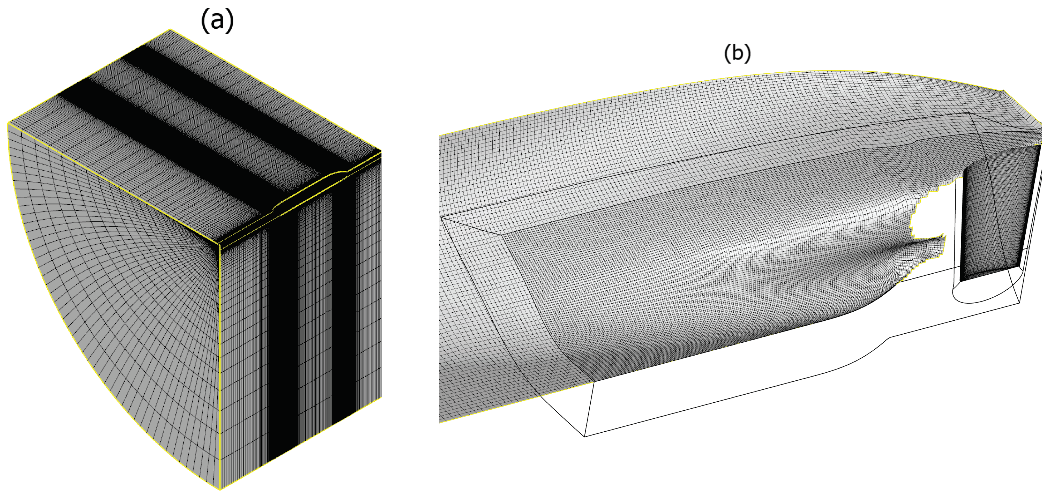
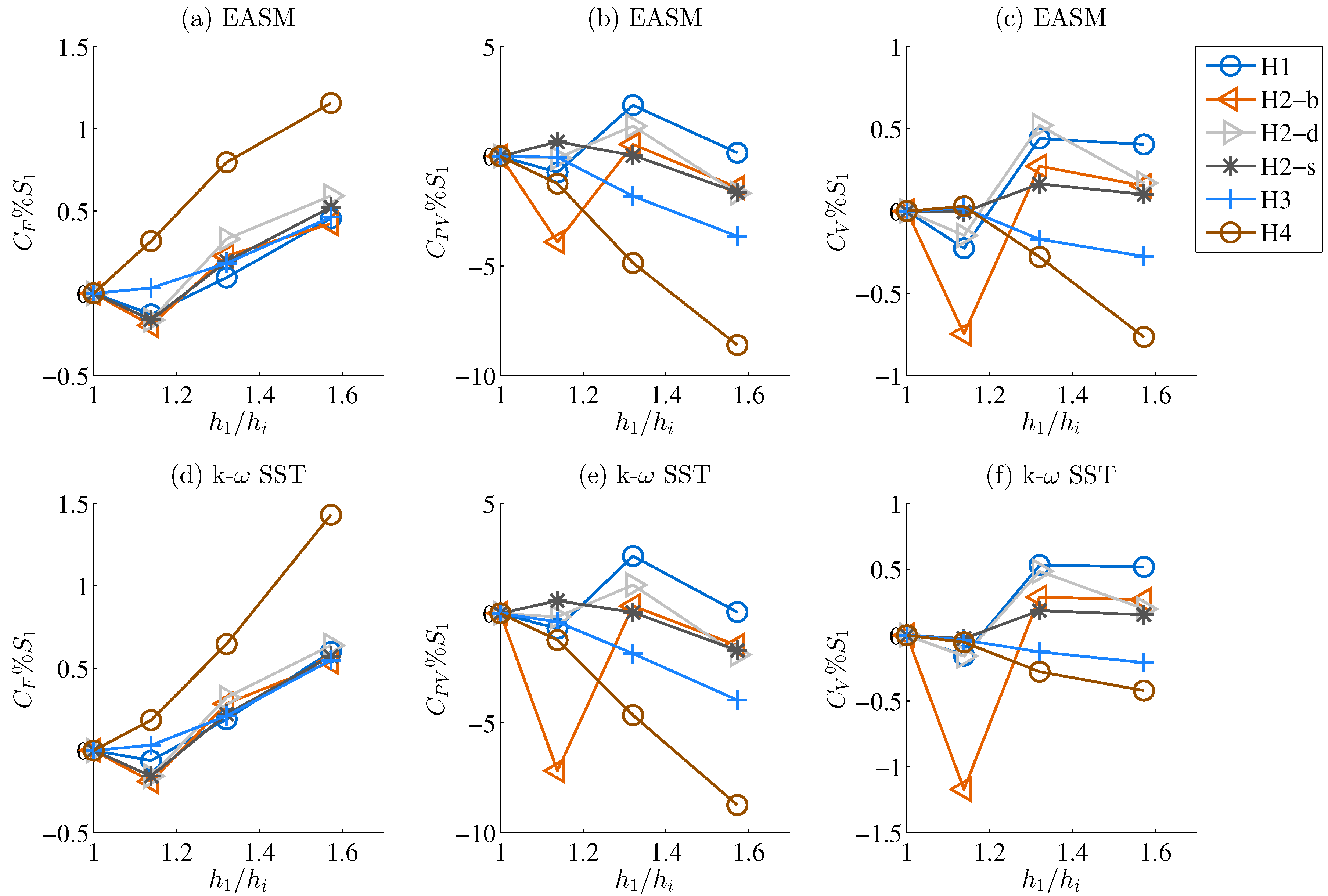
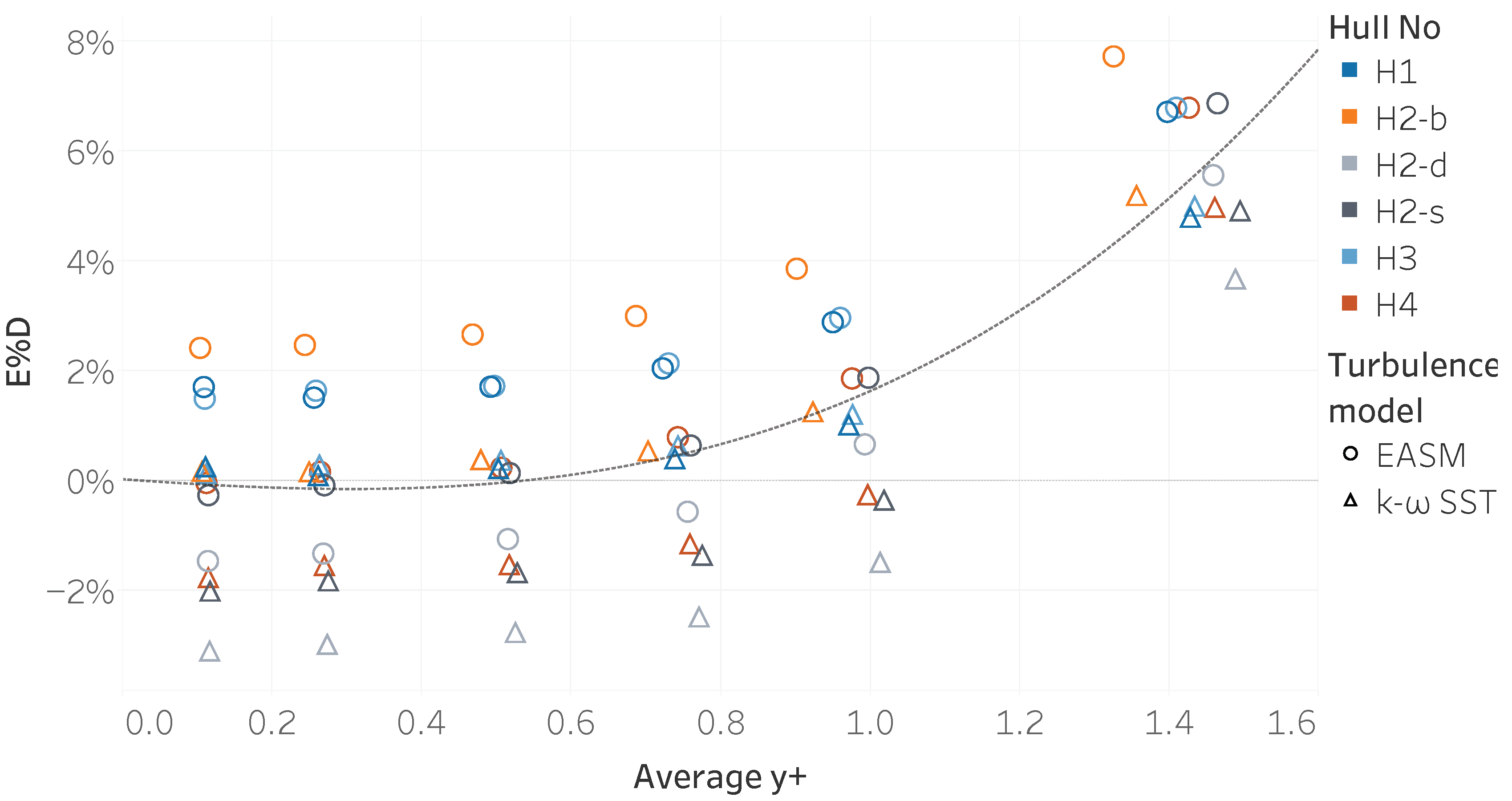
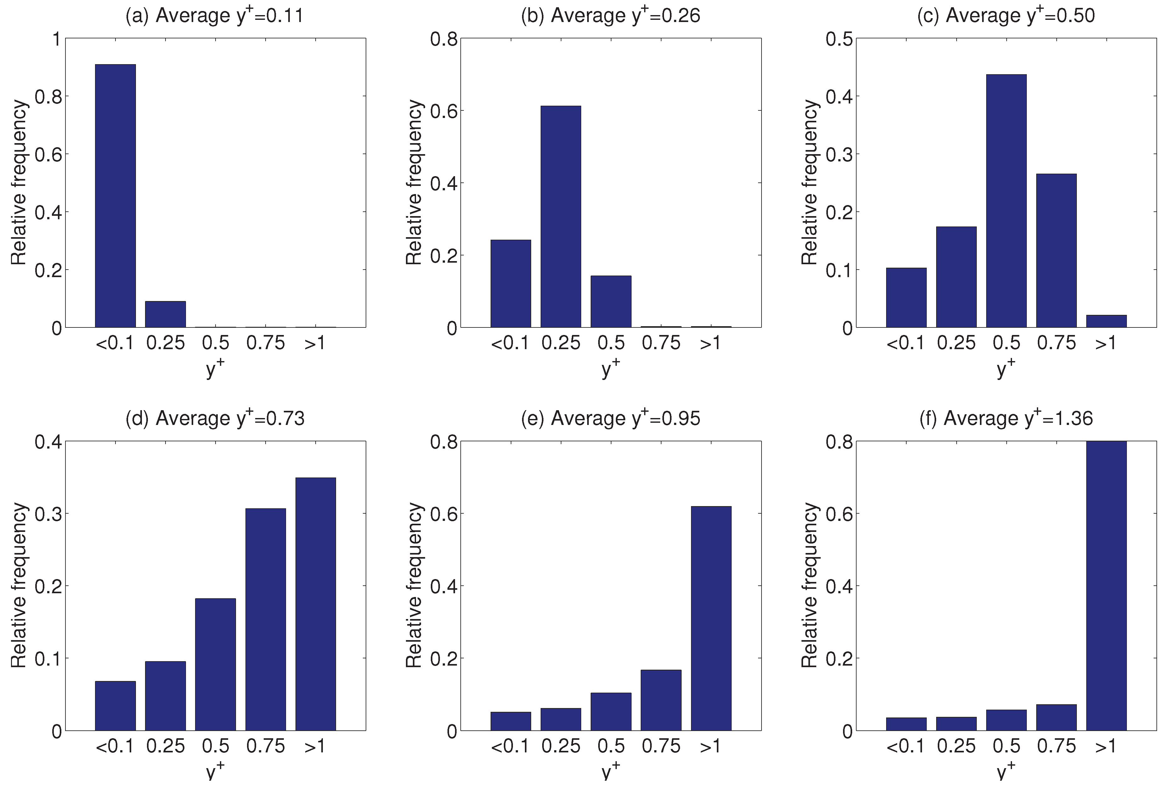
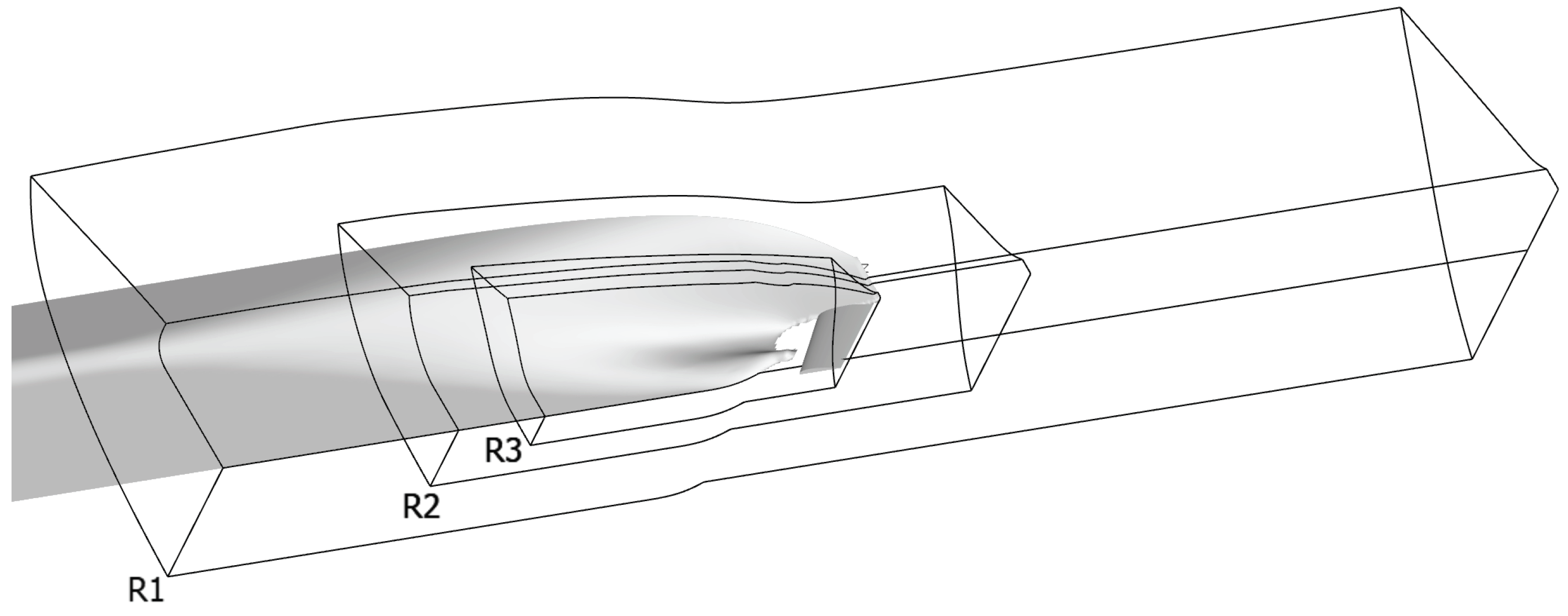
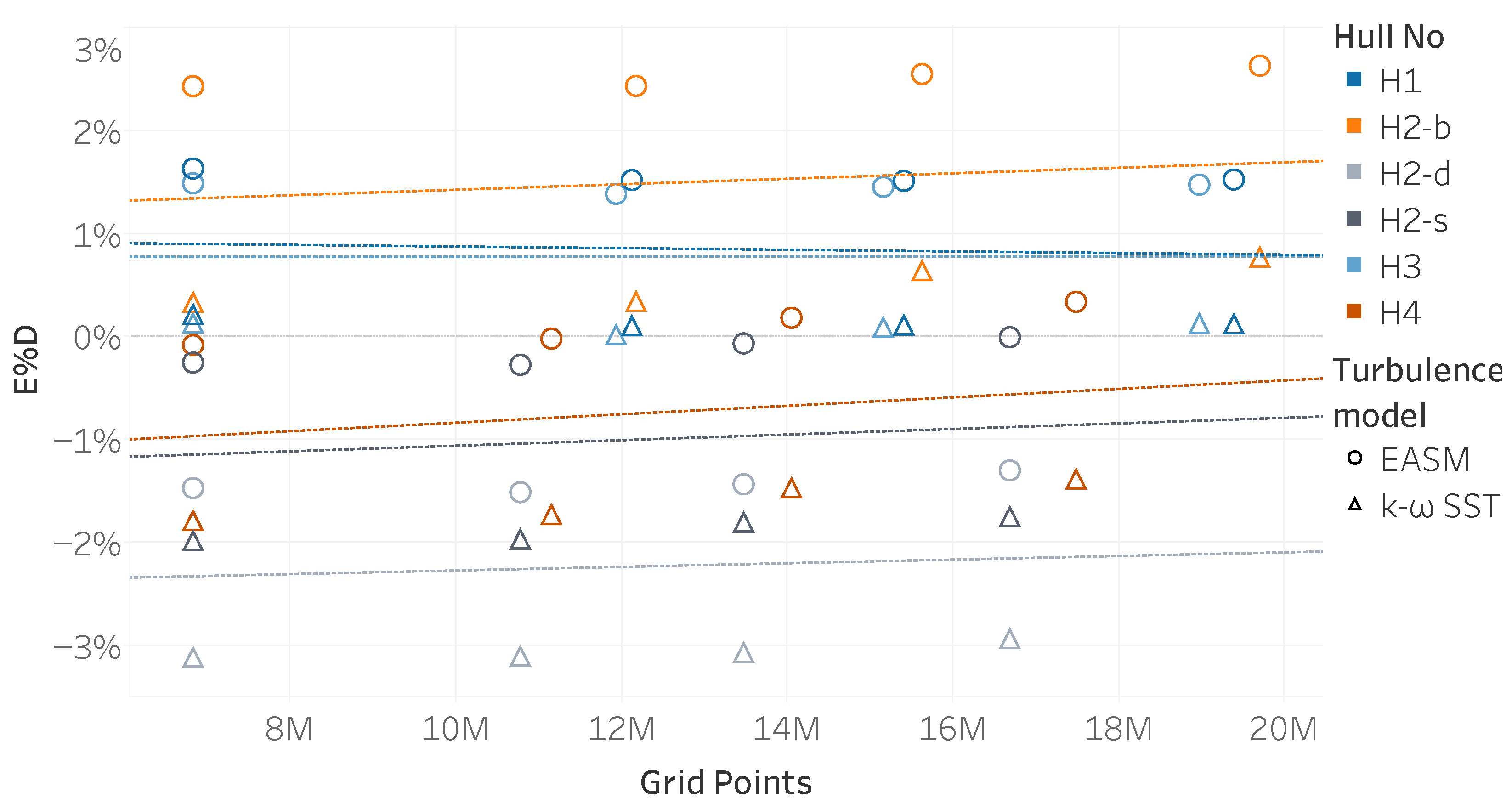
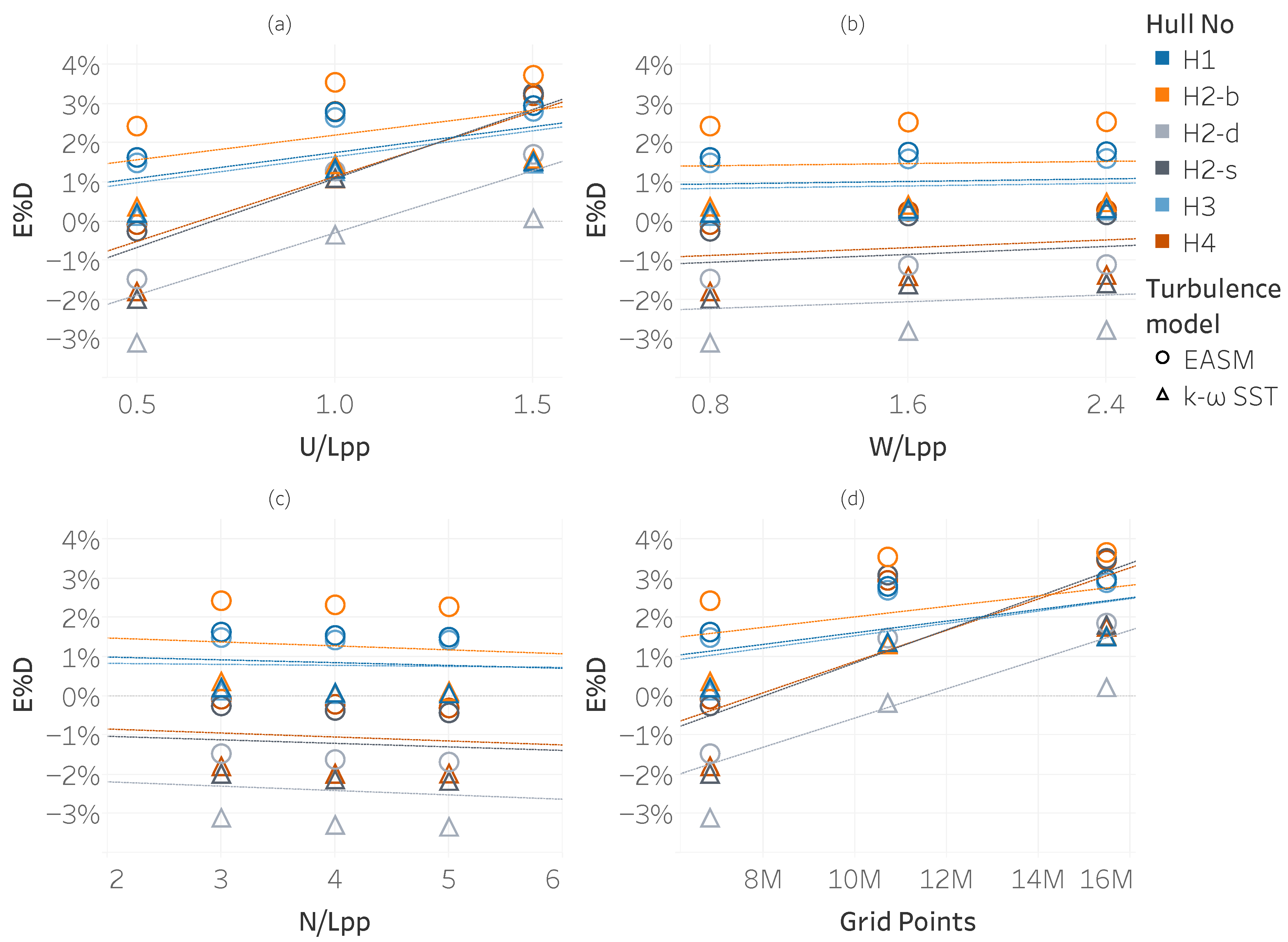
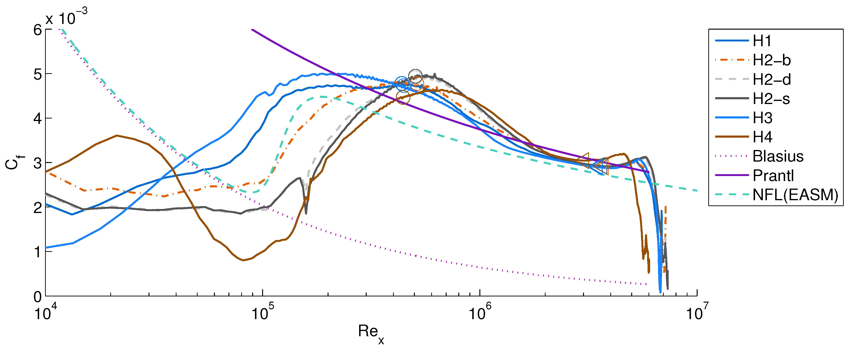
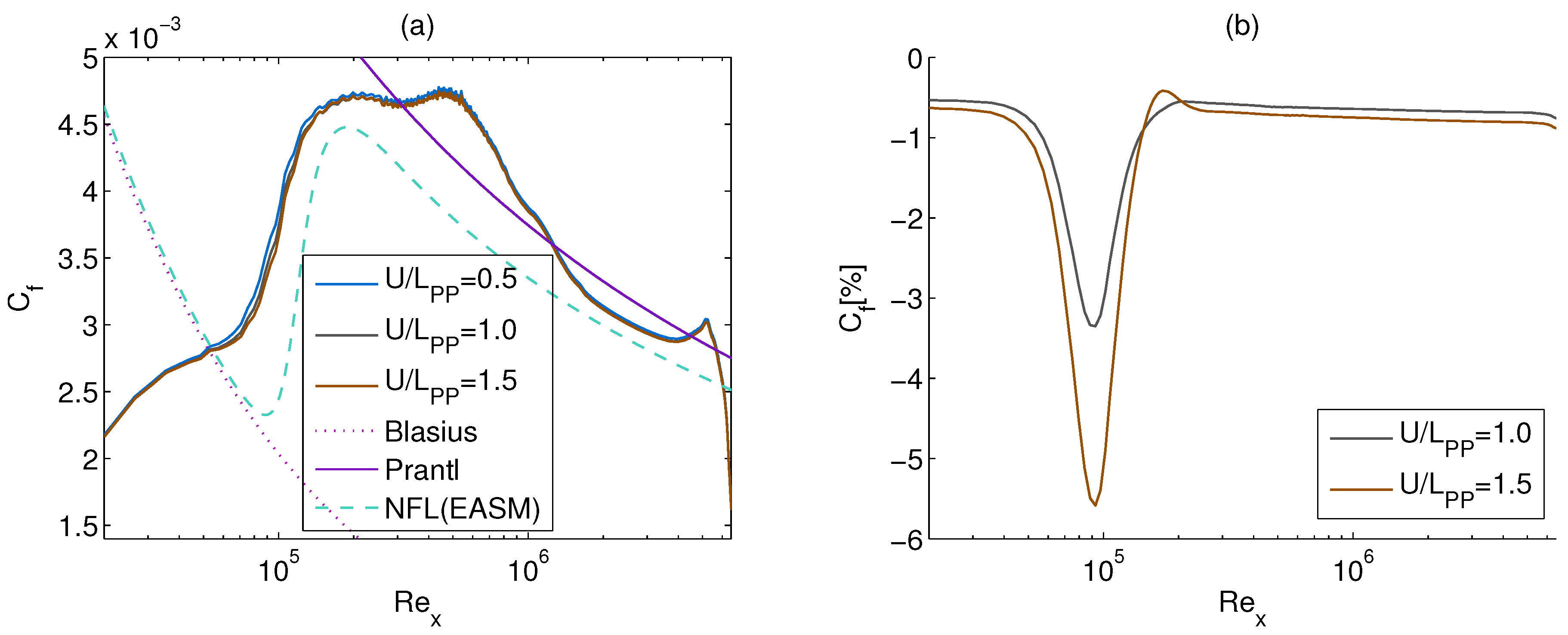
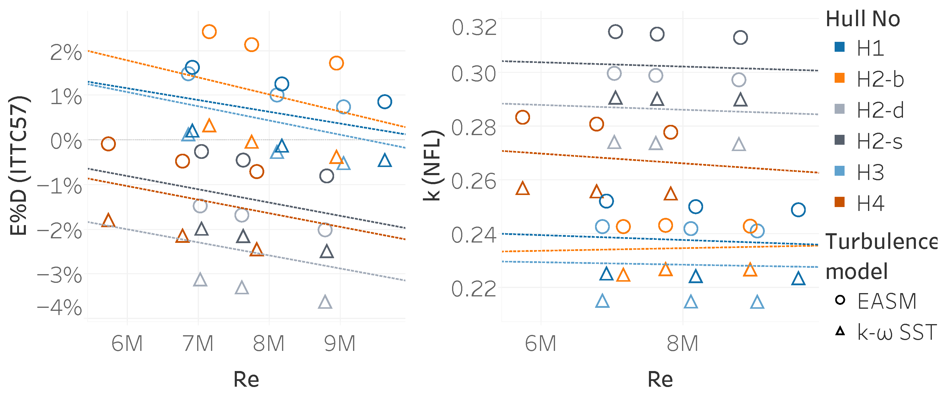
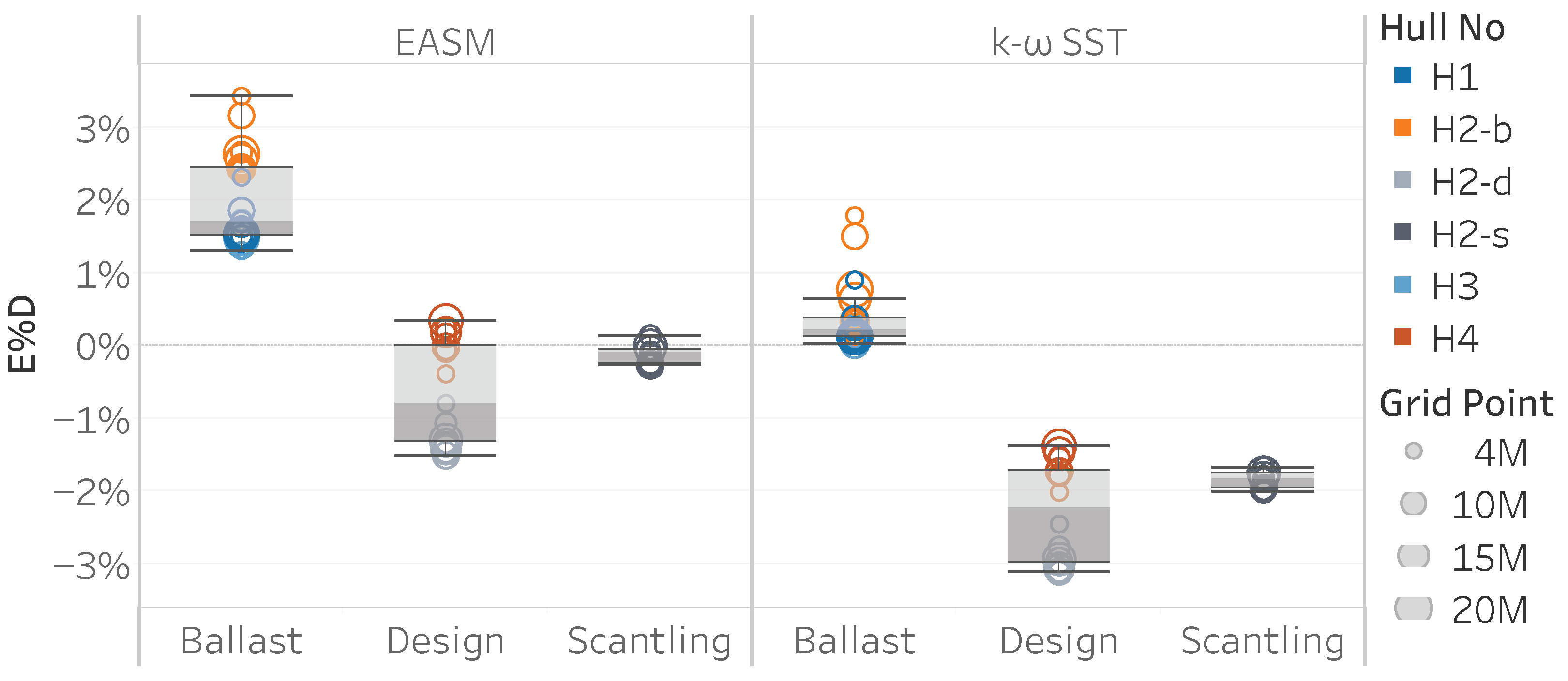
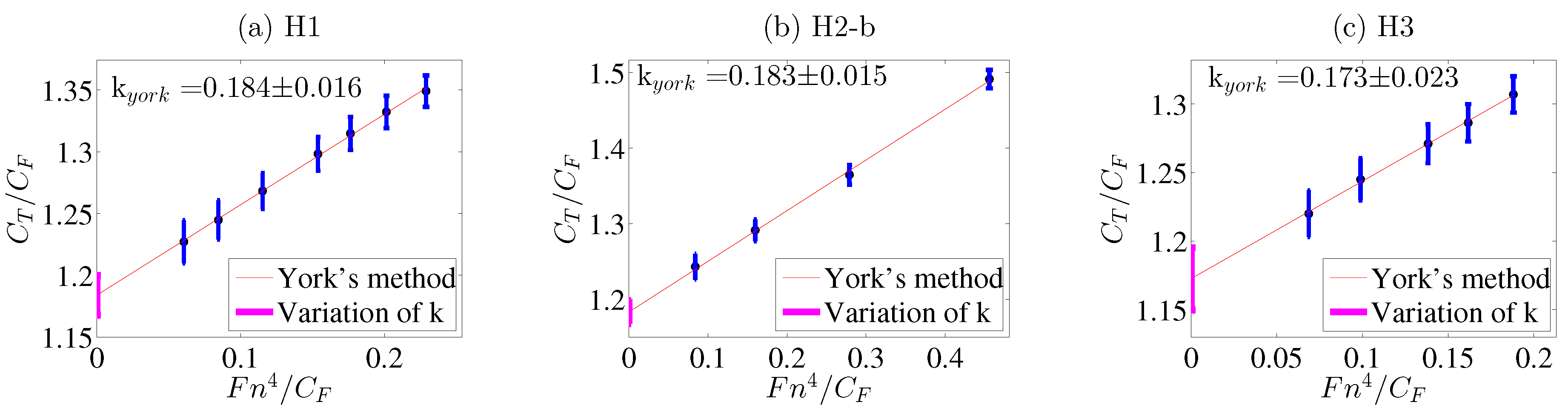
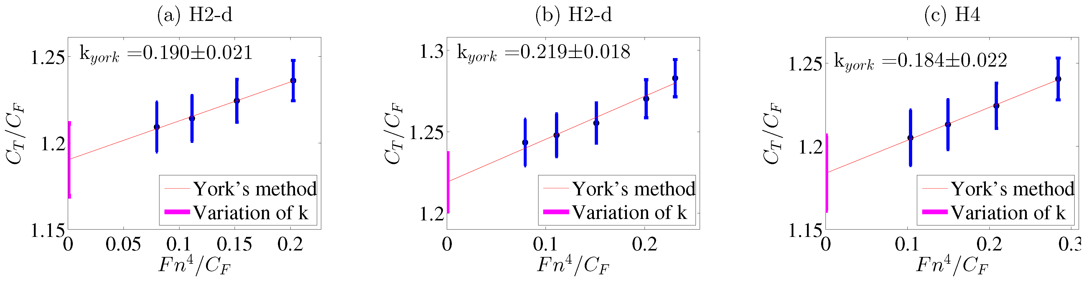
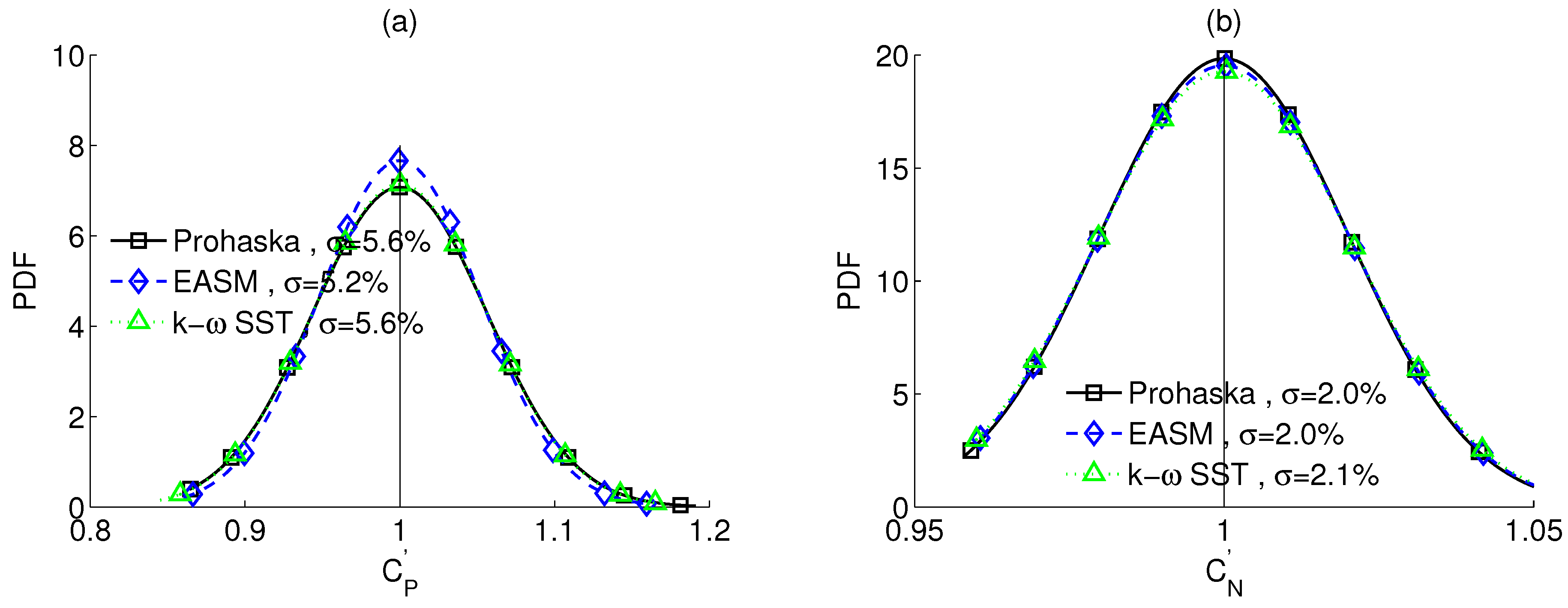
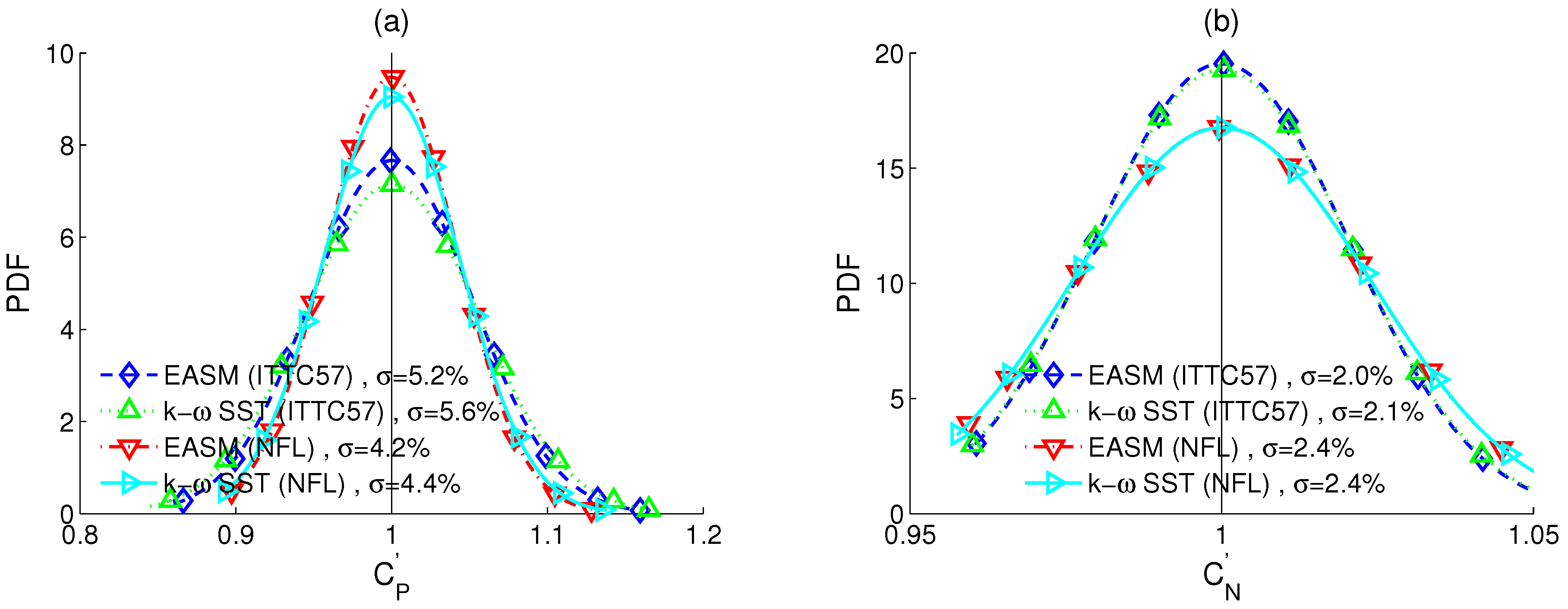
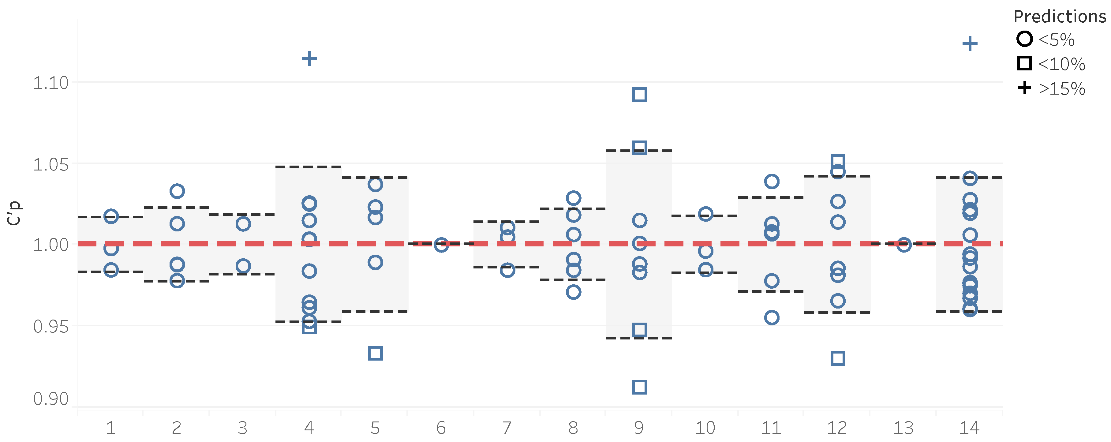
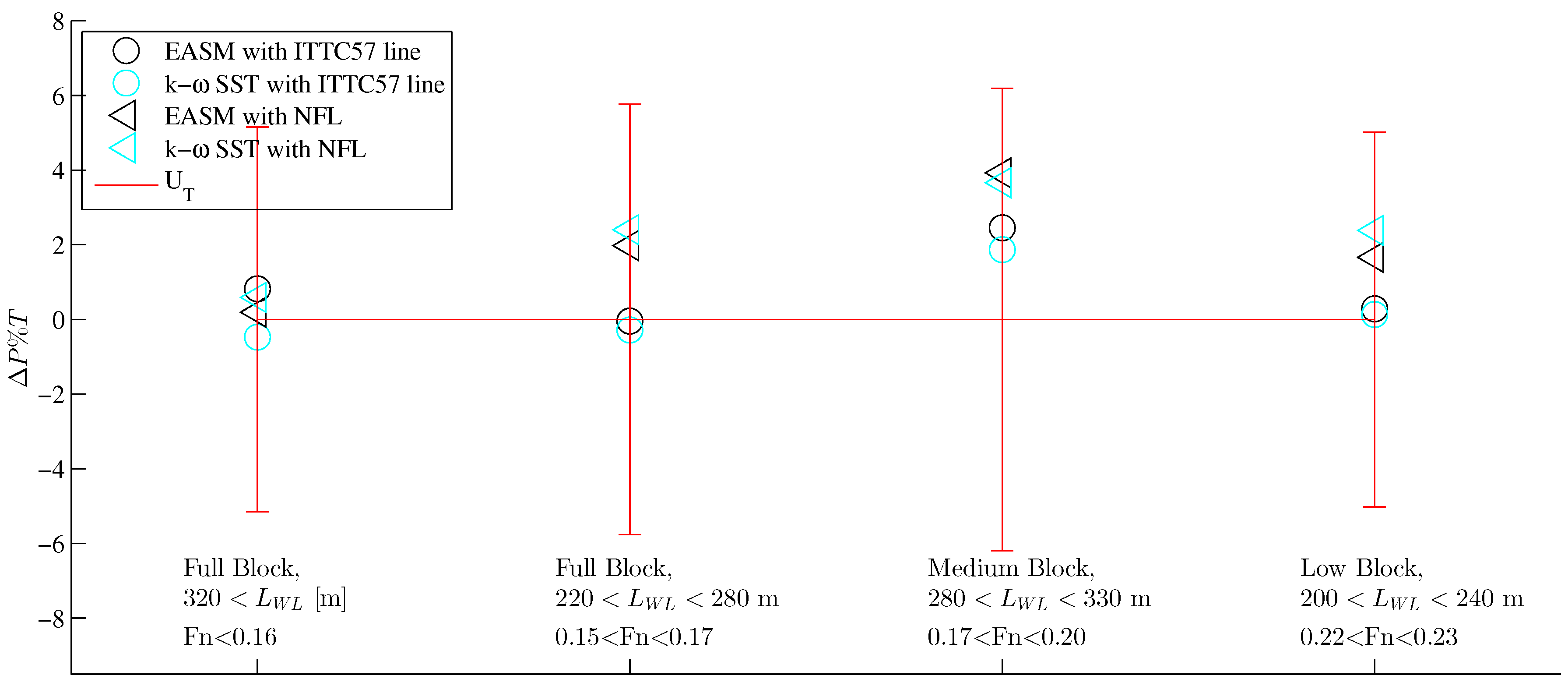
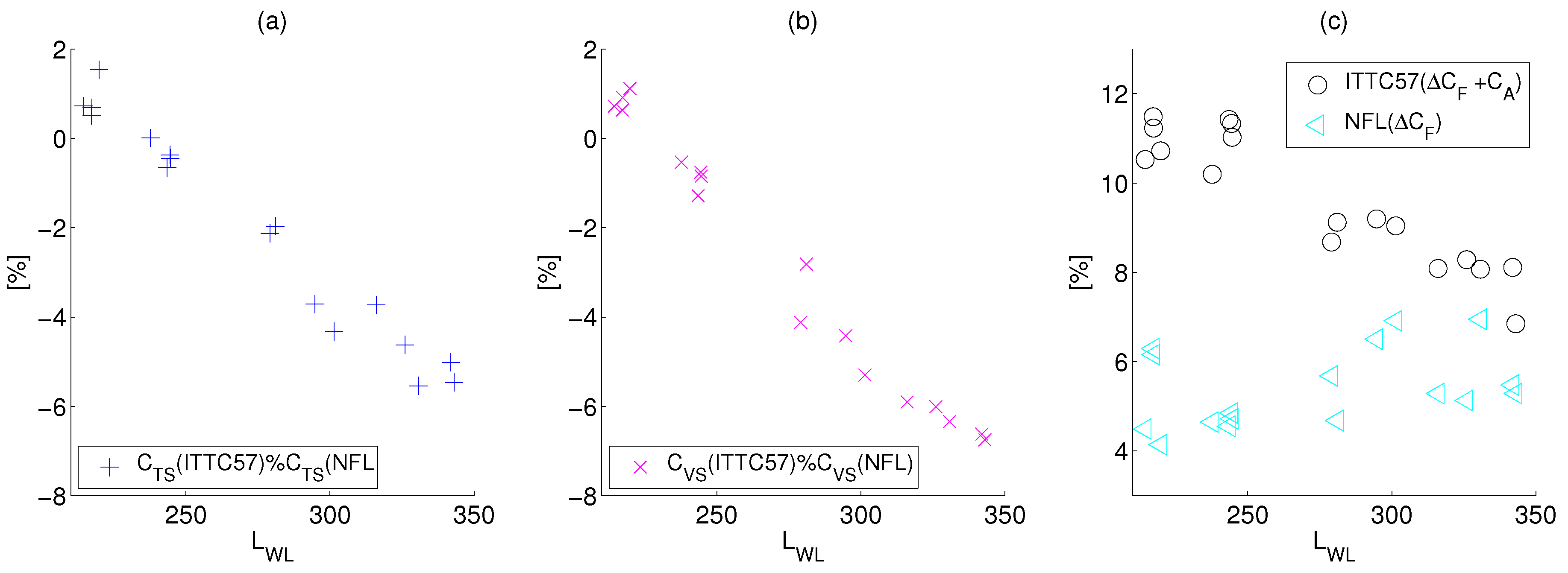
Table 1.
Estimated numerical uncertainties of SHIPFLOW in model scale for EASM and SST turbulence models, in a percentage of the computed result of the finest grid, S.
Table 1.
Estimated numerical uncertainties of SHIPFLOW in model scale for EASM and SST turbulence models, in a percentage of the computed result of the finest grid, S.
| U S | Turb. Model | H1 | H2-b | H2-d | H2-s | H3 | H4 |
|---|---|---|---|---|---|---|---|
| C | EASM | 1.2 | 0.6 | 1.3 | 1.1 | 1.1 | 4.5 |
| SST | 1.5 | 0.7 | 0.5 | 1.2 | 1.3 | 1.0 | |
| C | EASM | 37.2 | 4.1 | 52.6 | 20.1 | 7.8 | 13.2 |
| SST | 61.2 | 4.1 | 52.9 | 20.7 | 9.1 | 8.2 | |
| C | EASM | 6.9 | 1.1 | 10.6 | 4.7 | 2.2 | 6.0 |
| SST | 10.2 | 1.1 | 9.5 | 4.8 | 2.5 | 2.2 |
Table 2.
Validation of the CFD based form factors.
| Form Factor | Turb. Model | H1 | H2-b | H2-d | H2-s | H3 | H4 |
|---|---|---|---|---|---|---|---|
| U D | EASM | 7.6 | 2.0 | 11.7 | 5.4 | 2.9 | 7.0 |
| SST | 11.2 | 2.5 | 10.7 | 5.6 | 3.2 | 3.2 | |
| U D | - | 1.3 | 1.3 | 1.8 | 1.5 | 2.0 | 1.8 |
| D | EASM | 1.6 | 2.4 | 1.1 | 0.3 | 1.5 | 0.1 |
| SST | 0.2 | 0.3 | 2.8 | 2.0 | 0.1 | 1.8 | |
| U D | EASM | 7.7 | 2.4 | 11.9 | 5.7 | 3.5 | 7.2 |
| SST | 11.2 | 2.8 | 10.8 | 5.8 | 3.8 | 3.7 |
Table 3.
Statistics of the power predictions compared to speed trial.
| u< | Number Speed Trials | Quantitiy | Standard ITTC-78 | CFD Based k, ITTC-57 Line with EASM | CFD Based k, ITTC-57 Line with SST | CFD Based k, NFL with EASM | CFD Based k, NFL with SST |
|---|---|---|---|---|---|---|---|
| 4.9% | 4.7% | 5.0% | 4.3% | 4.3% | |||
| 4 | 46 | 5% < Error <10% | 19% | 15% | 19% | 13% | 13% |
| 10% < Error | 7% | 9% | 9% | 4% | 4% | ||
| 5.8% | 5.3% | 5.7% | 4.4% | 4.6% | |||
| 6 | 69 | 5% < Error <10% | 21% | 19% | 24% | 18% | 19% |
| 10% < Error | 9% | 9% | 9% | 4% | 4% | ||
| 5.6% | 5.2% | 5.6% | 4.2% | 4.4% | |||
| 8 | 78 | 5% < Error <10% | 20% | 20% | 24% | 11% | 16% |
| 10% < Error | 9% | 8% | 9% | 4% | 5% |
Publisher’s Note: MDPI stays neutral with regard to jurisdictional claims in published maps and institutional affiliations. |
© 2021 by the authors. Licensee MDPI, Basel, Switzerland. This article is an open access article distributed under the terms and conditions of the Creative Commons Attribution (CC BY) license (http://creativecommons.org/licenses/by/4.0/).
Share and Cite
MDPI and ACS Style
Korkmaz, K.B.; Werner, S.; Bensow, R. Verification and Validation of CFD Based Form Factors as a Combined CFD/EFD Method. J. Mar. Sci. Eng. 2021, 9, 75. https://doi.org/10.3390/jmse9010075
AMA Style
Korkmaz KB, Werner S, Bensow R. Verification and Validation of CFD Based Form Factors as a Combined CFD/EFD Method. Journal of Marine Science and Engineering. 2021; 9(1):75. https://doi.org/10.3390/jmse9010075
Chicago/Turabian StyleKorkmaz, Kadir Burak, Sofia Werner, and Rickard Bensow. 2021. "Verification and Validation of CFD Based Form Factors as a Combined CFD/EFD Method" Journal of Marine Science and Engineering 9, no. 1: 75. https://doi.org/10.3390/jmse9010075
Note that from the first issue of 2016, this journal uses article numbers instead of page numbers. See further details here.