PM_2.5 Estimation and Spatial-Temporal Pattern Analysis Based on the Modified Support Vector Regression Model and the 1 km Resolution MAIAC AOD in Hubei, China

Abstract

The satellite-retrieved Aerosol Optical Depth (AOD) is widely used to estimate the concentrations and analyze the spatiotemporal pattern of Particulate Matter that is less than or equal to 2.5 microns (PM_2.5), also providing a way for the related research of air pollution. Many studies generated PM_2.5 concentration networks with resolutions of 3 km or 10 km. However, the relatively coarse resolution of the satellite AOD products make it difficult to determine the fine-scale characteristics of PM_2.5 distributions that are important for urban air quality analysis. In addition, the composition and chemical properties of PM_2.5 are relatively complex and might be affected by many factors, such as meteorological and land cover type factors. In this paper, an AOD product with a 1 km spatial resolution derived from the Multi-Angle Implementation of Atmospheric Correction (MAIAC) algorithm, the PM_2.5 measurements from ground sites and the meteorological data as the auxiliary variable, are integrated into the Modified Support Vector Regression (MSVR) model that proposed in this paper to estimate the PM_2.5 concentrations and analyze the spatiotemporal pattern of PM_2.5. Considering the relatively small dataset and the somewhat complex relationship between the variables, we propose a Modified Support Vector Regression (MSVR) model that based on SVR to fit and estimate the PM_2.5 concentrations in Hubei province of China. In this paper, we obtained Cross Correlation Coefficient (R²) of 0.74 for the regression of independent and dependent variables, and the conventional SVR model obtained R² of 0.60 as comparison. We think our MSVR model obtained relatively good performance in spite of many complex factors that might impact the accuracy. We then utilized the optimal MSVR model to perform the PM_2.5 estimating, analyze their spatiotemporal patterns, and try to explain the possible reasons for these patterns. The results showed that the PM_2.5 estimations retrieved from 1 km MAIAC AOD could reflect more detailed spatial distribution characteristics of PM_2.5 and have higher accuracy than that from 3 km MODIS AOD. Therefore, the proposed MSVR model can be a better method for PM_2.5 estimating, especially when the dataset is relatively small.

1. Introduction

Currently, air pollution and its related health problems have become research hot spots [1]. Numerous studies have indicated that particles smaller than 2.5$\mathsf{\mu }\mathrm{m}$ in aerodynamic diameter (PM_2.5) have adverse effects on human health and can cause pulmonary and cardiovascular diseases [2,3].

People exposed to polluted environments are prone to illness or even death. Thus, PM_2.5 exposure monitoring and pattern analysis are critical to air quality assessment and environmental epidemiologic studies [4,5]. PM_2.5 concentrations are traditionally obtained by ground monitoring sites distributed throughout a country. However, the existing ground monitoring sites are too sparse to provide continuous PM_2.5 monitoring due to the high construction cost. In contrast, satellite remote sensing has wide and continuous spatial coverage and has been widely applied in the estimation of PM_2.5 concentrations [6,7], although the cloud could affect the availability of data.

Satellite-derived Aerosol Optical Depth (AOD) represents the quantity of light removed from a beam by the role of aerosol scattering or absorption during its path [8,9]. Furthermore, previous studies have indicated that there exists a direct relationship between the atmospheric particles (such as PM_2.5) and AOD [10]. Thus, remote sensing satellites’ AOD products provide a potentially cost-effective way to estimate ground-level PM_2.5 mass concentrations [11,12]. A series of AOD products have been applied to such surveys [13], e.g., the Moderate Resolution Imaging Spectroradiometer (MODIS) [14,15], the Multi-angle Imaging Spectroradiometer [16], the Himawari-8 (H8) [17,18], and the Visible Infrared Imaging Radiometer Suite [19]. However, the relatively coarse spatial resolutions (usually 3 km or 10 km) of the above-mentioned satellite sensors limit the precise estimates of PM_2.5 in urban areas. Recently, the Multi-Angle Implementation of Atmospheric Correction (MAIAC) algorithm, which utilizes time-series analysis and image-based processing techniques, was developed to conduct aerosol retrievals and atmospheric corrections.

The Multiangle Implementation of Atmospheric Correction (MAIAC) is a new generic algorithm applied to collection 6 (C6) MODIS measurements to retrieve Aerosol Optical Depth (AOD) over land at high spatial resolution (1 km) [20]. The related AOD product MCD19A2 (MODIS Collection 6 (C6) daily AOD dataset), which is based on the MAIAC algorithm, was released in 2018 [21]. Although the goal of the MAIAC AOD product is aerosol monitoring, this product of 1 km resolution gives us chance to estimate PM_2.5 concentrations in a higher spatial and temporal resolution.

Previous studies have shown that the relationship between PM_2.5 and AOD is relatively complex and may be affected by a series of parameters, such as the aerosol type and the vertical structure of aerosol distribution [22], the relative humidity (RH) [23], planetary boundary layer height (PBLH) [24], wind speed and direction [25], the depth and temperature difference of the inversion layer [24], land cover [26], etc. Furthermore, recently, more sophisticated methods used to estimate PM_2.5 have been developed by taking into account these parameters.

Studies have tried to explore the relationship between these variables by statistical approaches. There have been many different approaches proposed by studies that explored the relationship between PM_2.5 and AOD. For example, including but not limited to, the linear regression model, the geographically weighted regression model [27,28], the two-stage model [29] and the newly developed neural network methods [30,31]. As geospatial data, PM_2.5 concentration data have spatial heterogeneity and spatial dependence. The statistical characteristics of PM_2.5 concentrations may vary over space and time. This space–time anisotropy may violate the independent and identically distributed random variables in most of the machine learning methods [32].

The Support Vector Machine (SVM) based on the principle of structural risk minimization initially developed for solving classification problems using small sample learning is found to be promising for solving regression problems. The SVM for regression termed as Support Vector Regression (SVR) has revealed superior performance due to its inherent capability to circumvent overfitting problem in regression and improved response approximation ability [33].

Considering the characteristics of the experiment:

1. Nonlinear and complex relationship; as an atmospheric research, the relationship between PM_2.5, AOD and auxiliary variables is rather complicated and it would be better to describe it with nonlinear model. The kernel function can simplify the inner product operation in the mapping space, avoiding calculating in the high-dimensional space directly.

2. The relatively small dataset. Regression algorithms generally obey the law of big data; this means that the final result is relatively more accurate with more samples. The SVM makes it possible to achieve relatively good results on small samples. SVR based on the support vector machine solves regression problems using small sample learning. Furthermore, the ′small sample′ is a considerable concept; we think the samples in our experiment are enough for digging out the nonlinear relationship.

3. The capability to handle high-dimensional data sets well. SVR can grasp the nonlinear relationship between data and features on relatively small datasets, especially compared to most other machine learning methods.

Thus, this paper proposes the modified SVR (MSVR) method to improve the estimation accuracy of PM_2.5 concentrations. MSVR considers the impacts of spatial distance on estimation accuracy and adds factors in the model input that are generally included and contribute relatively more significant influence, with MAIAC AOD as the primary predictor and the meteorological and land cover information as ancillary information.

2. Materials and Methodology

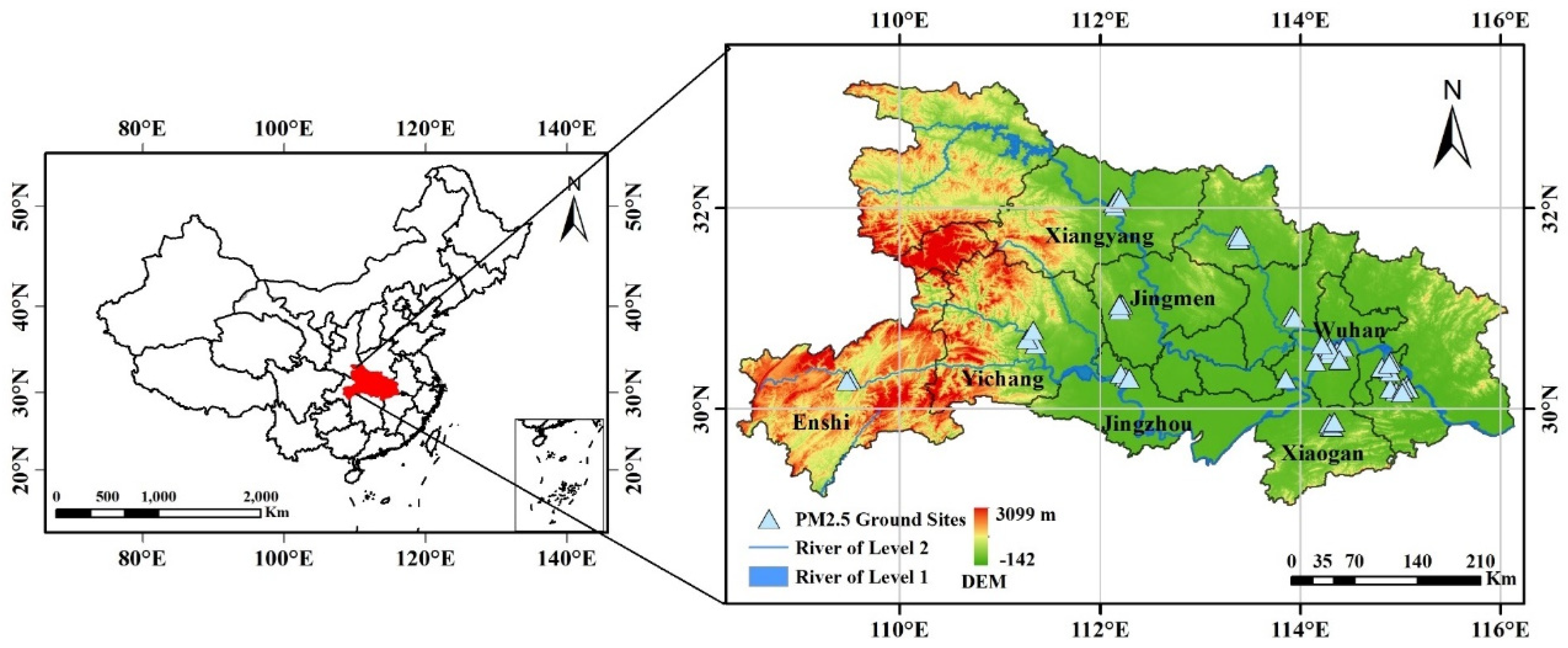
2.1. Study Area

The study area of this paper is Hubei, China. Hubei Province is located in central China, and its capital city, Wuhan, is one of the largest cities and developing centers of the country (Figure 1). With the rapid development of urbanization and industrialization in China, climate disasters, such as smog, frequently occur in large cities in China as a result of worsening atmospheric and environmental conditions [34]. Research on PM_2.5 estimation and analysis in Wuhan can provide constructive guidance for urban air quality research in other large cities in China. Meanwhile, due to the complex climate and land cover of Hubei Province, research in this area can help analyze the effects of various factors such as climate and land cover on PM_2.5 distribution.

2.2. Experimental Data

2.2.1. MAIAC and MODIS AOD Data

The MAIAC algorithm is an advanced algorithm for aerosol retrievals and atmospheric correction for MODIS data over both dark vegetated and bright desert surfaces. This algorithm explores the advantages of time-series processing at a synergistic level for cloud masking and aerosol-surface retrievals. The MAIAC algorithm uses up to 16 days of gridded MODIS measurements to make simultaneous retrievals of AOD and surface bidirectional reflectance distribution factor (BRF)/albedo and then produces the AOD at a 1 km resolution. The algorithm uses both individual grid cells (also called pixels) and fixed-size (25 × 25 km²) areas (also called blocks), as required by the cloud mask algorithm and retrieval [21].

Studies have indicated that MAIAC AOD agreed well with AERONET AOD (Aerosol Robotic Network AOD), which is commonly considered as the ground true values of AOD [35]. Additionally, comparison studies between the satellite AOD and the AERONET AOD showed that the MAIAC algorithm improved the accuracy than MODIS DB (Deep Blue)/DT (Dark Target) [36]. Mhawish [20] obtained RMSE 0.148 for MAIAC, 0.198 for MODIS DB, and 0.183 for MODIS DT.

AERONET AOD currently has 61 stations distributed in China, but there are no stations in our research area, Hubei Province. Therefore, we may not be able to conduct a comparison of AERONET and MODIS data in the study area of the study period. Furthermore, there has been research that gained the insights regarding the performance of MAIAC algorithm by comparing MAIAC aerosol products with the ground-based observations at nine typical sites spread out in China. The research indicated that MAIAC and ground-observed AOD values showed high correlation coefficient (R of most sites reached higher than 0.85 or even 0.9) in spite of the complicated surface types, diverse aerosol sources, and heavy loading of aerosols in the vast atmosphere of China. MODIS MAIAC 1 km AOD at 550 nm, compared with AERONET measurements in Xuzhou and Taihu sites that are relatively close to our research area, obtained R of 0.91 and 0.878. More and more studies have applied MAIAC AOD to PM_2.5 inversion in China. We believe that this AOD product has quality assurance over China.

2.2.2. Auxiliary Variables

Because atmospheric flow is affected by meteorological parameters (e.g., temperature and humidity) [25] and because air pollutants may be absorbed by some land cover types (e.g., vegetation) [37], meteorological parameters and land cover parameters were adopted as auxiliary variables in our algorithm to improve the estimation accuracy of PM_2.5.

• Meteorological data

Boundary layer height (BLH, m) refers to the thickness of the planet’s boundary layer and is one of the important physical parameters for atmospheric numerical model and atmospheric environment evaluation. Usually, BLH has a negative relationship with PM_2.5 because a higher BLH can expand the near-surface atmosphere and facilitate vertical convection. Humidity can influence the concentration of PM_2.5 by changing the weight of particulates and further affecting the diffusion speed of pollutants [38]. Temperature has a negative relationship with PM_2.5 because the inversion layer caused by low temperature is not conducive to the convection of the atmosphere [39]. Therefore, in this paper, the three types of meteorological parameters, BLH, relative humidity (RH, %), and 2 m near-ground-temperature (T, °C), were adopted in our algorithm to improve the estimation accuracy.

The BLH, RH, and T data employed in this paper were obtained from the European Centre for Medium-Range Weather Forecasts (ECMWF) (https://www.ecmwf.int/). The ECMWF provides quality controlled spatially and temporally consistent, real-time, current forecasts, climate reanalysis and specific datasets. The data assimilation system used to produce ERA-Interim was based on a 2006 release of the IFS (Cy31r2). The system includes a 4-dimensional variation analysis (4D-Var) with a 12-h analysis window. The spatial resolution of the data set is approximately 80 km (T255 spectral) on 60 vertical levels, from the surface up to 0.1 hPa, and at a horizontal resolution of 0.125° × 0.125º, and its temporal resolution is 3 h.

• Land cover data

Land cover variables, especially vegetation coverage and construction parameters, can influence the performance of the AOD-PM_2.5 regression models [40]. Studies have shown that vegetation coverage has an obvious effect on reducing and redistributing atmospheric particulate matters by means of sedimentation, retardation and adsorptions. It is worth noting that these effects will change with the change of seasons, because some vegetation will have different states in different seasons. Generally, winter vegetation has the smallest reduction effect on PM_2.5 [41]. Conversely, construction land produces dust and other pollutants that increase the concentration of atmospheric pollutants.

Land cover data with a 1 km spatial resolution were utilized in this paper. The data were obtained from the “Remote sensing monitoring data of land cover in China” section on the website of the Chinese Academy of Sciences Data Centre for Resources and Environmental Sciences (http://www.resdc.cn). It provides a database of multi-phase land cover status for the national land area under the years of accumulation generated by manual visual interpretation and based on the Landsat TM/ETM remote sensing image data. The land cover types include six primary types: cultivated land, forestland, grassland, waters, residential areas and unused land.

2.2.3. Ground PM_2.5 Measurements

The ground PM_2.5 measurements were used as training data and testing data in our algorithm to obtain the relationship between PM_2.5 and AOD and were then utilized to generate continuous PM_2.5. As shown in Figure 1, there are 47 national ground monitoring sites in the study area (Hubei Province). The 47 sites are mainly located in densely populated cities, such as Wuhan (10 sites), and there are rural areas without ground sites. The PM_2.5 measurements in four seasons of 2017 from these sites were used in the experiment of this paper. The PM_2.5 hourly data were collected from the PM25.IN website (http://www.pm25.in/) provided by the China National Environmental Monitoring Center (CNEMC); as for worldwide research, the PM_2.5 data can be obtained from the following website (http://www.aqicn.info/here/).

Terra and Aqua satellites passed over the equator at approximately 10:30 a.m. and 13:30 p.m. local time [42]. To ensure the time consistency of AOD and PM_2.5, we took the average of the hourly PM_2.5 measurements from 10:00 AM to 14:00 PM.

2.2.4. Data Pre-Processing and Integration

All the data and the descriptions were listed in

Table 1. List of the data and variables adopted in the experiment.

Variables	Unit	Description	Temporal Period
PM2.5	μg/m3	Particulate matter smaller than 2.5 $\mathsf{\mu }\mathrm{m}$ in aerodynamic diameter	Hourly average of 10:00 am to 13:00 pm
AOD		Satellite-retrieved Aerosol Optical Depth	Daily data
RH	%	Relative Humidity	Hourly instantaneous data
BLH	(m)	Boundary Layer Height
T	°C	2 m Temperature
Land Cover		Vegetation coverage and construction factors	Remote sensing monitoring data of China’s land use status in 2015

.

Four types of data were used in MSVR, including AOD, meteorological factors, land cover, and ground PM_2.5, and data pre-processing and integration were required due to the differences in the spatial coverage and observation frequency of the data. To ensure the spatial consistency of the data from multiple sources, all data were first re-projected to a unified coordinate system: The World Geodetic System 1984 geographic coordinate system [43,44].

On the one hand, the atmosphere is moving and circulating, thus the concentration of atmospheric particles at a certain location changes over time. On the other hand, variables in this research are not instantaneous data, but the average over a certain period of time. Therefore, we took the weighted average of 3 × 3 pixels centered on the grid.

Meanwhile, the forest and construction land-use data that significantly affected the formation and concentration of PM_2.5 were extracted with a buffer of 1 km from the ground monitoring sites. In terms of temporal consistency, the meteorological data were integrated to the average of the period from 10:00 AM to 14:00 PM local time to correspond to the period when Terra and Aqua passed over the equator. The extraction and integration of multi-source data were mainly implemented by coding in Python.

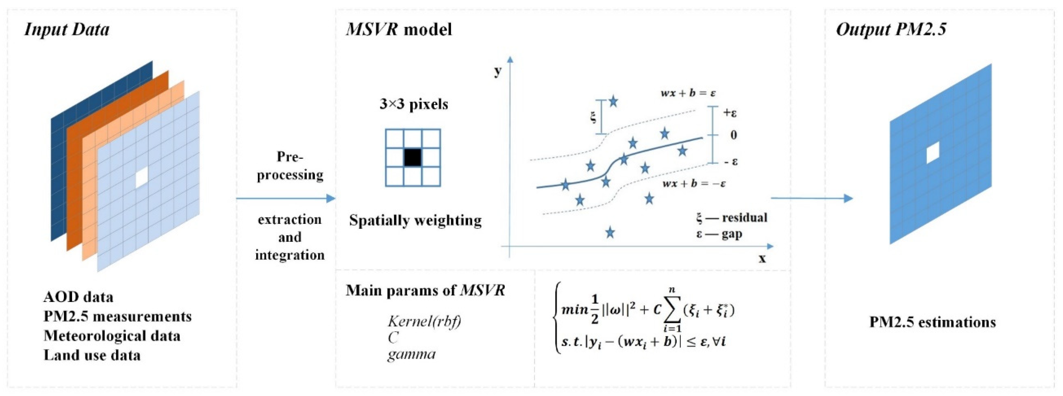
2.2.5. Model Constructing and Training

For better performance of MSVR, the datasets including all variables were first normalized to [0, 1]. As for the parameter setting of the MSVR model, we selected the RBF kernel for the kernel function considering the complicated relationships between all the variables. We listed a series of value combinations of the parameters “gamma” and “C” (penalty parameter) and then chose the optimal parameter values by grid searching.

Five-fold cross validation was employed in this experiment. The training dataset was first randomly split into five subsets, with approximately 20% of the total data record in each subset. In each round of cross-validation, one subset was selected to be used as validation samples, and the remaining subsets were utilized to train and fit the model.

In this experiment, three statistical indicators, including the R², the mean percentage error (MPE) and the square root of the mean squared prediction errors (RMSE), were calculated to assess the model performance. The accuracy evaluation and the comparison of the different models are discussed later in Section 4.1.

2.3. Principle of SVR

A Support Vector Machine (SVM) is a kind of machine learning method based on statistical learning theory, dimension theory and structural risk minimization principle. It shows many unique advantages in solving small sample, nonlinear and high-dimensional pattern recognition problems, and to a large extent overcomes the problems of “dimension disaster” and “over-learning” [45]. SVM is widely used to solve problems such as classification and nonlinear mapping and performs better in solving the problem of small sample datasets. SVM can, to a certain extent, solve the problems of model selection and over-learning that may be difficult for some traditional networks to solve.

Support Vector Regression (SVR) is the application of SVM in regression analysis [46], and it solves the regression task by transforming an inseparable problem of low-dimensional space into a linearly separable problem of high-dimensional space using the space mapping function [47]. We must find a hyperplane to fit the distribution of the sample data, which means minimizing the sum of the distance between the sample points and the hyperplane [48,49].

In this experiment, for a given set of training data, the variables $x, y$ are both vectors. $\left\{\left(x_1, y_1\right), \left(x_2, y_2\right), \cdots ,\left(x_i, y_i\right)\right\}, x\subset {\mathbf{R}}^{\mathit{n}} and y\subset \mathbf{R}$, the problem of regression is to find the flattest function $\mathit{f}$ that map a point in the space ${\mathbf{R}}^{\mathit{n}}$ onto the space $\mathbf{R}$ with the lowest expected risk.

The key of nonlinear SVR is to map the input vector $\mathrm{X}\in {\mathbf{R}}^{\mathit{n}}$ into a high dimensional feature space $H\in {\mathrm{R}}^m$ (with m larger than n), through mapping and then to solve a linear regression in space $H$.

$$\phi \left(X\right):X\to H$$

(1)

We call $\phi \left(X\right)$ the mapping function, and usually the mapping function is difficult to calculate. Therefore, the kernel function $K\left(x, y\right)$ is introduced into SVR, where $\langle \varnothing \left(x\right), \varnothing \left(y\right)\rangle$ stands for the scalar product mapped to the feature space.

$$K\left(x, y\right)= \langle \varnothing \left(x\right), \varnothing \left(y\right)\rangle$$

(2)

In the high dimensional space, we can find a hyperplane to divide the sample points and the hyperplane is defined as below.$\omega$ is the normal vector, which determines the direction of the hyperplane; $b$ is the displacement, which determines the distance between the hyperplane and the origin.

$$\omega \varphi \left(x\right)+b=0$$

(3)

The loss function of SVR was defined as

$$L\left(f\left(x\right),y,\epsilon \right)=\{\begin{array}{c} 0, \left|y-f\left(x\right)\right|\le \epsilon \\ \left|y-f\left(x\right)\right|-\epsilon , \left|y-f\left(x\right)\right|>\epsilon \end{array}$$

(4)

where y is the true value corresponding to the dependent variable in the sample, f(x) is the predicted value returned by the trained model, and $\epsilon$ describes the variation between the above y and f(x).

The slack variables ${\xi }_i, {\xi }_i^{\ast }$ are introduced, and then the initial nonlinear problem is converted to find the optimal values for $\omega$ and b, the parameters of the linear regression function. Thus, the solving process could be represented as the mathematical model below.

$$\{\begin{array}{c}min\frac{1}{2}{\left|\left|\omega \right|\right|}^2+C{\displaystyle {\displaystyle \sum }_{i=1}^n}\left({\xi }_i+{\xi }_i^{\ast }\right)\\ s.t.\{\begin{array}{c}{y}_i-\omega \varphi \left(x_i\right)-b\le \epsilon +{\xi }_i^{\ast }\\ -y_i+\omega \varphi \left(x_i\right)+b\le \epsilon +{\xi }_i^{\ast },\hspace{1em}i=1,2,\cdots ,n\\ {\xi }_i\ge 0, {\xi }_i^{\ast }\ge 0\end{array}\end{array}$$

(5)

2.4. Basi Idea of MSVR

A number of studies have indicated that the spatial distribution of PM_2.5 concentrations is distinct. According to the first law of geography, the farther the pixel is from the center pixel, the smaller the impact is [50]. However, the traditional SVR model utilized the general average method, and the different impacts of the pixel distances from the central value were ignored in the estimations of PM_2.5. PM_2.5 is most essentially characterized by its spatial and temporal heterogeneity, and many models such as the GWR and the GTWR models were proposed to cover these characteristics [33,51].

In this research, the SVR is modified and improved not only in making use of rich information of the input variables, but also in terms of extracting geospatial information weighted by the distance of adjacent pixels from a center pixel and the time difference from ground-based PM_2.5 measurements. Thus, the Modified SVR can also be called Space–Time Support Vector Regression. The basic structure of MSVR was clarified in Figure 2.

For a given pixel, its spatial (Ps) and temporal (Pt) characteristics can be expressed as below,

$$\mathrm{Ps}=\frac{{{\displaystyle \sum }}_{w=1}^w\frac{1}{d{s}_w^2}P{s}_w}{{{\displaystyle \sum }}_{w=1}^w\frac{1}{d{s}_w^2}}$$

(6)

$$\mathrm{Pt}=\frac{{{\displaystyle \sum }}_{l=1}^L\frac{1}{d{t}_l^2}P{t}_l}{{{\displaystyle \sum }}_{l=1}^L\frac{1}{d{t}_l^2}}$$

(7)

where ds and dt represent the spatial and temporal distances. W and L represent the w pixels near the site and the l prior days for the same pixel.

When considering the spatial and temporal information, the model can be described as PM_2.5 = f (AOD, RH, BLH, T, LC, Ps, Pt).

In order to evaluate the accuracy of the model, we introduced commonly used regression evaluation indicators: R², MPE and RMSE. The specific meaning and calculation methods of these indicators are described as follows:

Cross correlation coefficient (also R²) statistically quantifies the predictive accuracy of a statistical model. It shows the proportion of variance in the outcome variable that is explained by the predictions. It is also known as the cross correlation coefficient.

$${\mathbf{R}}^2=1-\frac{{{\displaystyle \sum }}_{i=1}^n{\left(y_i-\widehat{y_i}\right)}^2}{{{\displaystyle \sum }}_{i=1}^n{\left(y_i-\overline{y}\right)}^2}$$

(8)

Mean percentage error (MPE) that are reported in some statistical procedures are signed measures of error which indicate whether the forecasts are biased.

$$\mathbf{M}\mathbf{P}\mathbf{E}=\frac{100\%}{n}{\displaystyle \sum }_{i=1}^n\left|\frac{y_i-\widehat{y_i}}{y_i}\right|$$

(9)

The root mean squared error (RMSE) is the square root of the mean squared error.

$$\mathbf{R}\mathbf{M}\mathbf{S}\mathbf{E}=\sqrt{\frac{1}{n}{\displaystyle \sum }_{i=1}^n{\left(y_i-\widehat{y_i}\right)}^2}$$

(10)

where $y_i$ represents the true value, $\widehat{y_i}$ represents the predicting value, $\overline{y}$ represents the average of all the true values.

3. Experiments and Results

3.1. MSVR Model Construction and PM_2.5 Estimations

3.1.1. Statistical Features of the Variables

To obtain an overview of the general situation and trend of the variables, the descriptive statistics of the variables used in the MSVR model are illustrated in

Table 2. The descriptive statistics of the variables of 2017.

Variables	Mean	Max	Min	Std.Dev.
PM2.5$\left(\mathsf{\mu }\mathrm{g}/{\mathrm{m}}^3\right)$	66.79	344.66	4.00	43.40
AOD (unit less)	0.48	3.27	0.09	0.31
Relative humidity (%)	3.5	13.8	0.6	4.7
BLH (km)	1.35	2.01	0.79	0.43
2m temperature (°C)	14.25	33.23	4.06	5.52

and

Table 3. The descriptive statistics of the variables of 2018.

Variables	Mean	Max	Min	Std.Dev.
PM2.5$\left(\mathsf{\mu }\mathrm{g}/{\mathrm{m}}^3\right)$	52.91	328.00	2.33	34.70
AOD (unit less)	0.43	3.57	0.00	0.36
Relative humidity (%)	3.8	14.2	0.8	4.5
BLH (km)	1.41	2.86	0.84	0.58
2m temperature (°C)	14.73	36.44	2.36	6.89

, including the mean, maximum (Max), minimum (Min), and standard deviation (Std. Dev.) for all the variables presented in the table. According to the table records, the 2017 annual mean PM_2.5 concentration for all monitoring sites in Hubei Province was 66.79 $\mathsf{\mu }\mathrm{g}/{\mathrm{m}}^3$, and the maximum PM_2.5 concentration reached 344.66 $\mathsf{\mu }\mathrm{g}/{\mathrm{m}}^3$, which was far beyond the standard of the World Health Organization Air Quality Interim Target of 35 $\mathsf{\mu }\mathrm{g}/{\mathrm{m}}^3$ (WHO, 2006) and exceeded the allowable value (75 $\mathsf{\mu }\mathrm{g}/{\mathrm{m}}^3$) of the Chinese air quality standard. These statistical data further demonstrate the great necessity of conducting PM_2.5 research and the rationality of selecting Hubei, China, as an experimental area.

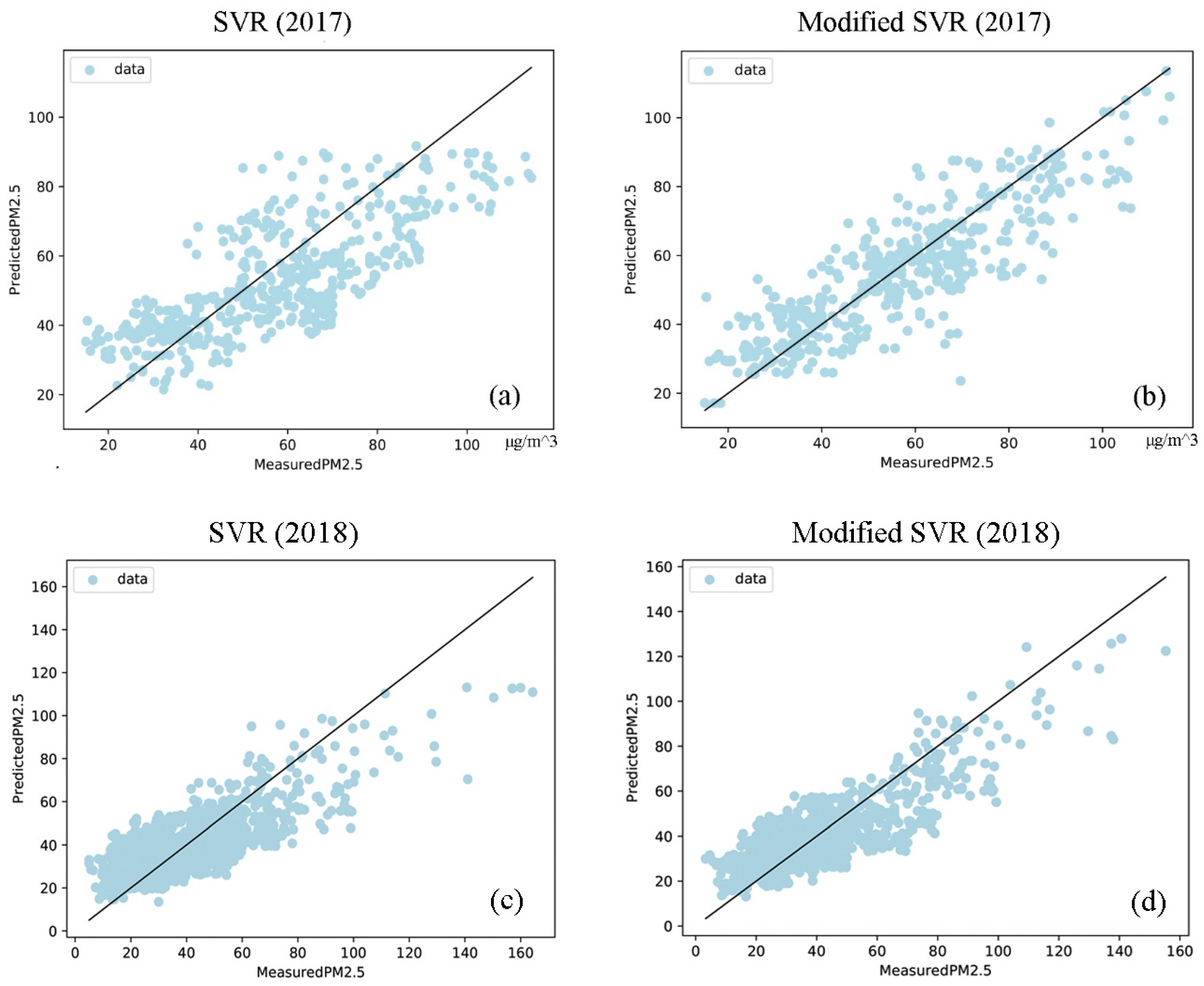
3.1.2. Estimated PM_2.5 by MSVR

Before estimating the PM_2.5 based on the constructed MSVR method, we explored the relationships between PM_2.5 and AOD. The results demonstrated that the AOD had a positive relationship with the PM_2.5 concentrations, and when the site location or observation time changed, the AOD values and PM_2.5 concentrations had similar fluctuating trends. By utilizing the optimal MSVR model produced in the training process, we obtained continuous PM_2.5 estimations at a spatial resolution of 1 km. For visualization, we created a rendering map reflecting the concentration and distribution of PM_2.5 in the study area, which is shown in Figure 3. As shown in the graph, the PM_2.5 estimations had different values and distributions in different regions, and we discuss the details of these features in the following section.

3.2. Pattern Analysis of PM_2.5 Concentrations

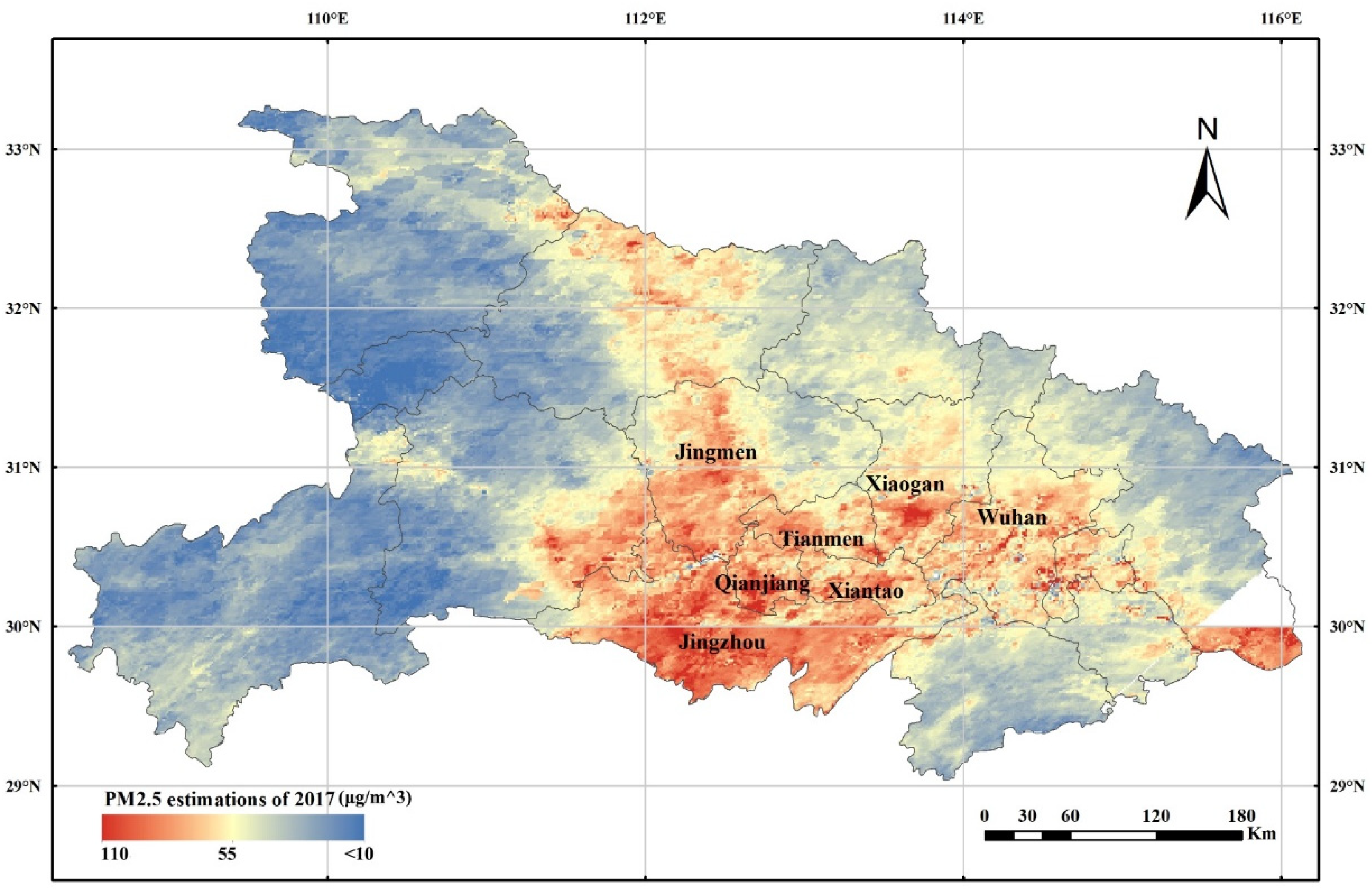
3.2.1. Spatial Pattern of the Estimated PM_2.5

The MSVR model proposed in this paper was used to estimate the continuous PM_2.5 concentrations in the study area at the grid resolutions of both $1\times 1\mathrm{km}$ from the MAIAC AOD and $3\times 3\mathrm{km}$ from the MODIS AOD. Although derived from different data sources, the distribution patterns of MAIAC- and MODIS-derived PM_2.5 were very similar, e.g., similar high-value areas and similar spatial variation patterns.

Whether from MAIAC or MODIS, the high PM_2.5 concentrations generally occurred in developed urban cities where the population and pollution sources were concentrated, while the low PM_2.5 concentrations usually occurred in rural areas or mountainous areas as it was demonstrated in the literature. In the study area of Hubei Province, the high values were mainly distributed in Wuhan, Xiangyang, Jingzhou and other quickly developing cities.

As shown in Figure 4, although the PM_2.5 of MODIS and MAIAC have extremely similar spatial distributions in 2017, the 1 km PM_2.5 from MAIAC has indisputable advantages in terms of resolution. When the study area was zoomed out to a smaller scale, such as an urban area, the 3 km PM_2.5 could describe only the general spatial variation, and the pixels became relatively coarse and difficult to read. However, the 1 km PM_2.5 derived from MAIAC AOD were able to reflect subtler spatial changes and could distinguish the pixels with high levels of PM_2.5 from the others; this difference enabled us to locate the pollution sources.

Additionally, MAIAC AOD with 1 km resolution could generate many more AOD-PM_2.5 pairs [52,53] than MODIS AOD with 3 km resolution. As a result, when the dataset becomes larger, the MAIAC AOD is able to reflect more information related to PM_2.5, and can achieve better results.

To evaluate the estimating accuracy, we extract the measured PM_2.5 values of ground monitoring site 1844A as the situ true values. The estimated PM_2.5 values are generated from MAIAC 1 km AOD and MODIS 3 km AOD. We analyzed the linear correlation of the measured and estimated PM_2.5 values, 0.6355 for MAIAC AOD and 0.5918 for MODIS AOD (shown as Figure 5). As the result shows, the PM_2.5 estimated from MAIAC AOD not only have higher spatial resolution, but also have higher estimating accuracy, which reveals the feasibility and superiority of MAIAC AOD in terms of PM_2.5 estimating.

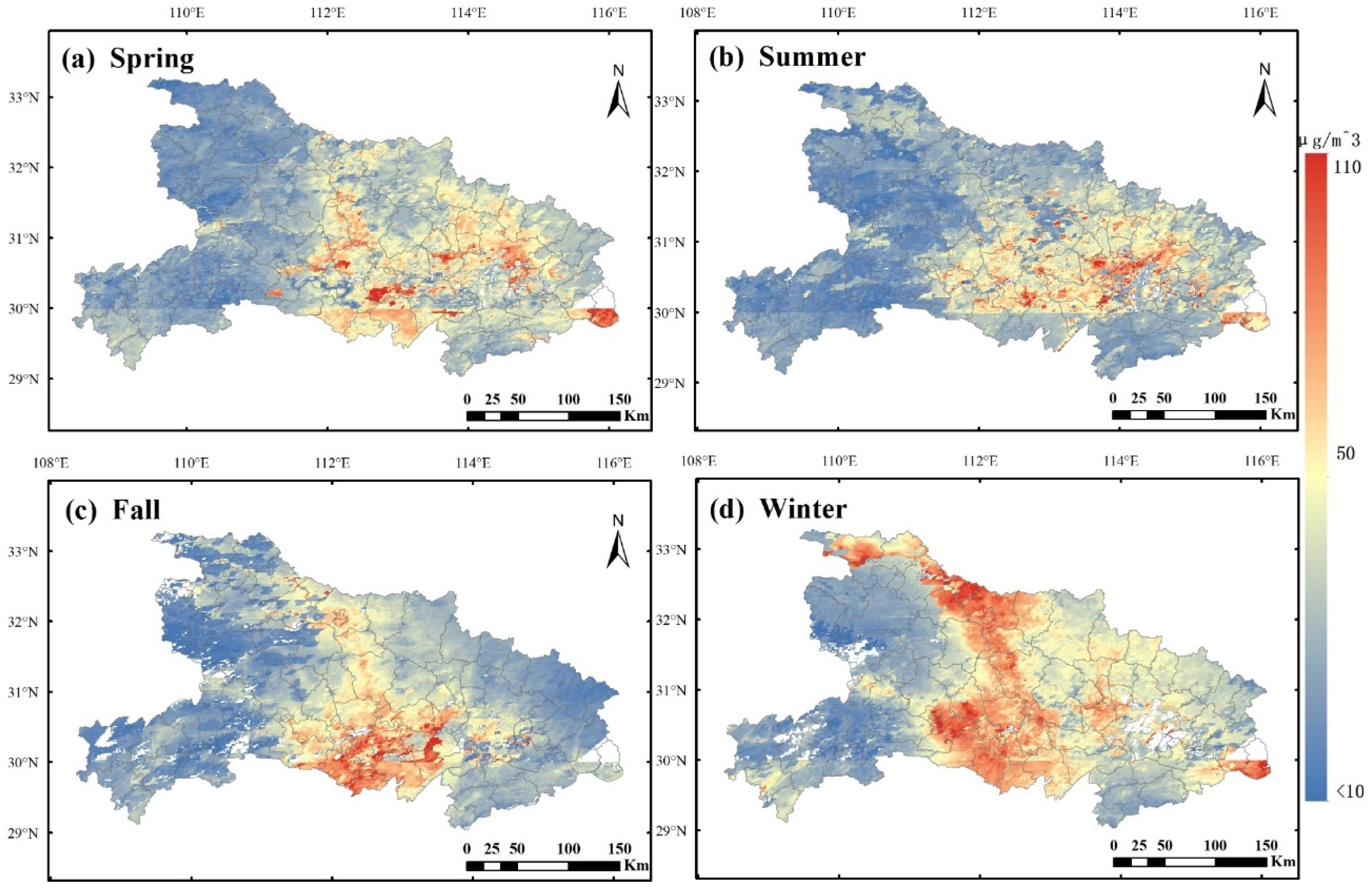
3.2.2. Seasonal Pattern of the Estimated PM_2.5

To illustrate the temporal and seasonal pattern of PM_2.5 in the study area, the data for different seasons were extracted to construct the seasonal regression models and then estimate the PM_2.5 concentrations of different seasons. Figure 6 shows the seasonal mean value distributions of PM_2.5. Figure 6 shows that the PM_2.5 estimations derived from the optimal MSVR model using the 1 km resolution MAIAC AOD values as the model inputs had significant seasonal differences.

The PM_2.5 concentration values were generally low in summer, reaching the lowest values among the four seasons. Conversely, the PM_2.5 concentrations reached the highest level in winter, which might be the reason for more frequent air pollution weather in winter. In addition, the PM_2.5 concentrations in spring and autumn fell between the other two seasons, generally higher than summer and lower than winter, which could be explained by the seasonal climate differences.

The PM_2.5 concentration values were generally low in summer, reaching the lowest values among the four seasons. On the contrary, the PM_2.5 concentrations generally reached the high level in winter, which fitted the fact that the smoggy weather occurred more frequently in winter. Furthermore, from this side, our experiment results were reasonable. In addition, the PM_2.5 concentrations in spring and autumn fell between the other two seasons, generally higher than summer and lower than winter, which could be explained by the seasonal climate differences.

4. Discussion

4.1. Performance of the MSVR Model

Conventional Support Vector Regression (SVR) models were conducted on the same dataset to compare and evaluate the performance of MSVR. Three evaluation indexes, including the R², MPE and RMSE, were applied in the model performance evaluation. As recorded in

Table 4. Accuracy comparisons between SVR and MSVR for different seasons and the entire year in 2017.

Model	Time Period	R2	$\mathbf{MPE}(\mathsf{\mu }\mathbf{g}/{\mathbf{m}}^3)$	$\mathbf{RMSE}(\mathsf{\mu }\mathbf{g}/{\mathbf{m}}^3)$
SVR	Whole year (2017)	0.60	11.16	12.58
	Spring	0.61	12.14	14.53
	Summer	0.50	10.54	12.55
	Autumn	0.56	12.63	15.31
	Winter	0.64	13.35	15.68
Modified SVR (MSVR)	Whole year (2017)	0.74	9.74	10.85
	Spring	0.69	10.69	13.76
	Summer	0.53	8.33	10.36
	Autumn	0.70	10.01	14.02
	Winter	0.82	12.35	14.71

and

Table 5. Accuracy comparisons between SVR and MSVR for different seasons and the entire year in 2018.

Model	Time Period	R2	$\mathbf{MPE}(\mathsf{\mu }\mathbf{g}/{\mathbf{m}}^3)$	$\mathbf{RMSE}(\mathsf{\mu }\mathbf{g}/{\mathbf{m}}^3)$
SVR	Whole year (2018)	0.66	10.11	12.85
	Spring	0.53	11.04	13.66
	Summer	0.52	9.62	11.47
	Autumn	0.60	11.39	13.18
	Winter	0.72	12.65	14.92
Modified SVR (MSVR)	Whole year (2018)	0.78	8.92	11.32
	Spring	0.61	9.58	11.89
	Summer	0.59	8.27	11.01
	Autumn	0.76	10.17	12.22
	Winter	0.80	11.64	12.15

, the regression accuracy was influenced by season and model type and generally increased when models were established in different seasons (e.g., the summer model showed poor performance due to the absence of AOD data) compared to the whole year; additionally, the MSVR model generally had better performance than the SVR. The R² of the whole-year MSVR model increased by 0.14 compared to the SVR model, while the MPE and RMSE of the MSVR model decreased by 1.42 $\mathsf{\mu }\mathrm{g}/{\mathrm{m}}^3$ and 1.73 $\mathsf{\mu }\mathrm{g}/{\mathrm{m}}^3$, respectively. Considering the complexity of atmospheric retrieval and study area, surface reflectance impact, cloud contamination, etc., we think MSVR in this paper obtained relatively good performance.

The R², MPE and RMSE of the MSVR models generally increased in the four seasons, respectively. The measurements and estimation values at different scales for different seasons showed that the PM_2.5 concentration values changed over time. Generally, as the results illustrate, the PM_2.5 concentrations reached a peak value in winter and the lowest value in summer, which was in good agreement with existing empirical knowledge.

As shown in Figure 7, the estimated PM_2.5 and measured PM_2.5 are concentratedly distributed near the centerline, which means that the estimated PM_2.5 generally have the similar pattern with the measured PM_2.5 no matter for MSVR model or SVR model. According to the figure, most of PM_2.5 values fall between 20 $\mathsf{\mu }\mathrm{g}/{\mathrm{m}}^3$ to 80 $\mathsf{\mu }\mathrm{g}/{\mathrm{m}}^3$. And from the figure, the gap between the estimated and measured PM_2.5 values of SVR model gets bigger when PM_2.5 values get higher. This means the MSVR model is more capable for accurate estimating in the high level of PM_2.5 values.

As the results showed, the MSVR model performed better than the conventional SVR model in PM_2.5 estimating. In addition, compared with other nonlinear models, such as the neural network, MSVR is more suitable for relatively small datasets, such as the dataset used in this paper. SVM has a solid mathematical theoretical basis and a strong generalization ability, which can effectively solve the problem of high-dimensional data model construction under limited sample size, and correspondingly, MSVR is relatively easy to construct and train compared to other nonlinear models.

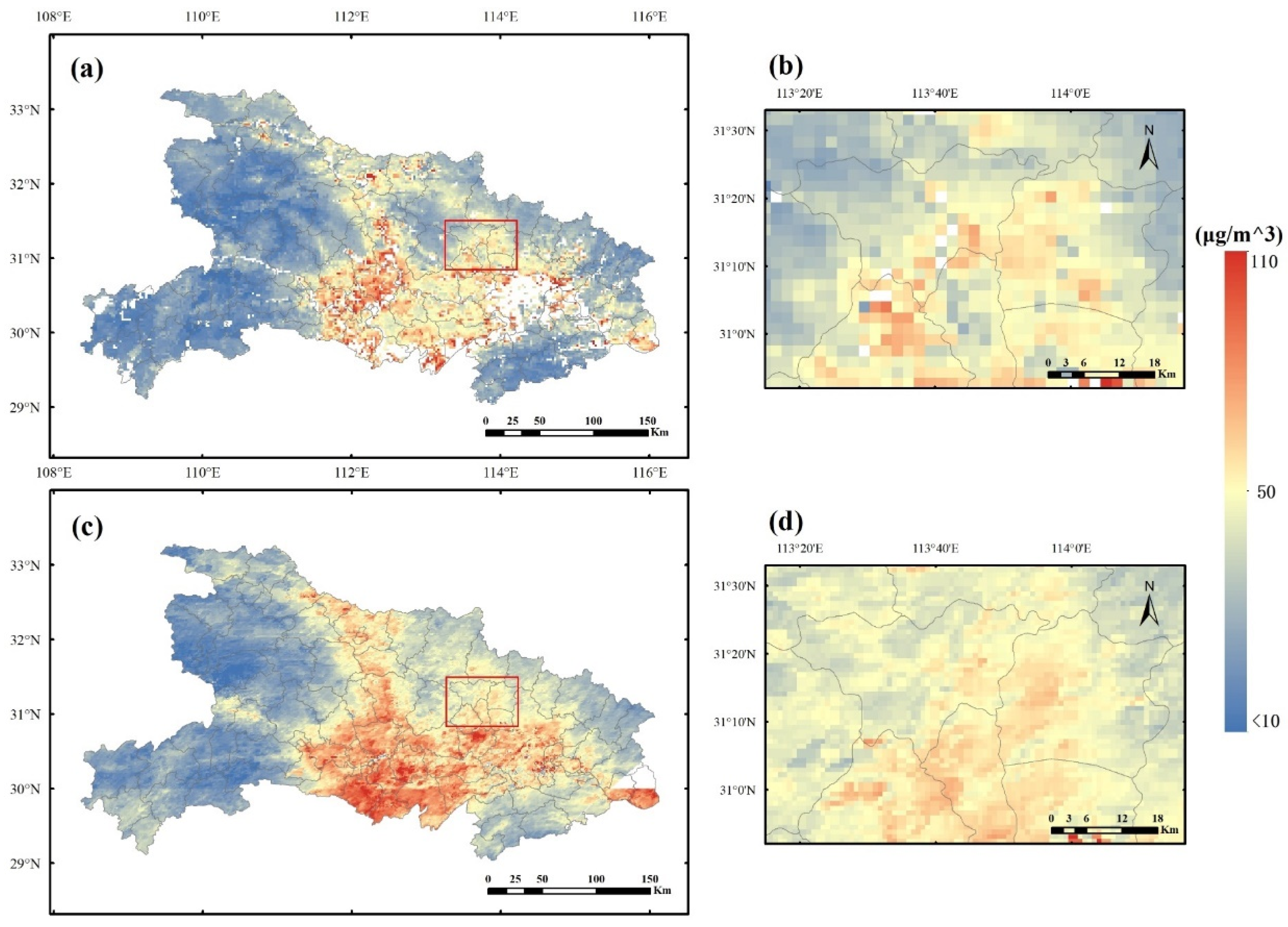
4.2. Advantages of MAIAC AOD

In this paper, the MAIAC AOD with a spatial resolution of 1 km and the MODIS AOD with a spatial resolution of 3 km were utilized to estimate the ambient PM_2.5 concentrations with the same optimal model. According to the results, the PM_2.5 estimations from MAIAC AOD and MODIS AOD had similar spatial and temporal distributions. However, as shown in Figure 4 and Figure 5, MAIAC AOD with 1 km resolution could generate many more AOD-PM_2.5 pairs than MODIS AOD with 3 km resolution. As a result, when the dataset becomes larger, the MAIAC AOD is able to reflect more information related to PM_2.5, and can achieve better results in the inversion. Researches have shown that the correlation between PM_2.5 and AOD decreased significantly as AOD resolution was degraded in spite of the intrinsic mismatch between PM_2.5 ground level measurements and AOD vertically integrated measurements [54]. This conclusion could also be seen from our analysis in Figure 5.

PM_2.5 retrievals of higher spatial resolution make it possible to figure out the spatial distribution characteristics. This is of great importance to accurately locate the source of air pollution where the PM_2.5 concentration usually abnormally elevates. Additionally, we cannot ignore the other superiorities of MAIAC algorithm over the DB/DT algorithm. For example, high-resolution MAIAC is capable to distinguish aerosol sources and fine feature, MAIAC retrieval accuracy is higher than DT/DB with more accuracy over dark surface, and MAIAC has less sensitivity to variation in aerosol types across the seasons.

4.3. Analyses of the Spatiotemporal Pattern of PM_2.5

Firstly, as shown in Figure 3, it should be noted that most cities in the middle and southern parts, such as Jingzhou, Qianjiang, Jingmen, and Wuhan, have the higher PM_2.5 concentration level. This might be interpreted as the lager population, heavy vehicle emissions and more reliance on carbon-intensive industries for a significant proportion of their economic activities [55]. Additionally, researches show that secondary particles resulting from chemical reactions in primary gaseous pollutants may also contribute to levels in this region [51]. On the other hand, the lowest PM_2.5 level occurs in Shiyan, northwest of Hubei, with more mountainous woodland and vegetation cover and far lower anthropogenic emission levels, which is helpful for atmospheric dispersion and dilution.

Secondly, the PM_2.5 concentrations differ greatly across the seasons. The highest PM_2.5 levels in 2017 occurred during the winter and the lowest during the summer (Figure 6). Seasonal maximum PM_2.5 concentrations in winter may be the reason of coal combustion and unfavorable meteorological conditions for pollution dispersion in winter (such as the stagnant weather and temperature inversion) [56]. It is worth noting that the secondary particles generated from chemical reactions in primary gaseous pollutants can contribute to fine PM formation. Summer was the season with the lowest average PM_2.5 concentration. This may be interpreted as the reduced anthropogenic emissions related to coal burning for domestic heating; summer monsoons can also help to dissipate aerosols [57].

4.4. Limitations

The MSVR method proposed in this paper has its own limitations. First, due to the missing AOD data on some days, which are usually caused by cloud cover and high surface reflectance, the number of AOD-PM_2.5 matchups per day is limited [58], resulting in model over-fitting or decreased estimation accuracy. Moreover, the focus of this experiment is the regression method. PM_2.5 feature analyses in large-scale and long period or in the urban areas are not detailed enough. In future work, more available satellite data with higher resolution and quality should be introduced into AOD-PM_2.5 research.

It is worth noting that MODIS AOD is a column average and not surface. There are satellite products that offer vertical profiles, and these are assimilated in MERRA-2 and ECMWF air chemistry sub-models, and could provide surface estimates [59]. However, in view of the current wide application of MODIS AOD and the current research on AOD of vertical profiles not being enough, we have not explored the impact of column average on the experiment. This is the focus of our future work.

In this experiment, we mainly added meteorological and land cover data but, in fact, the relationship between AOD and PM_2.5 is affected by many factors, such as the temperature inversion and more parameters including meteorological, topographic and society parameters [60]. The influence of these factors is relatively complex, and the current research is not yet mature. In future work, we will try to introduce more factors into the regression and analysis.

In addition, the composition and structure of atmospheric pollutants are quite complex and diverse [61], such as SO₂, NO₂, CO, O₃, etc. We will be committed in the research and retrieval of AOD and other more pollutants.

5. Conclusions

The satellite AOD data used in this experiment has superiority over the conventional DB/DT AOD in terms of resolution and accuracy. A higher resolution (1 km) satellite AOD data is used to ensure that the obtained PM_2.5 can reflect more accurate and detailed temporal and spatial characteristics. Additionally, the accuracy of MAIAC algorithm has been proved to be higher than DT/DB algorithm over dark surface. The experiment verified the feasibility of 1 km MAIAC AOD for PM_2.5 retrieval and the superiority over the 3 km MODIS AOD in terms of spatial resolution and retrieval accuracy.

MSVR proposed in this paper, is modified based on the traditional SVR for the regression of AOD and PM_2.5 and obtain the improvement of experiment accuracy. The results showed that the MSVR model could improve the accuracy of the regression from R² 0.60 to 0.74 in 2017 and 0.66 to 0.78 in 2018 compared to the traditional SVR.

We introduced the commonly used meteorological parameters to reduce the influence of complex factors on PM_2.5 retrieval from satellite AOD to a certain extent. The integrated meteorological parameters and land cover data demonstrated that the appropriate auxiliary variables could improve the performance of PM_2.5 retrieval.

The experimental results also showed that PM_2.5 has obvious spatial and temporal differences. We analyzed the spatial and temporal distribution and characteristics of PM_2.5 in Hubei Province, and conducted the above analysis by season. We also analyzed the possible reason of such spatiotemporal differences.

In our future work, we will make efforts from three aspects. First, we will try to find satellites with higher resolution and aerosol retrieval algorithm with better performance. It is worth noting that, recently, there are studies that propose combining satellite remote-sensing techniques and a newly established low-cost sensor network to estimate long-term PM_2.5 concentrations to increase the measurement density. Secondly, we will try to figure out the specific influence of meteorological, topographic and social factors on the distribution characteristics of PM_2.5 and the retrieval of PM_2.5 from satellite AOD. Thirdly, we will attempt to conduct longer time series and wider range of analyses of PM_2.5 distribution characteristics.

References

1. Landrigan, P.J.; Fuller, R.; Acosta, N.J.R.; Adeyi, O.; Arnold, R.; Basu, N.; Baldé, A.B.; Bertollini, R.; Bose-O’Reilly, S.; Boufford, J.I.; et al. The Lancet Commission on pollution and health. Lancet 2018, 391, 462–512. [Google Scholar] [CrossRef] [Green Version]
2. Beelen, R.; Raaschou-Nielsen, O.; Stafoggia, M.; Andersen, Z.J.; Weinmayr, G.; Hoffmann, B.; Wolf, K.; Samoli, E.; Fischer, P.; Nieuwenhuijsen, M.J.; et al. Effects of long-term exposure to air pollution on natural-cause mortality: An analysis of 22 European cohorts within the multicentre ESCAPE project. Lancet 2014, 383, 785–795. [Google Scholar] [CrossRef]
3. Polezer, G.; Tadano, Y.S.; Siqueira, H.V.; Godoi, A.F.; Yamamoto, C.I.; De André, P.A.; Pauliquevis, T.; Andrade, M.D.F.; Oliveira, A.; Saldiva, P.H.; et al. Assessing the impact of PM2.5 on respiratory disease using artificial neural networks. Environ. Pollut. 2018, 235, 394–403. [Google Scholar] [CrossRef] [PubMed]
4. Chan, Y.C.; Simpson, R.W.; Mctainsh, G.H.; Vowles, P.D.; Cohen, D.D. Characterisation of chemical species in PM2.5 and PM10 aerosols in Brisbane, Australia. Atmos. Environ. 2015, 37, 31–39. [Google Scholar] [CrossRef]
5. Wang, Y.; Jia, C.; Tao, H.; Zhang, L.; Liang, X.; Ma, J.-M.; Gao, H.; Huang, T.; Zhang, K. Chemical characterization and source apportionment of PM2.5 in a semi-arid and petrochemical-industrialized city, Northwest China. Sci. Total Environ. 2016, 573, 1031–1040. [Google Scholar] [CrossRef] [PubMed]
6. Ma, Z.; Hu, X.; Sayer, A.M.; Levy, R.; Zhang, Q.; Xue, Y.; Tong, S.; Bi, J.; Huang, L.; Liu, Y. Satellite-based spatiotem-poral trends in PM2. 5 concentrations: China. Environ. Health Perspect. 2016, 124, 184–192. [Google Scholar] [CrossRef] [PubMed] [Green Version]
7. Li, S.; Joseph, E.; Min, Q. Remote sensing of ground-level PM2.5 combining AOD and backscattering profile. Remote Sens. Environ. 2016, 183, 120–128. [Google Scholar] [CrossRef]
8. Paciorek, C.J.; Yang, L. AOD–PM2.5 Association: Paciorek and Liu Respond. Environ. Health Perspect. 2010, 118, A110–A111. [Google Scholar] [CrossRef] [Green Version]
9. Zhang, T.; Gong, W.; Wang, W.; Ji, Y.; Zhu, Z.; Huang, Y. Ground Level PM2.5 Estimates over China Using Satellite-Based Geographically Weighted Regression (GWR) Models Are Improved by Including NOâ‚‚ and Enhanced Vegetation Index (EVI). Int. J. Environ. Res. Public Health 2016, 13, 1215. [Google Scholar] [CrossRef]
10. Wei, J.; Huang, W.; Li, Z.; Xue, W.; Peng, Y.; Sun, L.; Cribb, M. Estimating 1-km-resolution PM2.5 concentrations across China using the space-time random forest approach. Remote Sens. Environ. 2019, 231, 111221. [Google Scholar] [CrossRef]
11. Xia, X.; Qi, Q.; Liang, H.; Zhang, A.; Jiang, L.; Ye, Y.; Liu, C.; Huang, Y. Pattern of spatial distribution and tem-poral variation of atmospheric pollutants during 2013 in Shenzhen, China. ISPRS Int. J. Geoinf. 2017, 6, 2. [Google Scholar] [CrossRef]
12. Gross, B.; Schäfer, K.; Keckhut, P. Special Section Guest Editorial: Advances in Remote Sensing for Air Quality Management. J. Appl. Remote Sens. 2018, 12, 042601. [Google Scholar] [CrossRef] [Green Version]
13. Park, S.; Choi, J. Satellite-measured atmospheric aerosol content in Korea: Anthropogenic signals from decadal records. GISci. Remote Sens. 2016, 53, 1–17. [Google Scholar] [CrossRef]
14. Yuanyu, X.; Yuxuan, W.; Kai, Z.; Wenhao, D.; Baolei, L.; Yuqi, B. Daily Estimation of Ground-Level PM2.5 Concentrations over Beijing Using 3 km Resolution MODIS AOD. Environ. Sci. Technol. 2015, 49, 12280–12288. [Google Scholar]
15. You, W.; Zang, Z.; Zhang, L.; Li, Y.; Wang, W. Estimating national-scale ground-level PM25 concentration in China using geographically weighted regression based on MODIS and MISR AOD. Environ. Sci. Pollut. Res. 2016, 23, 8327–8338. [Google Scholar] [CrossRef]
16. You, W.; Zang, Z.; Pan, X.; Zhang, L.; Chen, D. Estimating PM2.5 in Xi’an, China using aerosol optical depth: A comparison between the MODIS and MISR retrieval models. Sci. Total. Environ. 2015, 505, 1156–1165. [Google Scholar] [CrossRef]
17. Zang, L.; Mao, F.; Guo, J.; Gong, W.; Wang, W.; Pan, Z. Estimating hourly PM1 concentrations from Himawari-8 aerosol optical depth in China. Environ. Pollut. 2018, 241, 654–663. [Google Scholar] [CrossRef]
18. Yumimoto, K.; Nagao, T.M.; Kikuchi, M.; Sekiyama, T.T.; Murakami, H.; Tanaka, T.Y.; Ogi, A.; Irie, H.; Khatri, P.; Okumura, H. Aerosol data assimilation using data from Himawari-8, a next-generation geostationary meteorological satellite: Aero-sol assimilation with Himawari-8. Geophys. Res. Lett. 2016, 43, 5886–5894. [Google Scholar] [CrossRef]
19. Yao, F.; Si, M.; Li, W.; Wu, J. A multidimensional comparison between MODIS and VIIRS AOD in estimating ground-level PM2.5 concentrations over a heavily polluted region in China. Sci. Total Environ. 2018, 618, 819–828. [Google Scholar] [CrossRef]
20. Mhawish, A.; Banerjee, T.; Sorek-Hamer, M.; Lyapustin, A.; Broday, D.M.; Chatfield, R. Comparison and evaluation of MODIS Multi-angle Implementation of Atmospheric Correction (MAIAC) aerosol product over South Asia. Remote Sens. Environ. 2019, 224, 12–28. [Google Scholar] [CrossRef]
21. Lyapustin, A.; Wang, Y.; Korkin, S.; Huang, D. MODIS Collection 6 MAIAC algorithm. Atmos. Meas. Tech. 2018, 11, 5741–5765. [Google Scholar] [CrossRef] [Green Version]
22. Boyouk, N.; Léon, J.-F.; Delbarre, H.; Podvin, T.; DeRoo, C. Impact of the mixing boundary layer on the relationship between PM2.5 and aerosol optical thickness. Atmos. Environ. 2010, 44, 271–277. [Google Scholar] [CrossRef]
23. Zheng, C.; Zhao, C.; Zhu, Y.; Wang, Y.; Shi, X.; Wu, X.; Chen, T.; Wu, F.; Qiu, Y. Analysis of influential factors for the relationship between PM2.5 and AOD in Beijing. Atmos. Chem. Phys. Discuss. 2017, 17, 13473–13489. [Google Scholar] [CrossRef] [Green Version]
24. Ma, Z.; Hu, X.; Huang, L.; Bi, J.; Liu, Y. Estimating Ground-Level PM2.5 in China Using Satellite Remote Sensing. Environ. Sci. Technol. 2014, 48, 7436–7444. [Google Scholar] [CrossRef] [PubMed]
25. Guo, J.; Xia, F.; Zhang, Y.; Liu, H.; Li, J.; Lou, M.; He, J.; Yan, Y.; Wang, F.; Min, M.; et al. Impact of diurnal variability and meteorological factors on the PM2.5—AOD relationship: Implications for PM2.5 remote sensing. Environ. Pollut. 2017, 221, 94–104. [Google Scholar] [CrossRef] [Green Version]
26. Liu, Y.; Paciorek, C.J.; Koutrakis, P. Estimating Regional Spatial and Temporal Variability of PM 2.5 Concentrations Using Satellite Data, Meteorology, and Land Use Information. Environ. Health Perspect. 2009, 117, 886–892. [Google Scholar] [CrossRef] [Green Version]
27. Xiao, L.; Lang, Y.; Christakos, G.J.A.E. High-resolution spatiotemporal mapping of PM2. 5 concentrations at Mainland Chi-na using a combined BME-GWR technique. Atmos. Environ. 2018, 173, 295–305. [Google Scholar] [CrossRef]
28. Zhai, L.; Li, S.; Zou, B.; Sang, H.; Fang, X.; Xu, S. An improved geographically weighted regression model for PM 2.5 concentration estimation in large areas. Atmos. Environ. 2018, 181, 145–154. [Google Scholar] [CrossRef]
29. Su, T.; Li, J.; Li, C.; Lau, A.K.-H.; Yang, D.; Shen, C. An intercomparison of AOD-converted PM2.5 concentrations using different approaches for estimating aerosol vertical distribution. Atmos. Environ. 2017, 166, 531–542. [Google Scholar] [CrossRef]
30. Chen, G.; Li, S.; Knibbs, L.D.; Hamm, N.; Cao, W.; Li, T.; Guo, J.; Ren, H.; Abramson, M.J.; Guo, Y. A machine learning method to estimate PM2.5 concentrations across China with remote sensing, meteorological and land use information. Sci. Total Environ. 2018, 636, 52–60. [Google Scholar] [CrossRef]
31. Yang, Q.; Yuan, Q.; Yue, L.; Li, T.; Shen, H.; Zhang, L. The relationships between PM2.5 and aerosol optical depth (AOD) in mainland China: About and behind the spatio-temporal variations. Environ. Pollut. 2019, 248, 526–535. [Google Scholar] [CrossRef] [PubMed]
32. Yang, W.; Deng, M.; Xu, F.; Wang, H. Prediction of hourly PM2.5 using a space-time support vector regression model. Atmos. Environ. 2018, 181, 12–19. [Google Scholar] [CrossRef]
33. Roy, A.; Chakraborty, S. Support vector regression based metamodel by sequential adaptive sampling for reliability analysis of structures. Reliab. Eng. Syst. Saf. 2020, 200, 106948. [Google Scholar] [CrossRef]
34. Zhang, T.; Zhu, Z.; Gong, W.; Zhu, Z.; Sun, K.; Wang, L.; Huang, Y.; Mao, F.; Shen, H.; Li, Z.; et al. Estimation of ultrahigh resolution PM2.5 concentrations in urban areas using 160 m Gaofen-1 AOD retrievals. Remote Sens. Environ. 2018, 216, 91–104. [Google Scholar] [CrossRef]
35. Giles, D.M.; Sinyuk, A.; Sorokin, M.G.; Schafer, J.S.; Smirnov, A.; Slutsker, I.; Eck, T.F.; Holben, B.N.; Lewis, J.R.; Campbell, J.R. Advancements in the Aerosol Robotic Network (AERONET) Version 3 database–automated near-real-time quality control algorithm with improved cloud screening for Sun photometer aerosol optical depth (AOD) measurements. Atmos. Meas. Tech. 2019, 12, 169–209. [Google Scholar] [CrossRef] [Green Version]
36. Zhang, Z.; Wu, W.; Fan, M.; Wei, J.; Tan, Y.; Wang, Q. Evaluation of MAIAC aerosol retrievals over China. Atmos. Environ. 2019, 202, 8–16. [Google Scholar] [CrossRef]
37. Chen, G.; Knibbs, L.D.; Zhang, W.; Li, S.; Cao, W.; Guo, J.; Ren, H.; Wang, B.; Wang, H.; Williams, G. Estimating spatiotem-poral distribution of PM1 concentrations in China with satellite remote sensing, meteorology, and land use information. Environ. Pollut. 2018, 233, 1086–1094. [Google Scholar] [CrossRef]
38. Wang, J.; Ogawa, S. Effects of Meteorological Conditions on PM2.5 Concentrations in Nagasaki, Japan. Int. J. Environ. Res. Public Health 2015, 12, 9089–9101. [Google Scholar] [CrossRef]
39. Huang, F.; Xia, L.; Chao, W.; Qin, X.; Wei, W.; Luo, Y.; Tao, L.; Qi, G.; Jin, G.; Chen, S.; et al. PM2.5 Spatiotemporal Variations and the Relationship with Meteorological Factors during 2013-2014 in Beijing, China. PLoS ONE 2015, 10, e0141642. [Google Scholar] [CrossRef]
40. Trifonova, T.A.; Mishchenko, N.V.; Grishina, Y.P. A remote sensing-based method for determining industrial air pollution. Mapp. Sci. Remote Sens. 1998, 35, 22–30. [Google Scholar] [CrossRef]
41. Chen, B.; Li, S.; Yang, X.; Lu, S.; Wang, B.; Niu, X. Characteristics of atmospheric PM2.5 in stands and non-forest cover sites across urban-rural areas in Beijing, China. Urban Ecosyst. 2016, 19, 867–883. [Google Scholar] [CrossRef]
42. Kumar, A. Long term (2003–2012) spatiotemporal MODIS (Terra/Aqua level 3) derived climatic variations of aerosol opti-cal depth and cloud properties over a semiarid urban tropical region of Northern India. Atmos. Environ. 2014, 83, 291–300. [Google Scholar] [CrossRef]
43. Hao, Y.; Liu, Y. The influential factors of urban PM2.5 concentrations in China: A spatial econometric analysis. J. Clean. Prod. 2016, 112, 1443–1453. [Google Scholar] [CrossRef]
44. Kelly, K.M.; Dennis, M.L. Transforming between WGS84 Realizations and other Reference Frames. In AGU Fall Meeting Abstracts; American Geophysical Union: Washington, DC, USA, 2018. [Google Scholar]
45. Noble, W. What is a support vector machine? Nat. Biotechnol. 2006, 24, 1565–1567. [Google Scholar] [CrossRef] [PubMed]
46. Smola, A.J.; Schölkopf, B. A tutorial on support vector regression. Stat. Comput. 2004, 14, 199–222. [Google Scholar] [CrossRef] [Green Version]
47. Chang, C.-C.; Lin, C.-J. LIBSVM: A library for support vector machines. ACM Trans. Intell. Syst. Technol. 2011, 2, 27. [Google Scholar] [CrossRef]
48. Zhu, S.; Lian, X.; Wei, L.; Che, J.; Shen, X.; Yang, L.; Qiu, X.; Liu, X.; Gao, W.; Ren, X.; et al. PM2.5 forecasting using SVR with PSOGSA algorithm based on CEEMD, GRNN and GCA considering meteorological factors. Atmos. Environ. 2018, 183, 20–32. [Google Scholar] [CrossRef]
49. Awad, M.; Khanna, R. Support vector regression. In Efficient Learning Machines; Apress: Berkeley, CA, USA, 2015; pp. 67–80. [Google Scholar]
50. Wang, S.; Zhou, C.; Wang, Z.; Feng, K.; Hubacek, K. The characteristics and drivers of fine particulate matter (PM2.5) distribution in China. J. Clean. Prod. 2017, 142, 1800–1809. [Google Scholar] [CrossRef]
51. Balasundaram, S. On Lagrangian support vector regression. Expert Syst. Appl. 2010, 37, 8784–8792. [Google Scholar] [CrossRef]
52. Chudnovsky, A.; Tang, C.; Lyapustin, A.; Wang, Y.; Schwartz, J.; Koutrakis, P.J.A.C. A critical assessment of high-resolution aerosol optical depth retrievals for fine particulate matter predictions. Atmos. Chem. Phys. 2013, 13, 10907. [Google Scholar] [CrossRef] [Green Version]
53. Chudnovsky, A.A.; Koutrakis, P.; Kloog, I.; Melly, S.J.; Nordio, F.; Lyapustin, A.I.; Wang, Y.; Schwartz, J. Fine particulate matter predictions using high resolution Aerosol Optical Depth (AOD) retrievals. Atmos. Environ. 2014, 89, 189–198. [Google Scholar] [CrossRef] [Green Version]
54. Chudnovsky, A.A.; Kostinski, A.; Lyapustin, A.; Koutrakis, P.J.E.P. Spatial scales of pollution from variable resolution satellite imaging. Environ. Pollut. 2013, 172, 131–138. [Google Scholar] [CrossRef] [PubMed]
55. Guan, D.; Su, X.; Zhang, Q.; Peters, G.P.; Liu, Z.; Lei, Y.; He, K. The socioeconomic drivers of China’s primary PM 2.5 emissions. Environ. Res. Lett. 2014, 9, 024010. [Google Scholar] [CrossRef] [Green Version]
56. Huang, T.; Yu, Y.; Wei, Y.; Wang, H.; Huang, W.; Chen, X. Spatial–seasonal characteristics and critical impact factors of PM2. 5 concentration in the Beijing–Tianjin–Hebei urban agglomeration. PLoS ONE 2018, 13, e0201364. [Google Scholar]
57. Cheng, Z.; Li, L.; Liu, J. Identifying the spatial effects and driving factors of urban PM2.5 pollution in China. Ecol. Indic. 2017, 82, 61–75. [Google Scholar] [CrossRef]
58. Lin, C.; Labzovskii, L.; Mak, H.W.L.; Fung, J.C.; Lau, A.K.; Kenea, S.T.; Bilal, M.; Hey, J.D.V.; Lu, X.; Ma, J. Observation of PM2.5 using a combination of satellite remote sensing and low-cost sensor network in Siberian urban areas with limited reference monitoring. Atmos. Environ. 2020, 227, 117410. [Google Scholar] [CrossRef]
59. Toth, T.D.; Zhang, J.; Campbell, J.R.; Hyer, E.; Reid, J.S.; Shi, Y.; Westphal, D.L. Impact of data quality and surface-to-column representativeness on the PM2.5/satellite AOD relationship for the contiguous United States. Atmos. Chem. Phys. Discuss. 2014, 14, 6049–6062. [Google Scholar] [CrossRef] [Green Version]
60. Zang, Z.; Wang, W.; You, W.; Li, Y.; Ye, F.; Wang, C. Estimating ground-level PM2.5 concentrations in Beijing, China using aerosol optical depth and parameters of the temperature inversion layer. Sci. Total. Environ. 2017, 575, 1219–1227. [Google Scholar] [CrossRef]
61. Lalitaporn, P.; Kurata, G.; Matsuoka, Y.; Thongboonchoo, N.; Surapipith, V.J. Long-term analysis of no 2, co, and aod seasonal variability using satellite observations over asia and intercomparison with emission inventories and model. Atmos. Health 2013, 6, 655–672. [Google Scholar] [CrossRef]
Figure 1. The study area and the monitoring sites were distributed in Hubei Province, and the total number of monitoring sites was 47 at 2017.
Ijgi 10 00031 g001
Figure 2. The main structure of the MSVR model.
Ijgi 10 00031 g002
Figure 3. The estimated PM2.5 average concentrations in the study area in 2017, with the selected optimal MSVR model at spatial resolutions of 1 km.
Ijgi 10 00031 g003
Figure 4. Spatial resolution comparison of the annual 1 km PM2.5 derived from MAIAC AOD (a) and 3 km PM2.5 derived from MODIS AOD (c) in Hubei Province in 2017. When the map is zoomed to a smaller scale, the spatial advantages of the 1 km PM2.5 are displayed by comparing the MAIAC-derived (b) and MODIS-derived (d) PM2.5 concentrations.
Ijgi 10 00031 g004
Figure 5. Linear Correlation Analysis of measured PM2.5 and estimated PM2.5, the estimated PM2.5 are retrieved from MAIAC 1 km AOD and MODIS 3 km AOD.
Ijgi 10 00031 g005
Figure 6. The distribution of and variation in averaged PM2.5 estimations in four seasons (a) for spring, (b) for summer, (c) for autumn, and (d) for winter) in the study area of Hubei, China.
Ijgi 10 00031 g006
Figure 7. The scatterplots of cross validation results for SVR (a) and Modified SVR (b) models in 2017, SVR (c) and Modified Scheme 2018. (d) are shown in the figure. The horizontal axis represents the measured true PM2.5 values and the vertical axis represents the predicted PM2.5 obtained from the regression models. The black lines are the 1:1 reference line.
Ijgi 10 00031 g007