


Abstract
The Mongolian Plateau (MP) experienced the most severe decadal drought of the past two millennia from 2000 to 2009 and several shorter-term droughts in the 2010s. Using satellite-based near-infrared reflectance of vegetation ( ), we examined changes in vegetation productivity of the MP from 2000 to 2018. During this time, soil moisture in March (
 ) mainly determined spring
  , and early-summer (June and July) precipitation mainly determined summer
  Our study revealed three distinct periods: the severely dry period of 2000–2009, recovery in 2010–2012, and a relatively stable period with occasional short-term droughts after 2012. While vegetation productivity experienced a significant decrease during the severe decadal drought, summer and spring productivity quickly recovered after 2010, following an increase in growing season (GS) rainfall and winter snowfall. Greater
  , which resulted from previous GS precipitation, contributed to smaller declines in vegetation productivity during the short-term droughts in 2014, 2015 and 2017. The decline in vegetation productivity during the severe decadal drought damaged livestock operations in Mongolia, but had a limited effect on operations in Inner Mongolia of China, where human intervention is stronger. Given evidence that drought impacts are increasing worldwide, it is important to understand the factors determining ecosystem drought responses. Many drought studies have focused on GS precipitation, but our results show that pre-GS SM can play an important role in determining drought impacts. Our results also demonstrate that strong interventions will be needed in order to sustain livestock operations during intensifying drought.
Export citation and abstract BibTeX RIS

Original content from this work may be used under the terms of the Creative Commons Attribution 4.0 license. Any further distribution of this work must maintain attribution to the author(s) and the title of the work, journal citation and DOI.
1. Introduction
Grasslands cover up to 59 million km2, or over 40% of the global land surface, primarily in arid and semi-arid regions (Suttie et al 2005). They store about 34% of the global terrestrial carbon stock and play a dominant role in global carbon cycle (Field et al 1998, Ahlstrom et al 2015, Lei et al 2020). Grassland vegetation growth and production are largely determined by precipitation (Knapp and Smith 2001, Knapp et al 2002, Peng et al 2013), have large inter-annual variability (Knapp and Smith 2001, Huxman et al 2004), and are known to be vulnerable to drought (Gilgen and Buchmann 2009, Scott et al 2010, Knapp et al 2015). Drought as a widespread hydroclimatic anomaly can be particularly disastrous for grassland ecosystems. As meat and dairy industries are deeply reliant on grassland vegetation productivity to maintain livestock (Nardone et al 2010, O'Mara 2012), drought-induced reductions in vegetation production will cause substantial economic losses. It is thus important to understand how grasslands respond to drought and recover after drought, especially as terrestrial drought impacts have increased and the frequency and intensity of droughts are predicted to continue increasing worldwide with climate change (IPCC 2013, Du et al 2018, Groisman et al 2018).
Long-term observations and many experiments have demonstrated the dominant role of precipitation in determining grassland productivity (Heisler-White et al 2008, Petrie et al 2018). For example, it is well established that reductions in ecosystem productivity are closely associated with the severity of precipitation deficit during dry periods (Nandintsetseg and Shinoda 2013, Wang et al 2019); that different ecosystem and plant functional types (for instance, C3 vs. C4 grasses) may show different responses to drought (Knapp et al 2015, 2020, Piao et al 2019), and that changes in the timing and size of precipitation events can alter vegetation productivity independent of precipitation amount (Knapp et al 2002, Felton et al 2020). However, our current understanding of the factors controlling or modifying ecosystem responses to drought is still limited (Porporato et al 2001, Chaves et al 2002, 2003, van der Molen et al 2011), due in part to the lack of a consensus definition of 'drought' (Slette et al 2019). Our study sought to improve understanding of three important questions: (a) how does the seasonal climate before and during drought influence the response of vegetation to drought, (b) what climatic variables determine that rate of vegetation recovery after drought, and (c) how do drought-induced changes in vegetation productivity affect the livestock industry?
The Mongolian Plateau (MP), including Inner Mongolia (IM) of China and the Republic of Mongolia (Mongolia; MN) (figure S1, which is available online at stacks.iop.org/ERL/16/014050/mmedia), is a semi-arid region with annual precipitation ranging from 230 mm yr−1 to 380 mm yr−1. Much of this region is agricultural rangeland used for herding livestock (Angerer et al
2008). We used long-term climate records and standardized climate indices to identify drought periods in this region. A decadal drought lasting from 2000 to 2009 was the most severe drought in the MP during the past two millennia (Hessl et al
2018), and shorter-term droughts occurred in 2014, 2015, and 2017. We then used a satellite-based vegetation index, near-infrared reflectance of vegetation ( ), as a proxy of vegetation productivity to assess the Mongolian grassland ecosystem response to the long-term and short-term drought periods. We also investigated post-drought recovery of vegetation productivity. We analyzed key environmental variables driving seasonal vegetation productivity during and after both long-term and short-term droughts. Finally, we used livestock sector statistical data from the National Statistical Offices of Mongolia and China to investigate the impacts of long-term and short-term droughts on animal husbandry in these two regions. Our study thus provides insights into the factors that determine the impacts of drought on grasslands vegetation productivity and the livestock sector.
2. Materials and methods
2.1. Data
2.1.1. Vegetation indices and land cover map
Monthly  was derived from the monthly maximum total scene NIR reflectance (NIRT) and normalized difference vegetation index (NDVI) from the MOD13A2 V6 with temporal resolution of 16 d and spatial resolution of 1 km × 1 km (Badgley et al
2017).
was derived from the monthly maximum total scene NIR reflectance (NIRT) and normalized difference vegetation index (NDVI) from the MOD13A2 V6 with temporal resolution of 16 d and spatial resolution of 1 km × 1 km (Badgley et al
2017).  is the product of NIRT and NDVI (Badgley et al
2017). Previous study has shown that
is the product of NIRT and NDVI (Badgley et al
2017). Previous study has shown that  is less influenced by soil reflectance and better related to Gross Primary Production (GPP) than NDVI (Badgley et al
2017).
is less influenced by soil reflectance and better related to Gross Primary Production (GPP) than NDVI (Badgley et al
2017).
In this study, vegetation growing season (GS) is from April to October (Zhou et al
2001, Piao et al
2011), and the GS is divided into three sub-seasons: spring (April and May, AM), summer (June to August, JJA), and autumn (September and October, SO). Variables (e.g.  , SM and T etc) are noted with superscript of seasons. We also used NDVI as a supplementary vegetation productivity index (Peng et al
2011). Pixels with mean annual NDVI less than 0.1 were masked as non-vegetated areas. Then, 1 km × 1 km
, SM and T etc) are noted with superscript of seasons. We also used NDVI as a supplementary vegetation productivity index (Peng et al
2011). Pixels with mean annual NDVI less than 0.1 were masked as non-vegetated areas. Then, 1 km × 1 km  and NDVI were aggregated into 0.1° ×0.1° by average in order to be analyzed with other datasets.
The land cover map derived from MCD12Q1 following the International Geosphere-Biosphere Programme land cover classification scheme (Friedl and Sulla-Menashe 2019) is at a spatial resolution of 500 m and at an annual time step for the period 2001–2018. The land cover types were aggregated into five major classes: forests, shrublands, grasslands, croplands, and others (table S1). Within the 0.1° × 0.1° grids, more than 60% were identified as grids of grasslands and shrublands. We focused on grids that had been persistent as either grasslands or shrublands throughout the study period. Because of the concern on the accuracy of the MODIS landcover product during 2001–2002 (Sulla-Menashe et al 2019), we also implemented the same method on the period 2003–2018 and compared the result with the original 2001–2018 mask. As figures S9 and S10 shows, the two masks are almost the same; hence hereafter we reported results based on the former landcover mask (2001–2018).
2.1.2. Climate and drought indices data
Monthly temperature (T) and precipitation (P) data from the Climate Research Unit (CRU) from 2000 to 2018 with spatial resolution of 0.5° × 0.5° (New et al 2000) were used for this study. We also used Multi-Source Weighted-Ensemble Precipitation (MSWEP) monthly precipitation with spatial resolution of 0.25° × 0.25° to assess precipitation data uncertainty (Beck et al 2017). The monthly snow water equivalent (SWE) data that we used are from the European Space Agency's Global Snow Monitoring for Climate Research (GlobSnow) version 2, covering 1979–2016 with spatial resolution of 25 km (Larue et al 2017). We used the maximum monthly SWE (SWE maximum) between last November and April to indicate available water from snow. The monthly variation of SWE shows consistence with that of the snow cover data from MODIS product (MOD10CM) (figure S8). The self-calibrating Palmer Drought Severity Index (scPDSI) and the (SPEI) were calculated from the CRU TS 4.03 datasets with spatial resolution of 0.5° × 0.5° for 1901–2018 (Wells et al 2004, Vicente-Serrano et al 2010). The 12 month scale SPEI was selected to show the annual variation of moisture deficit.
2.1.3. Soil moisture and terrestrial water storage data
The monthly root-zone soil moisture (SM) data were derived from Global Land Evaporation Amsterdam Model (GLEAM) v3.3a with spatial resolution of 0.25° × 0.25° (Martens et al 2017). The terrestrial water storage (TWS) data from the satellites of the Gravity Recovery and Climate Experiment (GRACE) measures the variation of water storage including groundwater, SM, surface water, snow water, and vegetation water. Here, we used the reconstructed monthly TWS data with a spatial resolution of 0.5° × 0.5° by a model trained with GRACE observations and driven by climate from ERA5 dataset covering the period 1979–2019 (Humphrey and Gudmundsson 2019).
2.1.4. Livestock data
We collected historical annual census data of livestock number and livestock products (milk and meat) to explore the impacts of drought on livestock. For MN, the livestock number in each Aimag (an administrative unit in MN comparable to 'province' in China or 'state' in the U.S.) comes from the National Statistical Offices of Mongolia and the product quantity from the Food and Agriculture Organization (FAO). For IM, both are obtained from the China Statistical Yearbook. The livestock number consist of five main livestock types (horse, cattle, camel, sheep, and goat), and the total livestock number is measured by livestock unit (LU), which is calculated using the livestock number and the specific coefficient from FAO (e.g. 0.65, 0.65, 0.8, 0.1 and 0.1 LU per head for horse, cattle, camel, sheep, and goat, respectively).
2.2. Statistical analyses
Pearson correlation and regression analysis were performed to understand relationships between  and environmental factors, as well as the impacts of drought on animal husbandry. An unpaired t-test was used to determine whether mean annual precipitation differed significantly (p < 0.05) between the two time periods (2000–2009 vs.1950–1999). All statistical analyses were performed using MATLAB R2019a software.
3. Results
3.1. Droughts from 2000 to 2018 in the Mongolian Plateau
The decadal severe drought was identified by precipitation data and two drought indices (the 12 month SPEI12, and the scPDSI) (figure 1). The average annual precipitation in 2000–2009 was 14% lower than that in 1950–1999, 42.5 mm, and the difference is statistically significant (p = 0.0002). Both SPEI12 and scPDSI indicate drought (SPEI12 < −0.5, scPDSI < −1) in most years of 2000–2009 for this region. Moreover, satellite-based TWS, showed a declining trend during the decadal drought (figure 1(c)). This drought was alleviated by increased precipitation and decreased temperature in the 2010s (figure 1). Then, based on annual precipitation records from CRU, short-term droughts revisited the MP in 2014 (262 mm yr−1), 2015 (260 mm yr−1) and 2017 (236 mm yr−1), which are close to the mean annual precipitation during the 2000–2009 drought (259 mm yr−1). Both SPEI12 and scPDSI confirm these short-term droughts in the 2010s (figure 1(c)). The long-term and short-term drought pattern in the two sub-regions (MN and IM) are the same as for MP (figure S2).
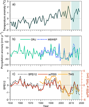
Figure 1. Inter-annual variation in (a) annual temperature anomaly, (b) annual precipitation anomaly from CRU (green) and MSWEP (blue), and (c) mean annual SPEI12 (black), scPDSI (red) and TWS (yellow). The vertical yellow and blue shading area mark the severe drought (2000–2009) and post-drought (2010–2018) periods, respectively. See text for details.
Download figure:
Standard image High-resolution image3.2. Vegetation productivity during and after drought
During the severe 10 year drought,  was 15% lower than after drought (2000–2009 vs. 2010–2018). Also during the severe 10 year drought (2000–2009),
  was 8.9% lower than during the post-drought period 2010–2018. Indeed, we found an overall significant positive relationship between
  and
and  (R2 = 0.53, p < 0.001), which was significant in 78.0% of the grid cells (78.5% and 77.1% in MN and IM, respectively) (figure S5(a)). The lowest
  of the study period occurred in 2007, consistent with a persistent decrease in scPDSI and SPEI until 2007. Then,
  started to recover from the severe drought with increasing
  beginning in 2008, but the
  anomaly remained negative until 2010. The increase in
  by 0.06 between the periods 2010–2018 and 2000–2009 was mainly attributed to increased
  during the summer (
 ; 68.2%) and spring (
 ; 19.3%) (table 1). Summer still plays the leading role when focusing on the sub-region scale, and the contribution proportions are 76% and 61% for MN and IM, respectively (table S2). The spatial pattern of
  recovery shows that summer is the dominant season driving recovery in 83.5% grid cells (85.0% and 81.3% in MN and IM, respectively) (figure S4(c)). As the correlation results show, summer precipitation was the dominant factor determining
  , and
, and  explained more of the residual variation (64%) than
  (45%) and
  (21%) (table 2). The partial correlation coefficient between
  and
and  was significant when controlling for the effects of summer precipitation and temperature for MP and IM (p < 0.05).
Table 1. Seasonal contribution to the change in the mean integrated growing season NIRV between two periods (2000–2009, 2010–2018). Growing season:  ; spring:
  ; summer:
  ; autumn:
  .
.
| Integrated NIRV (2000–2009) | Integrated NIRV (2010–2018) | Difference in integrated NIRV between 2010–2018 and 2000–2009 | Contribution (%) | |
|---|---|---|---|---|

| 0.62 | 0.67 | 0.06 | 100.00 |

| 0.12 | 0.13 | 0.01 | 19.32 |

| 0.37 | 0.41 | 0.04 | 68.15 |

| 0.13 | 0.13 | 0.01 | 12.53 |
Table 2. Correlation coefficients between seasonal integrated  (
( ,
, ,
,  ,
, ) and related variables during 2000–2018. P = total precipitation. SM0 = soil moisture of the month preceding the season, i.e. March for spring, May for summer, August for autumn, and March for growing season. SM = mean soil moisture. T = temperature . The value in parenthesis = the correlation coefficient between
  and total precipitation in June and July. * and ** indicated relationships that are significant at the level p < 0.05 and p < 0.01, respectively.
| P | SM0 | SM | T | |
|---|---|---|---|---|
| NIRV AM | 0.25 | 0.75** | 0.88** | 0.07 |
| NIRV JJA | 0.67** (0.80**) | 0.46 | 0.85** | −0.36 |
| NIRV SO | 0.18 | 0.34 | 0.34 | 0.25 |
| NIRV GS | 0.73** | 0.46 | 0.86** | −0.30 |
3.3. Effect of pre-growing season soil water storage
Despite the overall strong relationship between precipitation and vegetation productivity, some years with similar  (220–240 mm) had very different levels of vegetation productivity (~50% of total 2000–2018 range). For example, in 2003, despite high
  (42.7 mm above the 2000–2018 average, figure 2(b)), the anomaly of vegetation productivity was negative ('anomaly' in the study refers to the deviation from the mean). A comparison between 2007 and 2017, which had similarly low
  (209 mm and 219 mm, respectively), provides an example of the mismatch of NIRv and P. Spring precipitation (
 ) in 2017 was 32% lower than that in 2007, but
  in 2017 was 12% higher than in 2007. This higher
  despite lower spring precipitation in 2017 is related with the higher SM and TWS in March of 2017 (figures 3(c) and (d), table S3). The positive SM anomaly in 2017 lasted from March to June, alleviating the
  deficit in 2017 (figure 3(d)). On the other hand, the negative
  anomaly in 2007, propagated from the depleted soil water in the previous consecutive drought years (2000–2006), contributed to low
  in 2007. The TWS anomaly in 2007 from reconstructed GRACE data also showed a deficit of water storage in March, resulting from the previous drought years. Furthermore, as the correlation results show (table 2; Table S4), the soil moisture in March (
 ) is highly correlated with spring
  (
( ) for all three regions (MP, MN and IM; p < 0.05). The partial correlation between
  and
and  is significant for MP and IM (p < 0.05) after controlling for the effect of GS precipitation and temperature. Furthermore,
  explained 35% and 29% of the residual variation in
  , predicted from
  for MP and IM, respectively (figure 2(f)). This relationship was significant over 20% and 28% of regional grids for MP and IM, respectively (figure S5(b)). For MN, the partial correlation between
  and
and  are only marginally significant (R = 0.47; p = 0.06) driven by a weaker relationship between spring
  and GS
  (R = 0.43, p = 0.06).

Figure 2. Temporal variation of (a) integrated NIRV anomaly, (b) precipitation anomaly, and (c) soil moisture anomaly, from 2000–2018 and (d) maximum SWE anomaly from 2000 to 2016. Growing season anomaly (circle), spring anomaly (orange), summer anomaly (red), and autumn anomaly (grey) are shown. (e) Relationship between growing season precipitation ( ) and
) and  from 2000 to 2018. (f) Relationship between soil moisture in March (
 ) and the residual of
  predicted by
  from 2000 to 2018.
Download figure:
Standard image High-resolution image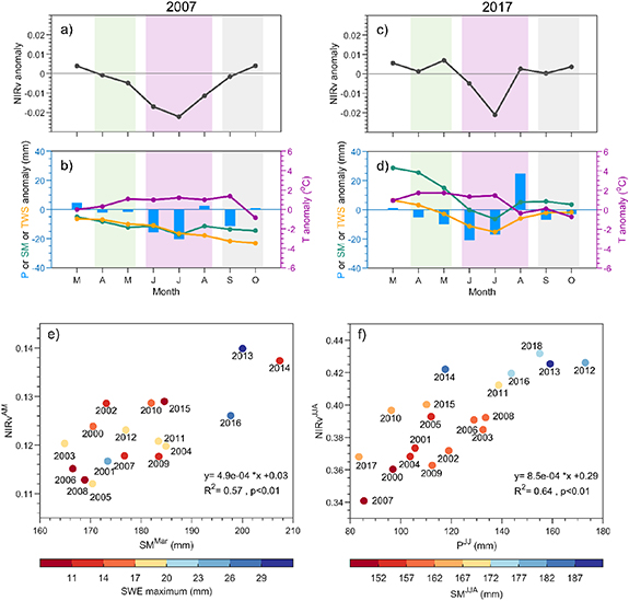
Figure 3. Anomaly of monthly (a) and (c) NIRv, (b) and (d) precipitation (blue bars), soil moisture (green lines), TWS (yellow lines) and temperature (purple lines) in 2007 (a) and (b) and 2017 (c) and (d), relative to the period 2000–2018. (e) Relationship between soil moisture in March ( ) and integrated spring NIRV (
 ) from 2000 to 2016. The colors indicate the maximum snow water equivalent (SWE) of the previous winter. (f) Relationship between precipitation in June and July (
 ) and integrated summer NIRV (
 ). The colors indicate summer soil moisture (
 ).
).
Download figure:
Standard image High-resolution imageSoil moisture in the previous Octoberx ( is highly correlated with
  for all three regions (p < 0.001). The
  was 12%, 11%, and 13% higher in 2010–2018 than in 2000–2009 for MP, MN, and IM, respectively. For IM, there is a direct and significant correlation between maximum SWE and
  (p < 0.05), and the correlation is stronger after controlling for the effect of
  (p < 0.01). For MN, though there is not a significant correlation between SWE and
  , SWE is significantly correlated with the difference between
  and
and  (p = 0.02), and the relationship is stronger when controlling for the
  (p = 0.01).
3.4. Change in livestock number and its relationship with vegetation productivity
In MN, livestock numbers dropped in 2000–2002 (figure 4(a)), following severe drought onset in 2000 (figure 1(c)). The drop ended a persistent increase since the 1970s (except for camel). From 2000 to 2002, the total livestock number declined by 37% relative to 1999. These declines were 51% for cattle, 37% for horse, 30% for sheep, 29% for camel, and 17% for goat. Since 2003, the population of the three most commonly reared livestock types, sheep, goat, and cattle, has increased slowly, while horse and camel population numbers remain relatively unchanged. By 2009, the number of sheep and goats exceeded that before the severe drought, but camel, horse and cattle numbers were below pre-drought level. As vegetation productivity recovered from drought during 2010–2018, the total livestock number increased at a rate twice that in 2002–2009 (figure 4(a)). The change in livestock number was closely linked to vegetation productivity in MN. The detrended livestock number was significantly correlated with the detrended 3 year moving average  in most aimags in central and eastern MN (figure 4(b)). The livestock populations in these regions make up 55% of the total national livestock units. Furthermore, the relationship between livestock number and vegetation productivity was strongest in the areas with the most livestock (figure 4(c)).
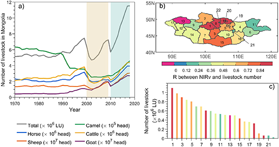
Figure 4. (a) Interannual variations of livestock numbers from 1970 to 2018 in Mongolia (total-grey; horses-blue; sheep-orange; camel-green; cattle-yellow; goat-purple). 'LU' = 'livestock unit'. (b) Spatial pattern of correlation coefficient (R) between yearly livestock number and  (3 year moving average) by aimag. (c) Livestock number in 2018 in each aimag. Numbers (1–22) are the aimag IDs, sorted according to their livestock number in 2018 (from large to small).
Download figure:
Standard image High-resolution imageThe temporal pattern of  in IM was similar to the pattern in MN (R = 0.77, p < 0.001, figure S7). However, the severe decadal drought in the early 2000s had relatively less impact on livestock numbers in IM (figure 5). Total livestock number decreased in the early years of the drought (2000 and 2001), but increased by 45% from 1999 to 2010. As a result, the detrended total livestock number was negatively correlated with the detrended 3 year moving average
  (R = −0.45, p = 0.08).
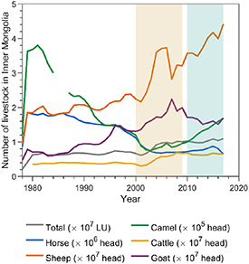
Figure 5. Interannual variations of livestock numbers by type from 1978 to 2017 in Inner Mongolia. 'LU' = 'livestock unit'.
Download figure:
Standard image High-resolution image4. Discussion
4.1. Recovery of vegetation productivity from the severe decadal drought
Evaluated with scPDSI (SPEI), the severe decadal drought reached its worst point in 2007. It still remained below −2 (−1) in 2008–2009, suggesting the continuation of the drought. This unprecedented long-term drought caused a significant decrease in pasture productivity and damaged the livestock sector (Nandintsetseg and Shinoda 2013), and also caused this region to shift from a carbon sink to a carbon source (Lu et al
2019). Starting in 2010, the drought indices rebounded, and the  anomaly changed to positive while
  returned to its 1982–2016 average level (figure S6). Although vegetation productivity was still suppressed by drought in 2008 and 2009, soil water started to recover, which contributed to vegetation recovery since 2010 (figure 2(d)). The 2 or 3 years required for recovery of grassland vegetation productivity after this severe drought is generally shorter than what would be expected of forests, due to the different hydraulic traits, water use strategies and growth rate of herbaceous- vs. woody-plant dominated ecosystems (Anderegg et al
2019, Schwalm et al
2017, Kolus et al
2019).
returned to its 1982–2016 average level (figure S6). Although vegetation productivity was still suppressed by drought in 2008 and 2009, soil water started to recover, which contributed to vegetation recovery since 2010 (figure 2(d)). The 2 or 3 years required for recovery of grassland vegetation productivity after this severe drought is generally shorter than what would be expected of forests, due to the different hydraulic traits, water use strategies and growth rate of herbaceous- vs. woody-plant dominated ecosystems (Anderegg et al
2019, Schwalm et al
2017, Kolus et al
2019).
Several previous studies have demonstrated the importance of post-drought precipitation for recovery of productivity (Antofie et al
2015, Schwalm et al
2017, He et al
2018), which is also evident in our study. In the MP, most of the precipitation occurs in summer (64%, 63%, and 66% for MP, MN and IM, respectively). Interestingly, summer was also the season with the most precipitation increase between 2000–2009 and 2010–2018 (61%, 65%, and 58% of the annual precipitation increase for MP, MN and IM, respectively). As a result, the strong correlation between  and
and  played a determined role for the increase in summer vegetation productivity between the two periods. However, the effect of spring precipitation on the vegetation productivity should not be overshadowed. For example, in the two transitional years, 2009 and 2010, though rainfall only increased during the spring (27 mm) and autumn (11 mm) and actually decreased in the summer (−11 mm) of 2010 compared with 2009,
  of the three seasons was higher in 2010 than in 2009 (figure 2). Since the
  is similar in 2 years (183, 182 mm), it is the increase in spring precipitation that enhanced grassland productivity in spring and summer. The spring precipitation exerts its influence on vegetation productivity in three aspects: (a) promoting spring productivity, (b) leaving water for plants to use in summer, which can be seen from the significant partial correlation between
  and
and  (after removing the effect of
  ) as well as the significant partial correlation between
  and
and  , (c) enabling plants to expand the leaves to better photosynthesize and develop the root system to fully utilize the available water during the late months (Bates et al
2006, Peng et al
2013). Thus, in this region spring rainfall may be more critical for post-drought vegetation productivity recovery than the same amount of rainfall in summer or autumn.
, (c) enabling plants to expand the leaves to better photosynthesize and develop the root system to fully utilize the available water during the late months (Bates et al
2006, Peng et al
2013). Thus, in this region spring rainfall may be more critical for post-drought vegetation productivity recovery than the same amount of rainfall in summer or autumn.
4.2. Effect of pre-growing season soil water storage
Our results suggest that pre-GS SM plays a key role in spring grassland vegetation productivity. For example, by comparing 2007 and 2017, we showed that a deficit of water storage in March resulting from the previous drought years could amplify the drought effect of deficit of  on vegetation productivity in 2007; while a positive pre-GS SM anomaly helped alleviate the drought impact in 2017 and led to higher
  . Higher pre-GS SM advances leaf-out phenology of grasslands (Shen et al
2011, Ganjurjav et al
2016) and provides effective moisture for spring growth (Shen et al
2011, Wang et al
2018). Both higher residual SM from previous GS and higher winter snowfall resulted in higher
. Higher pre-GS SM advances leaf-out phenology of grasslands (Shen et al
2011, Ganjurjav et al
2016) and provides effective moisture for spring growth (Shen et al
2011, Wang et al
2018). Both higher residual SM from previous GS and higher winter snowfall resulted in higher  in 2011–2013, compensating for the spring precipitation deficits (figures 2(b) and (d)). In contrast, long-term drought in the 2000s exacerbated the deficit of
  by amplifying the deficit of residual SM from the previous GS (figure 2(c)). Snowfall, an important moisture source, could help vegetation resist drought in arid and semi‐arid regions (Peng et al
2010, Li et al
2020). In IM, because of warmer early spring temperatures, the snow has melted and permeated into the soil by March, reflected by the significant correlation between SWE and
by amplifying the deficit of residual SM from the previous GS (figure 2(c)). Snowfall, an important moisture source, could help vegetation resist drought in arid and semi‐arid regions (Peng et al
2010, Li et al
2020). In IM, because of warmer early spring temperatures, the snow has melted and permeated into the soil by March, reflected by the significant correlation between SWE and  , promoting vegetation productivity in April (significant correlation between SWE and
  ). In contrast, in MN, the melting process starts later and can lag into April, reflected by the significant correlation between SWE and the difference in SM between March and April. In addition to the benefits of snow as a water source for vegetation, deep snow is also an effective insulator, inhibits wind soil erosion, and increases nutrient availability by enhancing soil temperature and facilitating microbial activity and mineralization (Schimel et al
2004, Schmidt and Lipson 2004, Tomaszewska et al
2020).
). In contrast, in MN, the melting process starts later and can lag into April, reflected by the significant correlation between SWE and the difference in SM between March and April. In addition to the benefits of snow as a water source for vegetation, deep snow is also an effective insulator, inhibits wind soil erosion, and increases nutrient availability by enhancing soil temperature and facilitating microbial activity and mineralization (Schimel et al
2004, Schmidt and Lipson 2004, Tomaszewska et al
2020).
Using stable isotopes of hydrogen and oxygen at one grassland site in IM, Chi et al (2019) demonstrated that contribution of snow to plant water uptake continues throughout the whole GS. However, in our study, the significant correlation between  (
( for MN) and the monthly
  ends in June. We thus infer that the legacy of snow water lasts no later than June in our study. This shorter legacy period could be because the regional mean SWE is in the range of 5–40 mm in this study, while the maximum SWE was ~159 mm in the snow-addition plot in Chi et al (2019). The difference in snow depth between the two studies indicates that the legacy time of snow water uptake depends on the amount of SWE. By conducting isotope observation at one grassland site in Tibetan Plateau, Hu et al (2013) claimed that once the monsoon season starts, plants tend to use topsoil moisture mainly from rainfall rather than residual moisture from snow (Hu et al
2013). How long the legacy effect of snow water for vegetation growth can last in the GS is not well known yet, and it is relevant to local climate and water partition between species (Yang et al
2011, Trnka et al
2015, Potopová et al
2016). Hence, further observation, manipulative experiments and modeling are needed.
ends in June. We thus infer that the legacy of snow water lasts no later than June in our study. This shorter legacy period could be because the regional mean SWE is in the range of 5–40 mm in this study, while the maximum SWE was ~159 mm in the snow-addition plot in Chi et al (2019). The difference in snow depth between the two studies indicates that the legacy time of snow water uptake depends on the amount of SWE. By conducting isotope observation at one grassland site in Tibetan Plateau, Hu et al (2013) claimed that once the monsoon season starts, plants tend to use topsoil moisture mainly from rainfall rather than residual moisture from snow (Hu et al
2013). How long the legacy effect of snow water for vegetation growth can last in the GS is not well known yet, and it is relevant to local climate and water partition between species (Yang et al
2011, Trnka et al
2015, Potopová et al
2016). Hence, further observation, manipulative experiments and modeling are needed.
4.3. Mitigation of drought impacts on livestock
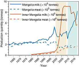
Drought-caused changes in grassland vegetation productivity can impact the stock number of cattle, sheep, and goats (Nardone et al 2010, O'Mara 2012). The impact of drought on livestock is particularly clear for MN (figure 4). During the severe decadal drought in the 2000s, livestock number in MN decreased (figure 4), and milk and meat production declined by 42% and 40% from 1999 (figure 6). The livelihoods of herders were threatened and some were forced to give up herding completely due to economic losses during the severe decadal drought (Rao et al 2015). In contrast, the number of livestock and livestock products increased during the 2000s in IM (figures 5 and 6). The increase may be attributed to increased forage import and crop residues compensating the shortage of grass feed during the drought (National Bureau of Statistics of China 2019). Although the short-term droughts in the 2010s had smaller impacts than the long-term drought in the 2000s on the livestock sector in MN, more effective mitigation measures and policies will be required for the livestock sector in MN to survive the predicted future drying trend in MP (Chen et al 2015, 2018, Hessl et al 2018). The different responses to droughts between MN and IM shown in this study could offer important insights for future drought mitigation (Chen et al 2015). In addition, climate change could lead to more harsh winters (Cohen et al 2014), which increase livestock mortality (Fernandez-Gimenez et al 2015). The ultimate impacts of the trade-off between the benefit of snow water for vegetation growth and the damage of harsh winters on livestock remains uncertain and needs further investigation.
Figure 6. Interannual variations of livestock product quantity in Mongolia (blue lines) between 1961 and 2018 and Inner Mongolia (red lines) between 1980 and 2018.
Download figure:
Standard image High-resolution image
5. Implications and conclusions
During a severe decadal drought from 2000 to 2009 on MP, soil water deficit reached its maximum, and vegetation productivity was lowest, in 2007. However, by 2010, drought conditions were alleviated and vegetation productivity returned to the long-term mean value. Short-term droughts also occurred in this region in the 2010s, with less reduction in vegetation productivity compared to the decadal drought in the 2000s. Our findings highlight the critical role of early GS precipitation and winter/spring snowfall in determining the extent to which vegetation productivity declines in response to drought. We focused on total vegetation productivity here, but it is possible that drought could cause a change in plant community composition (Knapp et al 2020, Li et al 2020), which could alter the sensitivity of grasslands productivity to precipitation. Whether a shift in plant community composition would increase or decrease the sensitivity of vegetation productivity to precipitation in this region is still an open question warranting further investigation. Though MP is unlikely to experience another severe decade drought in this century (Hessl et al 2018), climate models for the region predict a drying trend until the middle of this century as well as potential changes in the seasonal pattern of precipitation (IPCC 2013, Groisman et al 2018). Our findings will be particularly useful for understanding the impacts of predicted shifts in precipitation seasonality. Exploring the vegetation response to different durations of drought and different precipitation patterns will provide critical information to support policy decisions and livestock management in this arid and semi-arid region.
Acknowledgments
This study was supported by the National Key Research and Development Program of China (Grant Number 2016YFC0500203), and the National Natural Science Foundation of China (Grant Numbers 41722101, 41671079). We thank Melinda D. Smith for her comments and suggestions.
Data availability statement
The data used in this study can be publicly accessed. MODIS NIRT and NDVI data are available from https://lpdaac.usgs.gov/products/mod13a2v006/. The GIMMS NDVI data is available from https://ecocast.arc.nasa.gov/data/pub/gimms/3g.v1/. The MCD12Q1 land cover data can be downloaded from https://lpdaac.usgs.gov/products/mcd12q1v006/. The CRU TS v4.03 climate data sets are available from CRU (https://crudata.uea.acuk/cru/data/hrg/cru_ts_4.03/). The MSWEP precipitation dataset can be accessed on website http://gloh2o.org/. The SM data from GLEAM can be accessed from https://www.gleam.eu/. The snow water equivalent (SWE) from GlobSnow is available from www.globsnow.info/swe/archive_v2.0/. The TWS can be downloaded from https://figshare.com/articles/GRACE-REC_A_reconstruction_of_climatedriven_water_storage_changes_over_the_last_century/7670849. The livestock number data for MN is from the National Statistical Office of Mongolia website (www.en.nso.mn/). The livestock product data for Mongolia is from FAO (http://www.fao.org/faostat/en/#data/QL). The livestock number and product data for IM of China is from National Bureau of Statistics of China website (http://data.stats.gov.cn/). The drought index scPDSI can be accessed from https://crudata.uea.acuk/cru/data/drought/. The drought index SPEI can be accessed from https://spei.csic.es/database.html.
All data that support the findings of this study are included within the article (and any supplementary files).