


1. Introduction
Boundary layer instability over a rotating body of revolution (disk, cone, sphere, etc.) is an intriguing problem in fluid mechanics. Such instability is encountered at different scales, ranging from small-scale phenomena in laboratory experiments to large-scale atmospheric events. Generally, when the boundary layer over a rotating solid body becomes unstable, perturbations in the flow field can amplify and induce coherent flow structures (Kobayashi Reference Kobayashi1994). The mechanisms causing such boundary layer instability depend on the geometry and flow conditions. When investigating such three-dimensional boundary layer instability mechanisms over a rotating body, the case of a rotating cone is usually preferred, since the relatively simple geometry eases the analysis (Kobayashi, Kohama & Kurosawa Reference Kobayashi, Kohama and Kurosawa1983; Kohama Reference Kohama1984a). Additionally, a rotating cone is often considered as an idealised model of engineering systems, such as aero engine spinners, the nose cones of rotating projectiles (missiles, bullets), etc. Several past studies have contributed to building our understanding of the boundary layer instability over a rotating cone, but they are limited to an axisymmetric inflow field. While symmetry about the axis simplifies the analysis, in practice, deviations from a perfectly symmetric inflow may frequently occur due to off-design conditions or sometimes as consequences of design choices, e.g. embedded engines ingesting the airframe boundary layer, ultra-high-bypass-ratio engines with short intakes at take-off and cross-wind operations, etc. Therefore, it is important to extend our understanding of the boundary layer instability over a rotating cone to the non-axial (thereby non-axisymmetric) inflow.
In the past, the boundary layer instability mechanism over a rotating slender cone with half-angle  $\psi =15^\circ$ has been studied in still fluid (Kobayashi & Izumi Reference Kobayashi and Izumi1983) as well as under axial inflow (Kobayashi et al. Reference Kobayashi, Kohama and Kurosawa1983). The boundary layer on the rotating surface faces centripetal acceleration, which may lead to an instability, commonly known as centrifugal instability. Depending upon the rotational speed, toroidal vortices form over a cone rotating in still fluid (Kobayashi & Izumi Reference Kobayashi and Izumi1983), whereas spiral vortices appear on a rotating cone under an enforced axial inflow (Kobayashi et al. Reference Kobayashi, Kohama and Kurosawa1983). In meridional cross-sections, these vortices appear as consecutive pairs of counter-rotating vortices. Their azimuthal number
  $n$ and angle
  $\phi$ depend on the local rotational speed ratio
  $S=r\omega /u_e$, where
  $r$ is the local radius,
  $\omega$ is the angular velocity of the cone and
  $u_e$ is the local boundary layer edge velocity. With increasing local rotational speed ratio
  $S$ (from
  $S=0$ to 5–6), both
  $n$ and
  $\phi$ decrease as the spiral structure of the vortices starts to approach a toroidal structure. Between
  $S\approx 6$ and
  $8$, the vortex structure becomes toroidal, similar to that observed over a rotating cone in still fluid (Kobayashi & Kohama Reference Kobayashi and Kohama1985). However, the scope of the present study is limited to rotational speed ratios
  $0<S<5$, and, therefore, the rest of the discussion is focused on spiral vortices.
Kohama (Reference Kohama1984a) studied the behaviour, growth and breakdown of spiral vortices using particle-based flow visualisation. While tracking the growth of spiral vortices, Kohama observed that the wall-normal extent of these vortices increased beyond the boundary layer thickness. In this region, the mixing of low- and high-momentum fluid is enhanced, forming shear layers of different scales. Kohama (Reference Kohama1984a) suggested that this enhanced activity of mixing affects the mean velocity profiles and could be the leading cause of boundary layer transitioning to a fully turbulent state. Recently, Hussain et al. (Reference Hussain, Garrett, Stephen and Griffiths2016) revisited this topic and developed a distinct theoretical analysis based on the centrifugal instability mode. They highlighted that, even though cross-flow and Tollmien–Schlichting instabilities are present in the flow field, the centrifugal instability is prevalent. Garrett & Peake (Reference Garrett and Peake2007) and Garrett, Hussain & Stephen (Reference Garrett, Hussain and Stephen2009) also state that, for a rotating slender cone (half-angle  $\psi <40^\circ$), the cross-flow and absolute instabilities may not play a dominant role in the boundary layer transition. Kobayashi (Reference Kobayashi1994) found that spiral vortices, in the form of counter-rotating vortex pairs, appear over a rotating cone with half-angle
  $\psi <30^\circ$; whereas for a rotating cone with
  $\psi >30^\circ$, co-rotating spiral vortices are observed. Theoretical studies performed by Garrett, Hussain & Stephen (Reference Garrett, Hussain and Stephen2010) show that the cross-flow instability mode is dominant on rotating broad cones (half-angle
  $\psi >40^\circ$) in axial inflow. In such cases, with increasing local radius, the increasing tangential velocity of the rotating cone surface leads to a streamwise pressure gradient along the cone length. This pressure gradient results in an inflectional profile of the mean streamwise velocity that leads to cross-flow instability (Kohama Reference Kohama1984b; Garrett et al. Reference Garrett, Hussain and Stephen2010). Recent experiments by Kato, Alfredsson & Lingwood (Reference Kato, Alfredsson and Lingwood2019a) and Kato et al. (Reference Kato, Kawata, Alfredsson and Lingwood2019b) also show the existence of co-rotating spiral vortices (relating to the cross-flow instability) over a broad cone (
 $\psi =60^\circ$) rotating in still fluid. Overall, past research provides detailed insights into the formation, growth and breakdown of spiral vortices over a rotating cone, but all of these detailed studies are limited to axisymmetric inflow conditions.
Depending on the inflow conditions and cone angle, both centrifugal and cross-flow instability mechanisms lead to spiral vortices over a rotating cone. Generally, vortices generated by the centrifugal instability are of counter-rotating nature in their cross-sections. This behaviour has also been observed in flow cases other than rotating cones, where the centrifugal instability is present, e.g. Görtler vortices on concave walls (Görtler Reference Görtler1954; Drazin Reference Drazin2002), Taylor vortices between two rotating coaxial cylinders (Taylor Reference Taylor1923; Drazin Reference Drazin2002), etc. Recent studies have shown the existence of the centrifugal instability mode over a spinning cylinder in uniform flow, orthogonal to the rotation axis (Mittal Reference Mittal2004; Radi et al. Reference Radi, Thompson, Rao, Hourigan and Sheridan2013; Rao et al. Reference Rao, Leontini, Thompson and Hourigan2013a,Reference Rao, Leontini, Thompson and Houriganb), and the vorticity contours associated with this mode suggest the counter-rotating nature of the vortices, which appear as travelling waves (Rao et al. Reference Rao, Leontini, Thompson and Hourigan2013a). On the other hand, the cross-flow instability gives rise to co-rotating vortices (Kobayashi Reference Kobayashi1994). This behaviour also extends beyond the case of a rotating cone, e.g. spiral vortices on a rotating disk (Kobayashi, Kohama & Takamadate Reference Kobayashi, Kohama and Takamadate1980; Kohama Reference Kohama1984b), cross-flow vortices over a swept wing (Kohama Reference Kohama1987), etc. Therefore, an observed vortex cross-section can be linked to a type of instability.
Considering the geometry and the associated instability mechanism, cones can be classified into two categories: slender cones (half-angle $\psi \lesssim 30^\circ$), where the centrifugal instability is dominant, and broad cones (half-angle
  $\psi \gtrsim 30^\circ$), where the cross-flow instability is dominant. The centrifugal instability over a slender cone, with half-angle
  $\psi =15^\circ$, rotating in an axisymmetric inflow field has been well addressed in the literature(Kobayashi et al. Reference Kobayashi, Kohama and Kurosawa1983, Reference Kobayashi, Kohama, Arai and Ukaku1987; Kohama Reference Kohama1984a). Therefore, the present study is focused on this geometry to investigate the effect of non-axial inflow on the centrifugal instability.
The present study shows how a deviation from a symmetric inflow condition affects the development of spiral vortices, induced by the centrifugal instability, over a rotating slender cone with half-angle  $\psi =15^\circ$. The definitions of the cone geometry and flow parameters are described in § 2. The specifications of the experimental set-up and data processing methods are detailed in § 3. The detailed results and discussions are presented in § 4. The measurement approach has been validated by revisiting the axial inflow case, discussed in § 4.1. The effect of non-axial inflow on the spiral vortex appearance and growth is discussed in § 4.2. A physical interpretation of the observed differences between axial and non-axial inflow cases is presented in § 4.3. Finally, the important conclusions are discussed in § 5.
2. Definitions of geometry and flow parameters
A schematic of a rotating cone in the Cartesian coordinate system is shown in figure 1. The angular velocity  $\omega$ is aligned with the positive
  $x$ axis. The coordinate system
  $x', y'$ is used when discussing the velocities in the wall-parallel and wall-normal directions, respectively. The cone surface is represented by
  $l$ and
  $\theta$, based on cylindrical polar coordinates. Here,
  $l$ is the meridional distance from the cone apex, and
  $\theta$ is the azimuthal angle measured from the counter-rotating meridian.
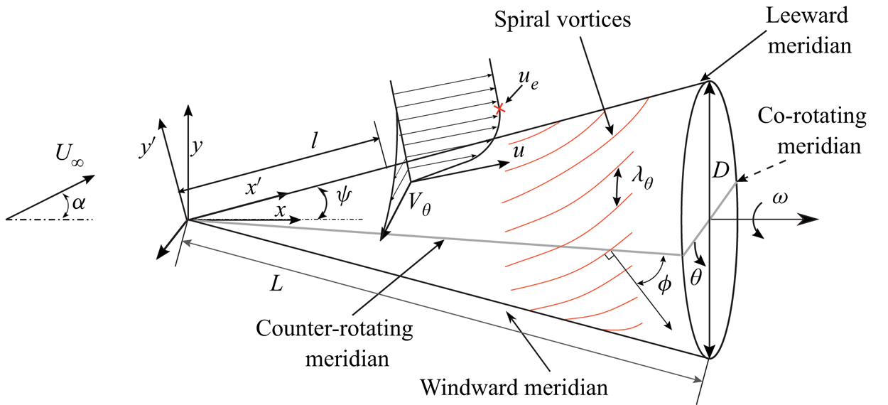
Figure 1. Schematic of the rotating cone and coordinate systems.
The local Reynolds number  $Re_l$ and local rotational speed ratio
  $S$ are the important flow parameters that govern the spiral vortex growth (Kobayashi et al. Reference Kobayashi, Kohama and Kurosawa1983, Reference Kobayashi, Kohama, Arai and Ukaku1987). Their definitions are as follows:
 \begin{equation} Re_l=\frac{u_e l}{\nu}, \quad S=\frac{r\omega}{u_e}. \end{equation}
Here,  $u_e$ is the boundary layer edge velocity,
  $\nu$ is the kinematic viscosity of air,
  $r$ is the local radius and
  $\omega$ is the angular velocity of the cone.
The boundary layer edge velocity  $u_e$ is defined as the time-averaged streamwise velocity, measured at a wall-normal location where the magnitude of the vorticity component out of the meridional plane reaches zero. In practice, the vorticity is considered to be zero below the value of measurement uncertainty (
 ${<}0.24U_\infty /D$), where
  $U_{\infty }$ is the free-stream velocity and
  $D$ is the base diameter of the cone. For the axial inflow, the boundary layer edge velocity over the entire cone is obtained by fitting a power-law form
  $u_e=CU_{\infty }l^m$ (Garret & Peake Reference Garrett and Peake2007) to the measured velocity field for
  $l/D=0.8$ to
  $1.8$ (
 $C=1.66$,
  $m=0.19$ and root-mean-square (r.m.s.) fit error
  $< 0.02 U_{\infty }$).
Although the spiral vortex growth depends on the local scaling  $S$ and
  $Re_l$ (Kobayashi et al. Reference Kobayashi, Kohama, Arai and Ukaku1987), the inflow Reynolds number
  $Re_L$ and the base rotational speed ratio
  $S_b$ are useful parameters while discussing the experimental conditions. They are defined as follows:
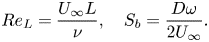 \begin{equation} Re_L=\frac{U_\infty L}{\nu}, \quad S_b=\frac{D\omega}{2U_\infty}. \end{equation}
Here,  $L=D/(2\sin (\psi ))$ is the total cone length along
  $x'$, and a subscript
  $b$ refers to the cone base. The dependence on the finiteness of a cone can be eliminated by defining a parameter
  $\kappa$ as
 \begin{equation} \kappa=\frac{Re_L}{S_b}=\frac{U_{\infty}^2}{\sin(\psi) \omega \nu}. \end{equation}
Here,  $\kappa$ depends only on the cone half-angle, angular velocity and free-stream conditions. Since
  $\kappa$ is the slope of the line
  $Re_L=\kappa S_b$, it provides a general direction along which the curves of
  $Re_l$ versus
  $S$ lie for particular experimental conditions. In the subsequent text,
  $S_b$,
  $Re_L$ and
  $\kappa$ are used while referring to different inflow conditions and, consequently, for the different distributions of local flow parameters
  $Re_l$ and
  $S$ over the cone.
Figure 1 also schematically shows the spiral vortices and their characteristics. Here, the spiral vortex angle  $\phi$ is the angle between the meridional line and the direction of the perturbation wave propagation; this is same as the angle between the vortex axis direction and the circumferential direction (Kobayashi et al. Reference Kobayashi, Kohama and Kurosawa1983). The azimuthal number of vortices
  $n$ ideally represents the azimuthal wavelength
  $\lambda _\theta =2{\rm \pi} r/n$.
3. Experimental set-up
The experiments are performed in a low-speed open jet wind tunnel facility (named  $W$ tunnel) at the Faculty of Aerospace Engineering, TU Delft. The exit cross-section is
  $0.6\ \textrm {m} \times 0.6\ \textrm {m}$. A slender cone (half-angle
  $\psi =15^\circ$, base diameter
  $D = 0.047\ \textrm {m}$), made out of polyoxymethylene, is rotated by a brushless motor at
  $5000$ r.p.m. The non-axial inflow is imposed by varying the incidence angle
  $\alpha$ between
  $0^\circ$ and
  $10^\circ$. Since the present study is focused on deviations from axial symmetry, first, small variations in the incidence angles are considered (
 $\alpha =2^\circ$ and
  $4^\circ$). A considerably larger value of
  $\alpha =10^\circ$, which corresponds to a relative incidence
  $\alpha /\psi =0.67$, is also tested. High values of incidence angles may cause flow separation, and such investigations are beyond the scope of the present study. The inflow velocity of the wind tunnel is varied over
  $2.46\text {--}6.15\ \textrm {m}\ \textrm {s}^{-1}$ to obtain different values of the base rotational speed ratio
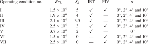
  $S_b$, and,therefore, different distributions of local Reynolds number
  $Re_l$ and rotational speed ratio
  $S$. The test matrix is presented in table 1.
Table 1. Test matrix.
It is known that coherent spiral vortices are counter-rotating in nature for cone half-angles  $\psi < 30^\circ$ (Kobayashi et al. Reference Kobayashi, Kohama and Kurosawa1983), and can be identified by their traces on the surface temperature (Tambe et al. Reference Tambe, Schrijer, Rao and Veldhuis2019). As depicted in figure 2, in the region of their mutual downwash, the local heat transfer coefficient is higher, and, therefore, the cone surface is cooled to a greater extent compared to the region of mutual upwash. When observed with infrared thermography (IRT), this results in alternating dark (cool) and bright (hot) fringes, with a vortex pair in between two consecutive bright (or dark) fringes. To increase the thermal contrast, the cone is radiatively heated with a white light source from one side (slightly increasing the model temperature by less than
  $2$ to
  $2.5$ K) and is observed with an IR camera from the opposite side (see figure 3a). The surface temperature fluctuations are obtained as digital pixel intensity fluctuations
  $I'$. The surface temperature fluctuations for the non-rotating cone were measured on the cone surface illuminated by the lamp (for
  $\alpha =0^\circ$ and
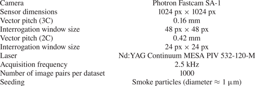
  $4^\circ$). The time-resolved velocity field is measured at the symmetry plane using particle image velocimetry (PIV) (see figure 3b). Tables 2 and 3 contain the specifications of the IRT and PIV set-ups, respectively.
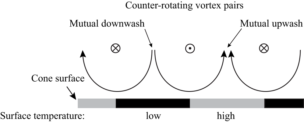
Figure 2. Surface temperature footprint of a counter-rotating vortex pair.
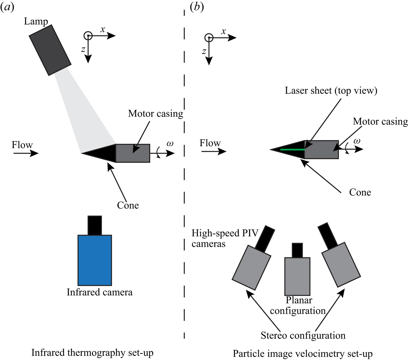
Figure 3. Schematics of the experimental set-up.
Table 2. Specifications of the infrared thermography set-up.
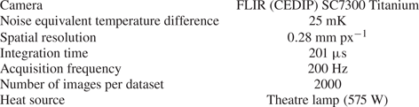
Table 3. Specifications of the PIV set-up.
In addition to the footprints of the spiral vortices, the data from IRT also include effects due to vortex pairing or free-stream disturbances. These footprints have spatial wavelengths longer than those of the spiral vortices (azimuthal vortex number  $n<8$). Additionally, the measurements also include camera noise, which appears as short spatial wavelengths (approximately
  $4$ pixels). All these effects hinder the visualisation of the spiral vortices, and are removed by following the method described in the literature (Tambe et al. Reference Tambe, Schrijer, Rao and Veldhuis2019). In this method, proper orthogonal decomposition (POD) is used to decompose the dataset as a linear combination of spatial modes with time-dependent coefficients. These spatial modes are orthogonal, and are obtained by applying singular value decomposition on the snapshot matrix of the measurement data. The traces of spiral vortices are obtained by reconstructing the temperature field using selected POD modes. The criteria for POD mode selection are defined based on the contribution of POD modes towards the expected range of streamwise wavelengths and the azimuthal number of spiral vortices. For further details on the experimental technique and data analysis method, the reader is directed to Tambe et al. (Reference Tambe, Schrijer, Rao and Veldhuis2019).
4. Results and discussion
4.1. Axial inflow
Under the axial inflow condition, spiral vortices grow in the laminar boundary layer over the rotating slender cone, leaving footprints on the surface temperature. These instantaneous footprints, which are reconstructed from the POD modes, can be seen in figures 4(a) and 4(b) as a projection in the  $xy$ plane and on an unwrapped surface, respectively (at
  $S_b=5$ and
  $Re_L=1.5 \times 10^4$). At approximately
  $x/D=0.6$, the spiral vortices start to appear in a coherent fashion, i.e. the spacing between the vortices is nearly uniform around the azimuth at a constant radius. They grow in the downstream direction until a point of maximum amplification at around
  $x/D=1.2$, beyond which their footprint deteriorates and the coherence starts to get disturbed. This growth is evident from the statistical r.m.s. of surface temperature fluctuations (
 $I'_{rms}$, computed from
  $2000$ images acquired at
  $200\ \textrm {Hz}$) shown in figures 4(c) and 4(d). Here,
  $I'_{rms}$ starts to increase around
  $x/D=0.8$, till a maximum value at around
  $x/D=1.2$, beyond which the fluctuations decrease. No such surface temperature fluctuations were observed for a non-rotating cone (
 $I'_{rms}<2$).
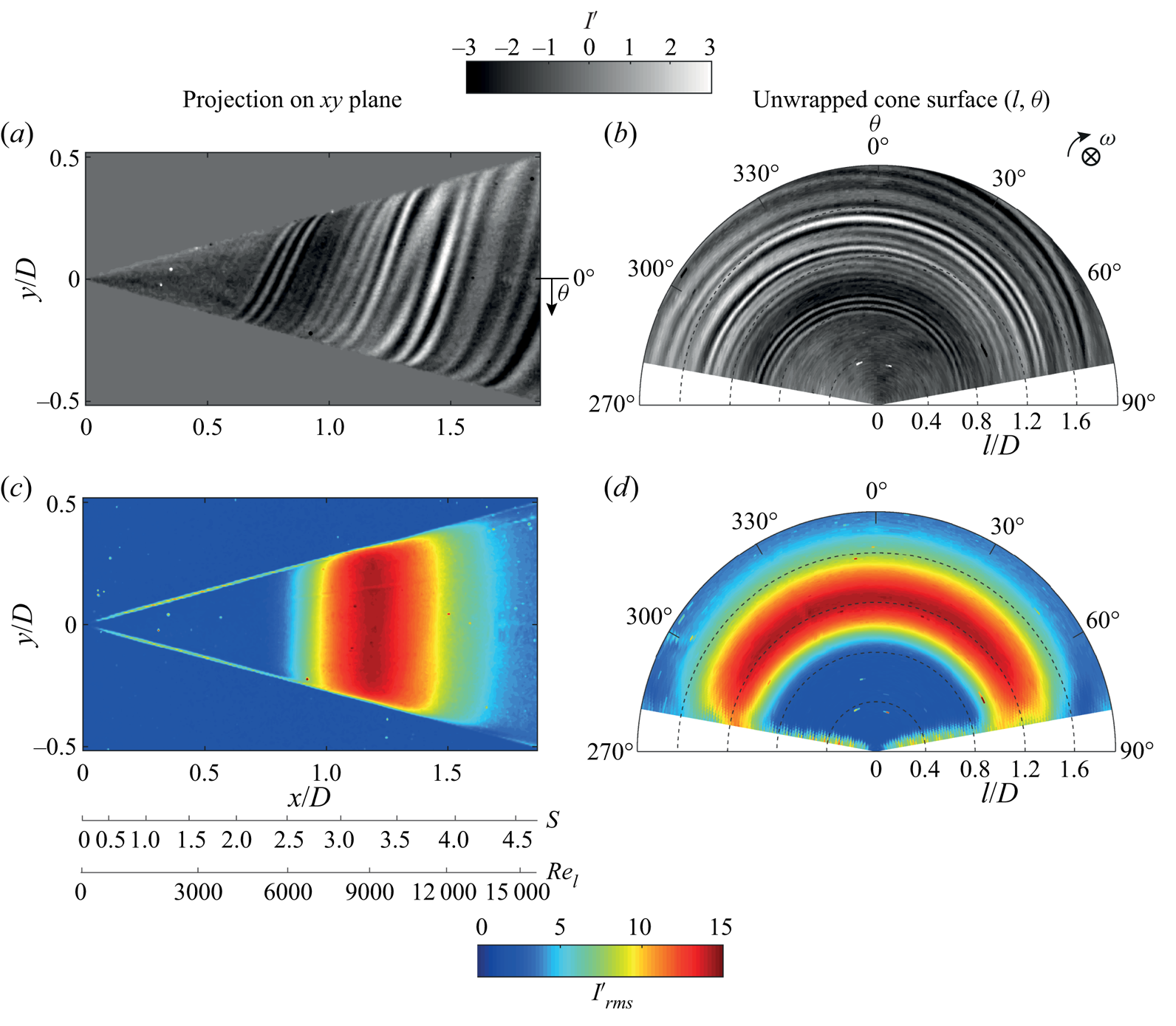
Figure 4. Instantaneous surface temperature footprints of the spiral vortices (a,b) and the corresponding statistical r.m.s. of the surface temperature fluctuations ( $I'_{rms}$) over a dataset (c,d) (here
  $\alpha =0^\circ$, operating condition I:
  $S_b=5$ and
  $Re_L=1.5 \times 10^4$).
Figure 5 allows the comparisons between (a) the meridional variation of the surface temperature fluctuations ( $I'_{rms}$ traced at
  $y/D=0$ from figures 4c), (b) the instantaneous footprints of spiral vortices over a rotating cone and their influence on (c) the mean flow field compared to (d) the mean flow of a non-rotating case. The flow phenomena occurring at the peak
  $I'_{rms}$ (point
  $l_m$ in figure 5a) can be further understood by observing the corresponding velocity fields in the wall-normal (
 $x'y'$) plane. For a non-rotating cone, the time-averaged velocity field shows a region of low streamwise momentum (along
  $x'$) close to the wall (see figure 5d). However, for the rotating cone, a similar low-momentum region is observed only until around
  $x'/D=1.24$ (see figure 5c). Beyond this point, there is a sudden increase in the
  $x'$ momentum near the wall. This point coincides with the location of the
  $I'_{rms}$ peak. It is clear that, as the spiral vortices get amplified, they transport the outer high-momentum fluid towards the wall, resulting in increased
  $x'$ momentum close to the wall. This mixing process was also observed by Kohama (Reference Kohama1984a). During the process of amplification, the local shear at the wall is increased as the outer high-momentum fluid is transported close to the wall. This increases the surface heat transfer. Consequently, the footprints of the spiral vortices become stronger in the temperature map. The maximum observed surface temperature fluctuations are of the order of
  $1.3\ \textrm {K}$. Although not shown here, a similar agreement between the location of increased
  $x'$ momentum (obtained from PIV) and the peak of
  $I'_{rms}$ (obtained from IRT) has been observed in all the investigated cases when both PIV and IRT are performed.
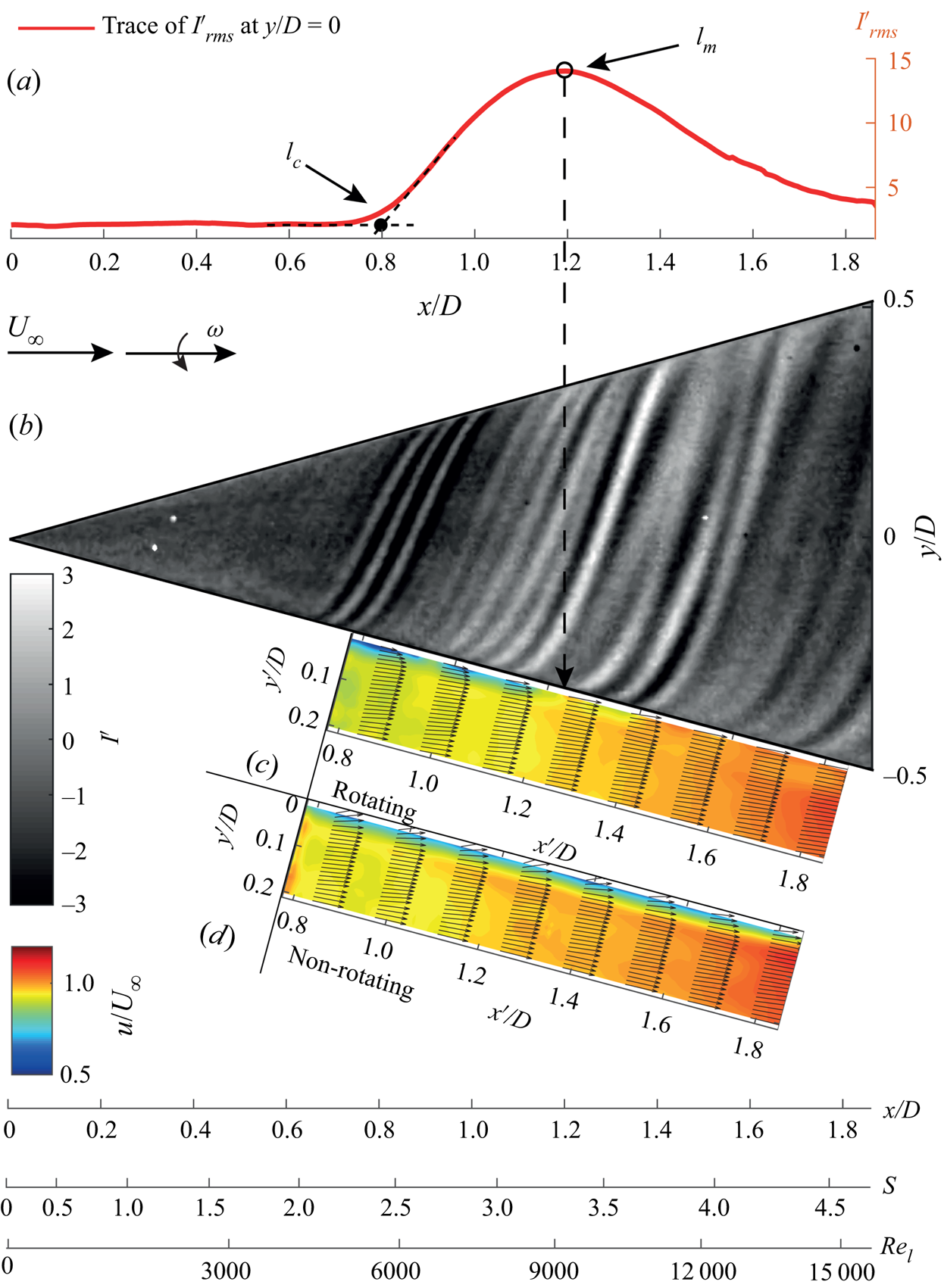
Figure 5. Growth and spatial organisation of the spiral vortices in axial inflow ( $\alpha =0^\circ$). (a) A trace of
  $I'_{rms}$ at
  $y/D=0$, (b) instantaneous surface temperature footprints of the spiral vortices over a rotating cone, and time-averaged velocity fields in
  $x'y'$ plane for (c) rotating (operating condition I:
  $S_b=5$ and
  $Re_L=1.5 \times 10^4$) as well as (d) non-rotating case (operating condition VI:
  $S_b=0$ and
  $Re_L=1.5 \times 10^4$).
Figure 6 shows the cross-sections of the spiral vortices in the symmetry plane at  $t_0+14.57T$, where
  $t_0$ is the time at the start of acquisition and
  $T=0.012\ \textrm {s}$ corresponds to the time period of a cone rotation. Additionally, supplementary movie 1 (available at https://doi.org/10.1017/jfm.2020.990) shows the time series of this vector field. The contours of wall-normal velocity fluctuations clearly show the alternating upwash and downwash regions near the wall. Together with vectors, this confirms the counter-rotating nature of the spiral vortices, which is linked to the centrifugal instability (Taylor Reference Taylor1923; Görtler Reference Görtler1954; Kobayashi et al. Reference Kobayashi, Kohama and Kurosawa1983; Rao et al. Reference Rao, Leontini, Thompson and Hourigan2013a).
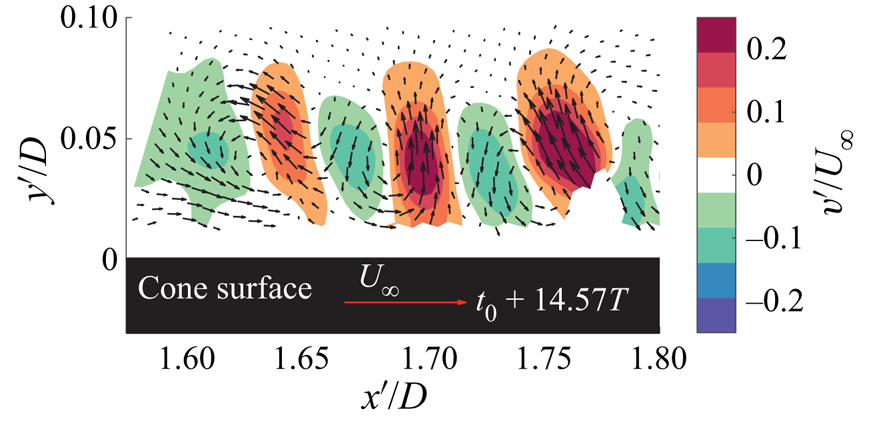
Figure 6. Instantaneous wall-normal velocity fluctuations with respect to the mean flow showing cross-sections of the spiral vortices (here  $\alpha =0^\circ$, operating condition I:
  $S_b=5$ and
  $Re_L=1.5 \times 10^4$); also see supplementary movie 1.
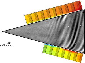
The growth of spiral vortices can be seen by tracking their evolution in time. Supplementary movie 2 shows the spiral vortices evolving over the rotating cone surface. A snapshot from this movie can also be seen in figure 7. The flow is from left to right, and the angular velocity is aligned with positive  $x$. The raw PIV recordings are processed such that the brighter regions signify higher seeding density. The seeding particles, being slightly heavier than air, get ejected outwards from the vortex cores due to the centrifugal force. Therefore, these vortex cores have low seeding density and appear as darker regions (marked as red dots). When tracking the spiral vortices as they move downstream, it appears that they have grown significantly after the maximum amplification point
  $l_m$ (corresponding to peak
  $I'_{rms}$).
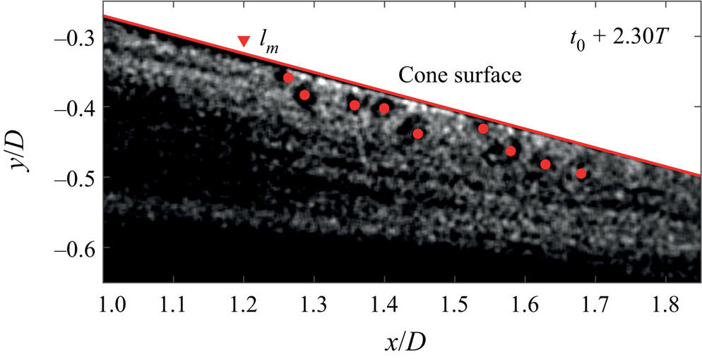
Figure 7. Spiral vortices as observed in a PIV recording. Image processing is applied to emphasise seeding density variations. The vortex cores are marked as red dots. Also see supplementary movie 2. (Here  $\alpha =0^\circ$, operating condition I:
  $S_b=5$ and
  $Re_L=1.5 \times 10^4$).
Figure 8 shows the spiral vortex evolution using three consecutive instants obtained from IRT measurements. Images on the right are the instantaneous temperature footprints of the spiral vortices. On the left, the traced values of  $I'$ along the
  $y/D=0$ are shown in combination with
  $I'_{rms}$. In the top row of figure 8, a batch of relatively strong vortices has just entered the amplification region at an instant of time
  $t_a=t_0+22T$. At
  $t_a+0.42T$, the footprint of the vortices has grown in amplitude. At the next instant
  $t_a+0.83T$, the amplitude has further increased. In this region a peak in
  $I'_{rms}$ is observed. Moving further downstream from the
  $I'_{rms}$ peak, the overall coherence decreases, i.e. the spacing between the vortices starts to vary around the circumference at a constant radius. Here, instances of vortex pairing are also observed.
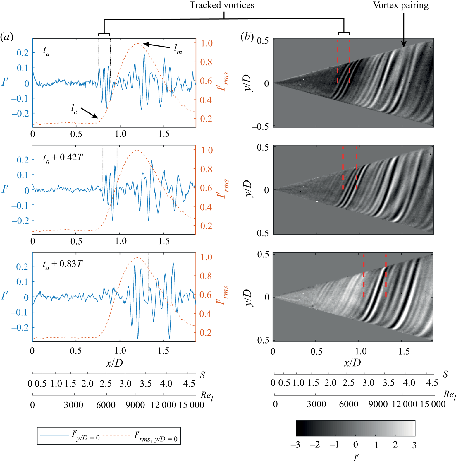
Figure 8. Instantaneous surface temperature footprints of the spiral vortices (b) and corresponding trace of intensity fluctuations  $I'$ at
  $y/D=0$ compared with
  $I'_{rms}$ over the dataset (a) (here
  $\alpha =0^\circ$, operating condition I:
  $S_b=5$ and
  $Re_L=1.5 \times 10^4$).
It is clear from figures 5 and 8 that the  $I'_{rms}$ peak represents the maximum amplification of the spiral vortices. Therefore, the point
  $l_m$ can be associated with the maximum amplification. The corresponding Reynolds number is defined as
 \begin{equation} Re_{l,m}=\frac{l_mu_e}{\nu}. \end{equation}
 The point  $l_c$ at which
  $I'_{rms}$ starts to grow is a critical point that represents the start of spiral vortex growth. The corresponding critical Reynolds number is defined as
 \begin{equation} Re_{l,c}=\frac{l_cu_e}{\nu}. \end{equation}
 In the present study, a closer inspection of figure 8 (right columns) shows that the spiral vortices appear at around  $x/D=0.5 \textrm {--}0.6$, which is before the critical point
  $l_c$ (around
  $x/D=0.78$) corresponding to the experimental value of the critical Reynolds number
  $Re_{l,c}=5.7 \times 10^3$ for the operating condition I. The accurate detection of the location where the spiral vortices originate is hindered by measurement limitations, because the spiral vortices are expected to be weak near their origin and their effect on the surface temperature may be below the measurement noise (
 ${<}25$ mK). Therefore, in the present study, the critical Reynolds number
  $Re_{l,c}$ is the Reynolds number that corresponds to a critical point at which the spiral vortices start to undergo a rapid growth, rather than a point at which they originate.
Since spiral vortex growth depends on local Reynolds number  $Re_l$ and rotational speed ratio
  $S$, the critical and maximum amplification locations for all the axial inflow cases are represented in the parameter space spanned by
  $Re_l$ and
  $S$; see figure 9. The grey lines (numbered as I to V) in figure 9 represent the variation of local Reynolds number
  $Re_l$ versus rotational speed ratio
  $S$ on the cone surface for different operating conditions. These lines can be used to relate the flow parameters (
 $Re_l$ and
  $S$) to the corresponding physical location on the cone surface.
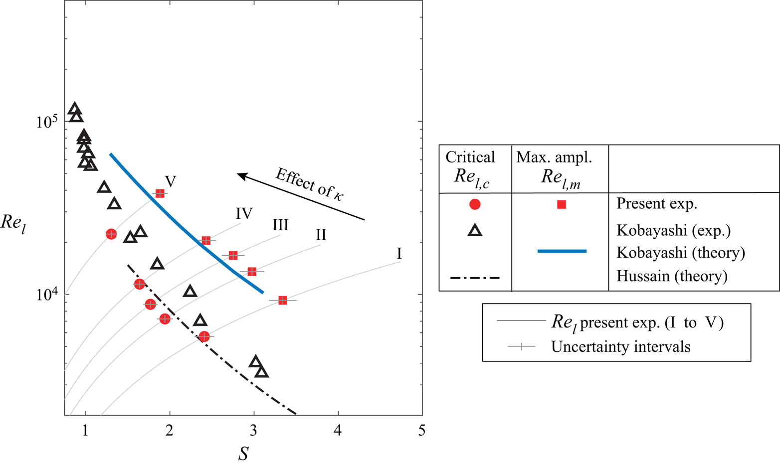
Figure 9. Comparison of  $Re_{l,c}$ and
  $Re_{l,m}$ measured in the present experiments with the data from the literature (Kobayashi et al. Reference Kobayashi, Kohama and Kurosawa1983; Hussain et al. Reference Hussain, Garrett, Stephen and Griffiths2016) for the cases with axial inflow: (I)
  $S_b=5$,
  $Re_L=1.5 \times 10^4$; (II)
  $S_b=4$,
  $Re_L=1.9 \times 10^4$; (III)
  $S_b=3.5$,
  $Re_L=2.1 \times 10^4$; (IV)
  $S_b=3$,
  $Re_L=2.5 \times 10^4$; and (V)
  $S_b=2$,
  $Re_L=3.7 \times 10^4$.
Figure 9 shows that the measured values of maximum amplification Reynolds number  $Re_{l,m}$ agree closely with the theoretical predictions of Kobayashi et al. (Reference Kobayashi, Kohama and Kurosawa1983). The values of the critical Reynolds number
  $Re_{l,c}$ fall closer to the measurements of Kobayashi et al. (Reference Kobayashi, Kohama and Kurosawa1983), and also agree well with the theoretical predictions of Hussain et al. (Reference Hussain, Garrett, Stephen and Griffiths2016). However, these values of
  $Re_{l,c}$ are nearly an order of magnitude higher than the theoretical predictions of Kobayashi et al. (Reference Kobayashi, Kohama and Kurosawa1983), which were based on the linear stability analysis (not shown here). Hussain et al. (Reference Hussain, Garrett, Stephen and Griffiths2016) argue that the theoretical predictions of the critical Reynolds number
  $Re_{l,c}$ are sensitive to the accuracy of computing the base flow over which the instability develops. With more accurate computations of the base flow, their theoretical predictions of
  $Re_{l,c}$ seem to closely agree with the experimental measurements. Similarly, Segalini & Camarri (Reference Segalini and Camarri2019) also highlight that the accurate computation of the base flow may play an important role in accurately predicting the stability characteristics over a rotating slender cone.
4.2. Non-axial inflow
Introducing a non-zero incidence angle significantly disturbs the symmetry of the flow field. Owing to the incidence angle, the edge velocity of the boundary layer (with respect to the cone surface) at a given axial location varies circumferentially, unlike in axial inflow. Figure 10(a) shows the meridional variation of the edge velocity measured by PIV for the cases of rotating and non-rotating cones at  $\alpha =0^\circ$ and
  $\alpha =4^\circ$. The comparison shows that, due to the incidence angle, the edge velocity is increased on the leeward meridian and decreased on the windward meridian. Consequently, the flow parameters, Reynolds number
  $Re_l^*$ and rotational speed ratio
  $S^*$, vary circumferentially at a fixed axial location, unlike in the axial inflow case. Here,
  $^*$ is used to denote the parameters obtained using the local edge velocities in the case of non-axial inflow. Additionally, there is a component of free-stream velocity in the
  $y$ direction. This, coupled with the cone rotation, adds to an asymmetry with respect to the
  $xy$ plane, dividing the regions into co-rotating and counter-rotating, as shown in figure 1. The conceptual difference in the tangential velocity profiles of the boundary layer at the counter- and co-rotating meridians is shown in figure 10(b) for the region where the tangential velocity of the cone surface is greater than the component of the outer flow velocity in the
  $y$ direction (shown for
  $|v_{\theta }|>|v_e|$). As a result, one can observe that the boundary layer profile is skewed to a larger extent on the counter-rotating meridian than on the co-rotating meridian. Consequently, the relative effect of rotation on the flow is higher in the counter-rotating meridian, analogous to coaxial cylinders rotating in opposite directions. Whereas, in the co-rotating meridian, the flow experiences a lower relative effect of rotation, analogous to coaxial cylinders rotating in the same direction. This effect can be accounted for by the variation in local rotational speed ratio as
  $S^*\approx (v_\theta -v_e)/u_e$, in the region where
  $|v_{\theta }|>|v_e|$.
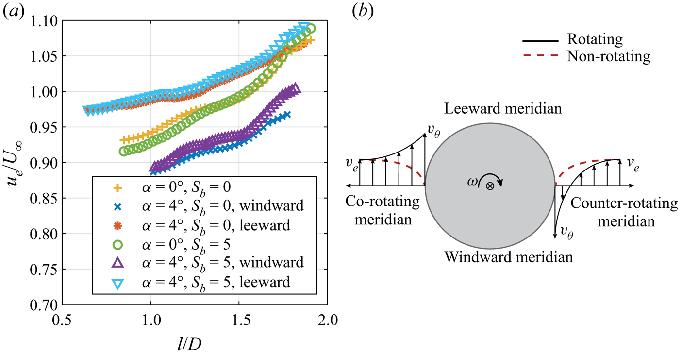
Figure 10. Asymmetry in the outer flow field. (a) Meridional variation of the boundary layer edge velocity. (b) Conceptual sketch of asymmetry in the boundary layer profiles between co-rotating and counter-rotating meridian, drawn at a cross-flow section of the cone (viewed from the cone apex).
It is clear that, due to the asymmetries in the velocity magnitude (leeward and windward meridians) and the relative velocity direction (counter- and co-rotating meridians), the local skewness of the boundary layer profile is distributed asymmetrically around the circumference. Therefore, at a fixed radius, this results in an asymmetric variation of local flow parameters ( $Re_l^*$,
  $S^*$) above and below the values corresponding to the axial inflow case at the same operating conditions, i.e. same inflow Reynolds number
  $Re_L$ and base rotation ratio
  $S_b$. Figure 11 shows these variations in local flow parameters (
 $Re_l^*$,
  $S^*$) at windward and leeward meridians in relation to the values from the axial inflow (
 $Re_l$,
  $S$) at the same operating conditions (
 $Re_L$,
  $S_b$). This shows that, along the cone meridians,
  $S^*$ and
  $Re_l^*$ follow the general trends of
  $S$ and
  $Re_l$, respectively, with small azimuthal variation. Additionally, the edge velocities required to estimate
  $Re_l^*$ and
  $S^*$ for all other investigated cases can be obtained using the fit parameters
  $C$ and
  $m$ from table 4 such that
  $u_e=CU_{\infty }l^m$.
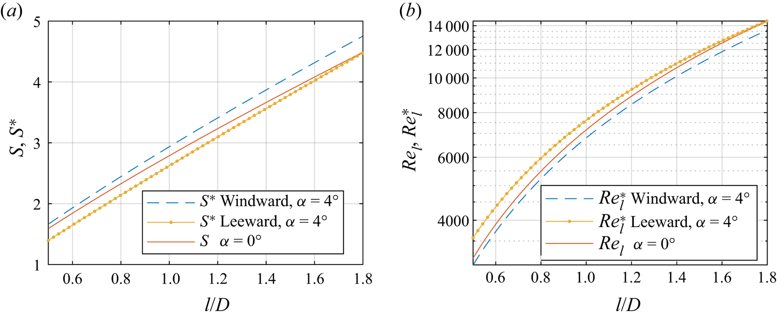
Figure 11. Correlation between the flow parameters from axial inflow ( $S$,
$S$,  $Re_l$ at
  $\alpha =0^\circ$) and non-axial inflow (
 $S^*$,
  $Re_l^*$ at
  $\alpha =4^\circ$) along cone meridians (operating condition I:
  $S_b=5$ and
  $Re_L=1.5 \times 10^4$).
Table 4. Fit parameters of the edge velocity  $u_e=CU_{\infty }l^m$ over the rotating cone.
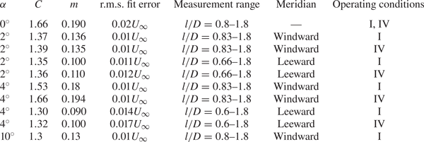
Generally, at constant  $Re_L$ and
  $\omega$, we can write
  $S^*(\theta ,\alpha ,l)=S(l) + \epsilon ^*_1(\theta ,\alpha ,l)$ and
  $Re_l^*(\theta ,\alpha ,l)=Re_l(l) +\epsilon ^*_2(\theta ,\alpha ,l)$. Here,
  $\epsilon ^*_1$ and
  $\epsilon ^*_2$ are deviations from the flow parameters for the corresponding axial inflow (
 $\epsilon ^*_1=\epsilon ^*_2=0$ when
  $\alpha =0^\circ$). It is clear that, due to the incidence angle, the distribution of the flow parameters (
 $Re_l$,
  $S$) around the cone gets distorted. The conceptual sketch of this distortion is shown in figure 12. It can be observed that the isolines of
  $S$ and
  $Re_l$ at a given location
  $l_1$ are coincident under axial inflow. At a non-zero incidence angle, these isolines become skewed. Consideration of this distorted distribution of the flow parameters is important for the discussion presented in § 4.3.
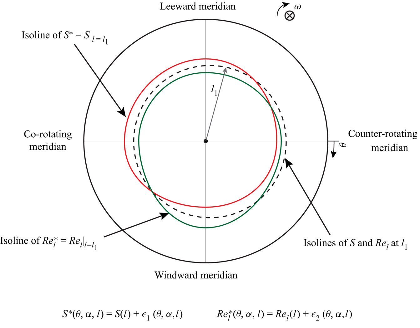
Figure 12. A conceptual sketch depicting the distorted distribution of the flow parameters  $S$ and
  $Re_l$ due to a non-zero incidence angle, shown as isolines of
  $S^*=S|_{l=l_{1}}$ and
  $Re_l^*=Re_l|_{l=l_{1}}$ at a given location
  $l_1$.
The asymmetry in the flow field has been found to have a significant effect on the formation and growth of the spiral vortices. Figure 13(c) shows the instantaneous surface temperature map over a rotating cone with the incidence angle  $\alpha =4^\circ$. It is important to observe that the spiral vortices are still present in asymmetric inflow conditions. However, their formation and growth are delayed to a location further downstream compared to the corresponding axial inflow case (compare points
  $l_c$ and
  $l_m$ in figures 13c and 5a).

Figure 13. Instantaneous surface temperature footprints of the spiral vortices over a rotating cone (c), and time-averaged velocity fields in the  $x'y'$ plane for rotating (b,d) case (
 $\alpha =4^\circ$, operating condition I:
  $S_b=5$ and
  $Re_L=1.5 \times 10^4$) as well as non-rotating (a,e) case (
 $\alpha =4^\circ$, operating condition VI:
  $S_b=0$ and
  $Re_L=1.5 \times 10^4$).
Figure 13 shows the corresponding time-averaged velocity field for both rotating (b,d) and non-rotating (a,e) cones under the same operating condition ( $\alpha =4^\circ$,
  $Re_L$ and
  $S_b$). When the cone is not rotating, the velocity field is asymmetric, with overall lower
  $x'$ velocity in the windward meridian. However, both windward and leeward meridians show a region of low
  $x'$ momentum close to the wall. When the cone is rotating, the mixing of high- and low-momentum fluid is observed close to the walls in both windward and leeward meridians, similar to the axial inflow conditions. As a consequence of the delayed growth of the spiral vortices, the mixing is also delayed to the downstream location with respect to the axial inflow case. Additionally, the mixing is more gradual in the leeward meridian than in the windward meridian. In the windward meridian, the
  $x'$ momentum is initially lower due to the incidence angle, but increases after the amplification of the spiral vortices.
Figure 13(c) also shows the loci of critical and maximum amplification points of the spiral vortex growth. These points are distributed at different radii around the cone due to the flow asymmetry, unlike in axial inflow. On the counter-rotating meridian, the critical and maximum amplification points are at lower axial locations ( $x/D=1.18$ and
  $x/D=1.41$, respectively); here, the deviation from the symmetric condition is expected to be highest (see figure 10b). The amplification on the leeward meridian occurs at the location with increased
  $x'$ momentum near the wall. However, on the windward meridian, the location where the
  $x'$ momentum starts to increase near the wall (around
  $x'/D=1.35$) appears to coincide with the critical point of the spiral vortex growth. In this region, the wall-normal velocity component is stronger and may play a role in delaying the local amplification of the spiral vortices; however, a separate investigation is required to further address this aspect. When comparing the location of amplification for the non-axial inflow to the axial inflow case, the location on the counter-rotating meridian is used.
Figure 14 shows the cross-sections of the spiral vortices in the windward and leeward meridians. Contours of wall-normal velocity fluctuations and vectors show the consecutive mutual upwash and downwash regions, similar to the axial inflow case (compare with figure 6). This confirms the counter-rotating nature of the vortices under non-axial inflow and, therefore, confirms the presence of the centrifugal instability.
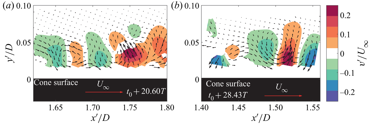
Figure 14. Instantaneous velocity fluctuations with respect to the mean flow showing cross-sections of the spiral vortices in (a) windward and (b) leeward meridians ( $\alpha =4^\circ$, operating condition I:
  $S_b=5$ and
  $Re_L=1.5 \times 10^4$). Contours represent the wall-normal velocity component. Also see supplementary movies 4 and 5.
Supplementary movie 3 shows spiral vortices evolving in the windward meridian; a snapshot from this movie can be seen in figure 15. The flow is from left to right, and the angular velocity of the cone is aligned with the positive  $x$ axis. The processed PIV images show the vortex cores as dark spots with lower seeding densities (marked as red dots), similar to that shown in supplementary movie 2. The vortex cores appear to grow significantly around the point
  $l_m$ (corresponding to peak
  $I'_{rms}$). Comparing supplementary movies 2 and 3 (or figures 7 and 15) shows that, in movie 3 (or figure 15), the spiral vortex growth has been delayed to a downstream location due to the non-axial inflow. Additionally, supplementary movies 4 and 5 show the time series of the vector fields shown in figures 14(a) and 14(b), respectively.

Figure 15. Spiral vortices as observed in a PIV recording. Image processing is applied to emphasise seeding density variations. The vortex cores are marked as red dots. Also see supplementary movie 3 (windward meridian,  $\alpha =4^\circ$, operating condition I:
  $S_b=5$ and
  $Re_L=1.5 \times 10^4$).
Additionally, a comparison of cases with different incidence angles ( $\alpha =0^\circ$ to
  $10^\circ$) is shown in figure 16. It is important to note that the spiral vortices appear and get amplified even in the non-axial inflow at the investigated inflow Reynolds numbers. The present observations are limited to the measured values of
  $Re_L < 2.5\times 10^4$.
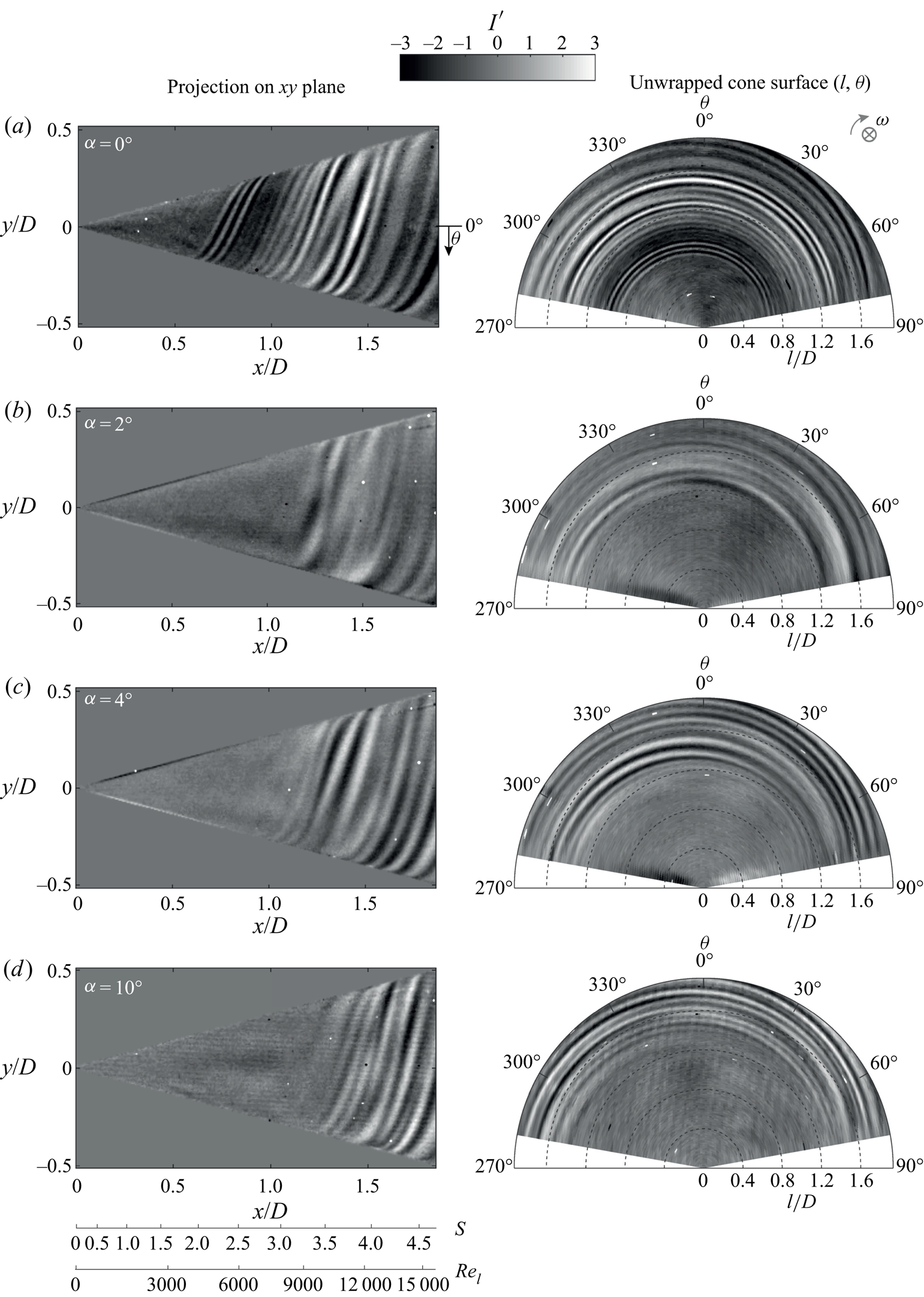
Figure 16. Effect of incidence angle variation on the instantaneous surface temperature footprints (at random instants) of the spiral vortices at operating condition I ( $S_b=5$ and
  $Re_L=1.5 \times 10^4$), counter-rotating meridian at
  $y/D=0$ for (a)
  $\alpha = 0^\circ$ (b)
  $\alpha = 2^\circ$, (c)
  $\alpha = 4^\circ$ and (d)
  $\alpha = 10^\circ$.
Figure 17 shows the effect of incidence angle on the (a) critical Reynolds number  $Re_{l,c}$ and (b) maximum amplification Reynolds number
  $Re_{l,m}$ measured on the counter-rotating meridian, and defined using the edge velocity of the corresponding axial inflow case at the same
  $Re_L$ and
  $S_b$. (Typical correlations between local flow parameters in axial inflow
  $S$ and
  $Re_l$, and non-axial inflow
  $S^*$ and
  $Re_l^*$, seen in figure 11, show that for large meridional shifts (changes in
  $l/D$) the flow parameters change by similar magnitudes in axial and non-axial inflow.) The important observation here is that even a small change in incidence angle greatly delays the critical Reynolds number, and, therefore, the amplification of spiral vortices. This is evident by observing that the extent of the delay is much larger when changing the incidence angle from
  $0^\circ$ to
  $2^\circ$ than from
  $2^\circ$ to
  $4^\circ$.
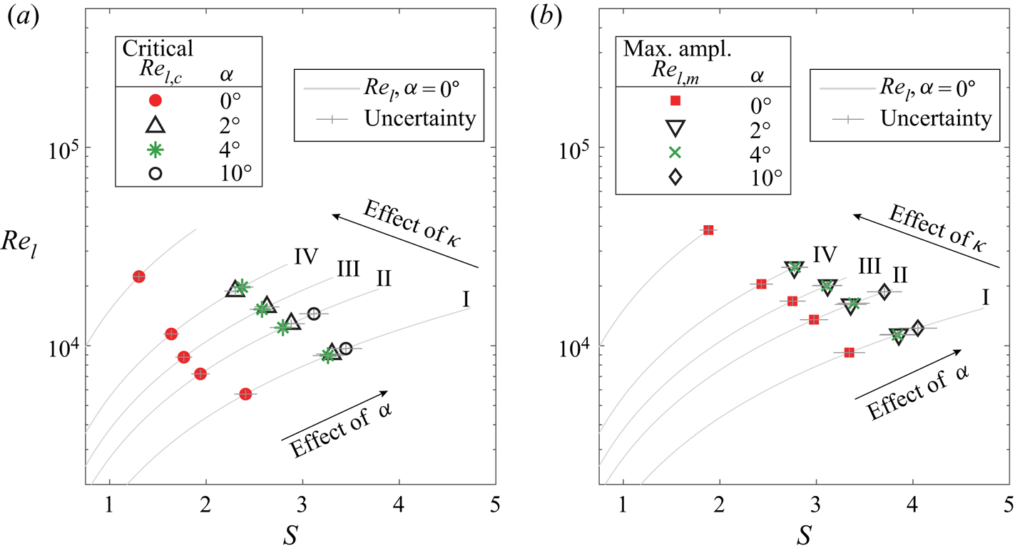
Figure 17. Effect of incidence angle on the (a) critical and (b) maximum amplification Reynolds numbers ( $Re_{l,c}$ and
  $Re_{l,m}$) shown on the scaling from the axial inflow cases (
 $Re_l$ and
  $S$) with the same operating conditions: (I)
  $S_b=5$,
  $Re_L=1.5 \times 10^4$; (II)
  $S_b=4$,
  $Re_L=1.9 \times 10^4$; (III)
  $S_b=3.5$,
  $Re_L=2.1 \times 10^4$; and (IV)
  $S_b=3$,
  $Re_L=2.5 \times 10^4$.
In figure 17, the critical and maximum amplification points corresponding to the case of  $\alpha =4^\circ$ appear at slightly lower rotational speed ratio
  $S$ as compared to the case of
  $\alpha =2^\circ$. This is a consequence of using the edge velocity field for the axial inflow case even for the non-axial inflow. Figure 18 shows the
  $Re_{l,m}^*$ and
  $S^*$ computed by using the edge velocity and locations of peak
  $I'_{rms}$ measured by observing windward and leeward meridian separately. Note that, at a meridian, the data points for
  $\alpha =2^\circ$ now appear at lower values of
  $S^*$ as compared to the case of
  $\alpha =4^\circ$. Along a meridian, the effect of increasing incidence angle on the vortices is monotonic, such that, with increasing incidence angle, the critical and maximum amplification locations appear at higher rotational speed ratios. Overall, the scaling in figure 17 can be used to highlight the significant differences between the symmetric and asymmetric flow fields.
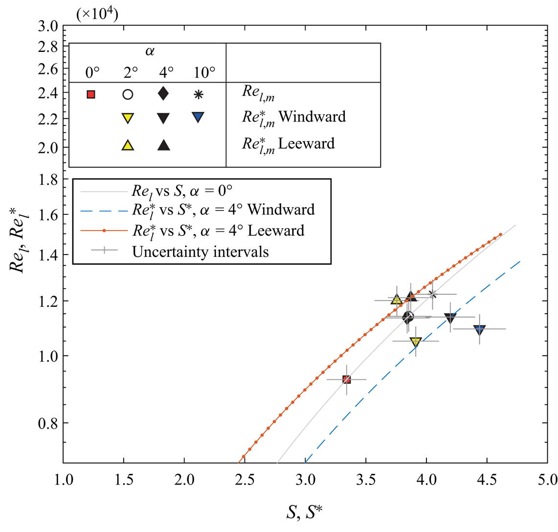
Figure 18. Effect of incidence angle on the maximum amplification Reynolds number, with the scaling obtained from the local edge velocity in the symmetry plane.
4.3. Physical interpretation
The delayed appearance and growth of spiral vortices in the non-axial inflow can be linked to the following aspects: azimuthal variations (at a constant radius) of the local flow parameters ( $Re_{l}^*$ and
  $S^*$), and, consequently, the variations in the azimuthal number (
 $n$) and angle (
 $\phi$) of the most amplified local perturbations that form the spiral vortices.
To obtain the vortex angle  $\phi$, extrema of
  $I'$ are tracked along the vortex (within
  $y/D=-0.07$ and
  $0.07$), for example, as shown in figure 19(a). The azimuthal number of vortices (counter-rotating vortex pairs)
  $n$ is obtained from the dark and bright fringes, as shown in figure 19(b). This procedure is repeated at various axial locations for all the cases investigated with IRT to cover a range of rotational speed ratio
  $S$. The invisible side of the cone in figure 19 is also investigated separately for all the cases of non-axial inflow.

Figure 19. An example showing how (a) spiral vortex angle  $\phi$ and (b) azimuthal number
  $n$ are extracted from the reconstructed surface temperature footprints (
 $\alpha =4^\circ$, operating condition I:
  $S_b=5$ and
  $Re_L=1.5 \times 10^4$).
Figures 20 and 21 show the variation of azimuthal number of vortices  $n$ and spiral vortex angle
  $\phi$ with rotational speed ratio
  $S$, respectively, for axial as well as non-axial inflow conditions. Since the rotational speed ratio
  $S^*$ circumferentially varies in non-axial inflow, and the complete three-dimensional velocity measurements around the rotating cone are unavailable here, the spiral vortex characteristics (
 $n$ and
  $\phi$) are presented against the rotational speed ratio
  $S$ from the corresponding axial inflow case (the typical correlation between
  $S$,
$S$,  $S^*$ and meridional location
  $l$ can be found in figure 11a). The overall trends of spiral vortex characteristics (
 $n$ and
  $\phi$) against the rotational speed ratio
  $S$ are similar for axial and non-axial inflows. Importantly, the values of
  $n$,
$n$,  $\phi$,
  $|\textrm {d}n/\textrm {d}S|$ and
  $|\textrm {d}\phi /\textrm {d}S|$ decrease with increasing rotational speed ratio
  $S$.
$S$.
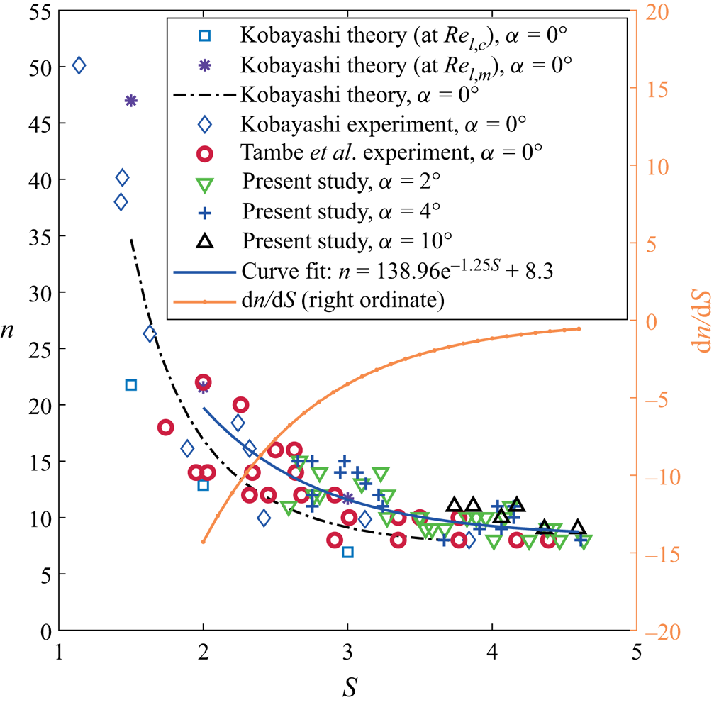
Figure 20. Azimuthal number of vortices  $n$ in non-axial inflow compared with the axial inflow cases from Kobayashi et al. (Reference Kobayashi, Kohama and Kurosawa1983) and Tambe et al. (Reference Tambe, Schrijer, Rao and Veldhuis2019).

Figure 21. Spiral vortex angle  $\phi$ for non-axial inflow compared with the axial inflow cases from Kobayashi et al. (Reference Kobayashi, Kohama and Kurosawa1983), Hussain et al. (Reference Hussain, Garrett, Stephen and Griffiths2016) and Tambe et al. (Reference Tambe, Schrijer, Rao and Veldhuis2019).
Generally, a range of perturbations with different wavelengths and orientations can grow in an unstable boundary layer, but the local flow conditions determine the wavelengths that can outgrow the rest (Drazin Reference Drazin2002). Over a rotating cone, an additional constraint restricts the azimuthal wavelengths ( $\lambda _{\theta }$) that may grow such that there is an integer number (
 $n$) of spiral vortices around the cone at a given radius; because any remaining fraction of a wave cannot sustain as a vortex. For an axial inflow, the local flow parameters (
 $S$ and
  $Re_l$) are constant along the azimuth for a given radius. Ideally, this condition allows the growth of the same wavelength (such that
  $\lambda _{\theta }/r=2{\rm \pi} /n$) at the same angle (
 $\phi$) around the azimuth (at a given radius). However, in non-axial inflow, the local flow parameters (
 $S^*$ and
  $Re_l^*$) azimuthally vary at a given radius. Moreover, their isolines are skewed (as shown in figure 12). Such locally varying conditions can give rise to different wavelengths at different orientations around the azimuth, which can inhibit the formation of azimuthally coherent spiral vortices.
The non-axial inflow significantly disturbs the azimuthal coherence of the instantaneous spiral vortex footprints. This is evident from figure 22, which shows the unwrapped surfaces of a rotating cone for axial and non-axial inflow. In the axial inflow case (figure 22a), the spiral vortex footprints show strong coherence (less azimuthal variation in spacing and orientation) from  $l/D=0.6$ to their maximum amplification at
  $l/D=1.24$, after which the coherence decreases. Figures 22(b) and 22(c) are uncorrelated instants from separate measurements on opposite sides of the cone at
  $\alpha =4^\circ$. Here, the local flow parameters
  $S^*$ and
  $Re_l^*$ vary azimuthally, as shown at the windward (
 $\theta =90^\circ$) and leeward (
 $\theta =270^\circ$) meridians for figures 22(b) and 22(c). Consequently, the vortex footprints show an overall weak azimuthal coherence, as their spacing and orientation vary along the azimuth. Additionally, the critical and maximum amplification loci also show significant azimuthal variations, in contrast with the axial inflow, where there is no such azimuthal variation.
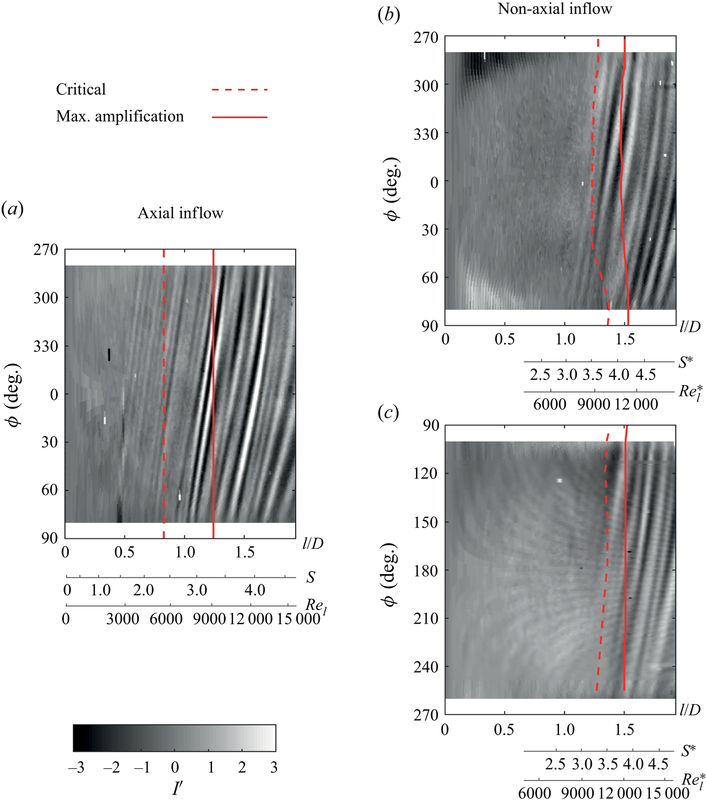
Figure 22. Comparison of the spiral vortex footprints over the unwrapped cone surface for  $\alpha =0^\circ$ (a) and
  $\alpha =4^\circ$ (b,c, as uncorrelated instances) at operating condition I:
  $S_b=5$ and
  $Re_L=1.5 \times 10^4$.
Relating to the cases from figure 22, the azimuthal variations in the local instability characteristics are shown in figure 23. The most amplified perturbation waves are schematically shown at leeward and windward meridians (figure 23b–d). The azimuthal differences (between leeward and windward meridians) of vortex number  ${\rm \Delta} n$ and angle
  ${\rm \Delta} \phi$ (figure 23a) are estimated using the experimental data (figures 20 and 21), where the respective trends of
  $n$ and
  $\phi$ versus the rotational speed ratio
  $S$ agree for axial and non-axial inflow (for
  $S=2.5\text {--}4.6$). For the purpose of estimation, the local values of
  $n$ and
  $\phi$ are obtained by replacing
  $S$ with
  $S^*$ in the curve fits (figures 20 and 21). This approximation is based on the assumption that the local effects of rotation (relative to the edge velocity) on the local instability characteristics are similar in axial and non-axial inflow, e.g. stronger rotation (higher
  $S$ or
  $S^*$) promotes longer azimuthal wavelengths (lower
  $n$), with their wavefronts oriented more towards the tangential velocity of rotation (lower
  $\phi$). These approximate estimates in figure 23(a) should only be interpreted for their qualitative trends. Here, both
  ${\rm \Delta} n$ and
  ${\rm \Delta} \phi$ are large initially (at
  $l/D<1.35$), which suggests a large variation in the most amplified perturbation waves around the azimuth, as depicted in figure 23(c). This is the region where no vortices are observed (
 $l/D<1.35$ in figures 22b and 22c). Further downstream (where overall
  $S^*$ values increase), the differences
  ${\rm \Delta} n$ and
  ${\rm \Delta} \phi$ decrease, suggesting that similar perturbation waves can grow around the azimuth (see figure 23d), similar to the axial inflow case (figure 23b). This is the region where the spiral vortices are observed. This shows that, at increased rotational speed ratios, azimuthal coherence is approached, which promotes the growth of the spiral vortices around the cone surface in the non-axisymmetric flow field.
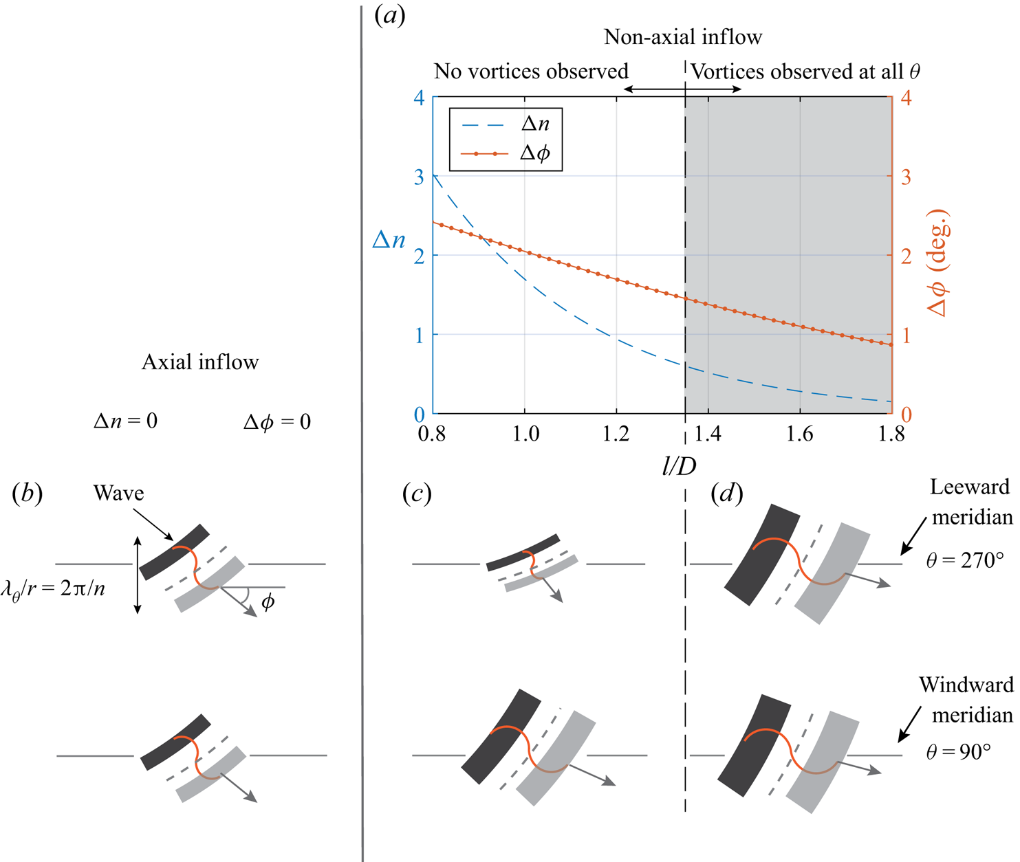
Figure 23. Azimuthal differences (between leeward and windward meridians) in vortex number  $n$ and angle
  $\phi$ shown as (a) estimates for
  $\alpha =4^\circ$, at operating condition I (
 $S_b=5$ and
  $Re_L=1.5 \times 10^4$), and as schematic waves for (b) axial and (c,d) non-axial inflow.
5. Conclusions and discussions
The spiral vortices, induced by the centrifugal instability, over the rotating slender cone ( $\psi =15^\circ$) were visualised by their surface temperature footprints, obtained by IRT coupled with the POD approach. Incidence angles
  $\alpha =0^\circ$,
  $2^\circ$,
  $4^\circ$ and
  $10^\circ$ were investigated. The measured surface temperature fluctuations show the growth of spiral vortices over a rotating slender cone. For axial inflow, the critical and maximum amplification locations of the spiral vortex growth (in parameter space of Reynolds number and rotational speed ratio) agreed with the past literature, validating the approach.
The conclusions are summarised as follows.
(i) The asymmetry of the non-axial inflow inhibits the initial growth of the spiral vortices. However, spiral vortices, induced by the centrifugal instability, were detected at a higher local rotational speed ratio
 $S$ and local Reynolds number $Re_l$ as compared to the corresponding axial inflow case.
(ii) The azimuthal variation of local Reynolds number and rotational speed ratio in non-axial inflow causes azimuthally varying instability characteristics (azimuthal number
$n$ and angle $\phi$ of the most amplified perturbations). It is postulated that these variations may inhibit the growth of azimuthally coherent spiral vortices.(iii) However, at a higher local rotational speed ratio, the instability characteristics (azimuthal vortex number
$n$ and vortex angle $\phi$) become less sensitive to the changes in local flow parameters, which allows the spiral vortices to grow.


It should be noted that the present study does not deny other possible phenomenological differences (different instability mechanisms) in asymmetric flow around the rotating cone. However, such phenomena, caused by asymmetry itself, are expected to be azimuthally incoherent. The centrifugal instability appears to be overall dominant in the region with increased azimuthal coherence of its instability characteristics. Understanding other secondary phenomena and their relative importance with respect to the observed centrifugal instability needs a separate investigation.
Although the investigations in this study are of fundamental nature, the results are relevant for various engineering applications in which a rotating slender cone faces non-axial inflow. In novel aircraft propulsion concepts, aero engine spinners may face a non-axial inflow when the embedded engines ingest the airframe boundary layer, or when the flow separates in the short intakes of ultra-high-bypass-ratio engines. In these cases, spiral vortices may still appear over a rotating slender cone, but their formation and growth will be delayed to a downstream location compared to the axial inflow at the same operating conditions. These vortices can alter the distortion and blade incidence angles at the blade–hub junction, thus changing the loss mechanisms. However, the inflow Reynolds number ( $Re_L \leqslant 2.5 \times 10^4$) and Mach number (
 $M<0.02$) of the present study do not cover the whole range of the flow conditions encountered in aviation. In this regards, investigating the Reynolds-number and Mach-number effects on the boundary layer instability over a rotating cone is still an open question. Moreover, the boundary layer instability over cones of different half-angles rotating in axial or non-axial inflow has still not been experimentally investigated. This is particularly challenging because, between half-angles
  $30^\circ$ and
  $40^\circ$, the instability mechanism changes from the centrifugal to the cross-flow (Kobayashi Reference Kobayashi1994).
Supplementary movies
Supplementary movies are available at https://doi.org/10.1017/jfm.2020.990.
Acknowledgements
We thank Professor Dr Ing. G. Eitelberg for intriguing discussions and encouragement. This work was funded by the European Union Horizon 2020 programme: Clean Sky 2-Large Passenger Aircraft (CS2-LPA-GAM-2018-2019-01), and CENTERLINE (grant agreement no. 723242). We also thank the reviewers for their valuable feedbacks which improved the quality of this paper.
Declaration of interests
The authors report no conflict of interest.


 Open access