Forecasting Model and Related Index of Pig Population in China

1
Department of Industrial Engineering, College of Engineering, Northeast Agricultural University, Harbin 150030, China
2
Department of Agriculture and Forestry Economics and Management, School of Economics and Management, Northeast Agricultural University, Harbin 150030, China
*
Authors to whom correspondence should be addressed.
†
These authors contributed equally to this work.
Symmetry 2021, 13(1), 114; https://doi.org/10.3390/sym13010114
Submission received: 1 December 2020
/
Revised: 5 January 2021
/
Accepted: 7 January 2021
/
Published: 11 January 2021
Abstract
:The systematic and reasonable prediction of pig population is the basis for balance and symmetry between the supply and demand of hogs, which is of great significance to the pig industry. Based on the population prediction model and according to the principle of pig months transfer, this paper referred to the modeling principle and method of the discrete population quantity prediction model and established a related index model that can reflect the pig population development process. The forecasting model we have established includes the following models: (a) a recursive model of pig population, (b) an estimation model of new kept piglets and breeding sows in each month, (c) an estimation model of the initial state of the quantity of the pig population, and (d) a related index model to calculate pig population. On this basis, an example calculation was made to predict the monthly pig population and the quantitative distribution of pigs with different age groups in China from January 2016 to March 2018 in the future. The results showed that the forecasting model of pork supply based on the prediction of pig population is an effective perspective to study the future quantity of pork supply. In the fitting stage, the relative error of the number of slaughtered fattened hogs was 0.0332 and 0.0368. In the prediction stage, the relative error of the quantity of pork supply was 0.0618 and 0.0578.
1. Introduction
With the deepening of market-oriented reforms and the accelerating process of internationalization, various traditional and non-traditional risks are constantly increasing, and the hog price is in a state of cyclical fluctuations. Fluctuation of hog price will not only damage the interests of producers but also harm the interests of consumers. At the same time, it can lead to an imbalance in the development of the national economy and an asymmetric input and output. In this case, a system that enables the proper control of pig population has become an urgent problem to be solved, because it can make the supply and demand of hog balance symmetrical and thus reduce the large fluctuations in hog price.
According to the existing literature review, there are few studies that include calculation of pig population. Most of the research slightly mentions models that calculate pig population from the perspective of hog price forecasts. Current research studies mainly include one-factor prediction and multi-factor prediction from the aspect of the factors considered. In terms of one-factor prediction, it uses the hog price itself or some other single factor such as the ratio of breeding sow stocks or hog–grain price as the explanatory variable [1,2,3]. The multiple-factor prediction use factors such as piglet prices, the body size parameters, and hog–grain ratio together or daily settlement futures, options prices, and feed prices (maize price and international soybean price) for lean hogs as explanatory variables to predict hog prices [4,5,6]. These methods are all general methods with a wide range of application and low specificity.
Current research into hog prices focuses on static prediction and dynamic prediction from the aspect of the research method. In terms of static prediction, according to the historical data of agricultural products such as hog prices, scholars screen out the influencing factors that affect the fluctuation of hog prices [7] and find out the fluctuation of hog prices through theoretical analysis [8,9,10]. Linear regression prediction has been applied to predict price fluctuations such as the regression analysis, the multiple linear regression method, and econometric modeling [11,12,13,14,15,16,17,18,19,20,21,22]. Then, the artificial intelligence (AI) tools have been applied to deal with the problem of agricultural commodity price forecasting [23,24,25,26,27,28,29,30].
Although the existing research has different perspectives, it is obvious that the major cause of fluctuation in hog price is the variation in supply. Reasonable prediction of the hog supply is fundamental to control fluctuations in pork prices. In recent years, Ref. [31] pointed out that the use of data on the pig population in the pig population management system can improve the prediction accuracy of pig supply. Therefore, the pig population prediction is the basis and premise for understanding and controlling the production capacity of pork. At present, there are few studies on the prediction of pig population. Ref. [32] developed a system dynamics model as a tool for managing and visualizing changes in pig population. The model can be used to simulate the expansion and contraction of the pig population with the influencing factors such as increasing the number of sows. This model can roughly visualize the changes of a pig population without the need for in-depth basic mathematics. There are some scholars concerned with the predictions about certain kinds of pigs such as making a preliminary prediction on the number of breeding sows based on historical data to point out that the number of breeding sows would continue to decline for about 3 months. Some authors also pointed out that there is a quantitative causal relationship between the number of sows and the price of pigs, but the specific quantitative relationship has not been calculated, and no corresponding functional model has been established [33,34].
The PPM (population prediction model) [35] is a useful evolutionary approach that can explore good solutions for complex problems such as the prediction of pig population. In fact, according to the population control theory, slaughtered pigs are grown from new born piglets, growing slaughter pigs to fattening pigs, while the new born piglets are bred by sows. Therefore, as long as the current number of breeding sows can be controlled, the amount of pig population at a certain time in the future can be determined or predicted. Therefore, using the PPM theory, it is possible to solve the problem of in a short prediction time and also control and predict the number of pigs of different ages at any month. However, unlike PPM, pig population predictions are more complicated. For example, the number of births of the people population can be adjusted according to the policy. Yet the pig population seems to be much more controllable than any human population.
Therefore, a prediction method that is a mechanism model for predicting the number distribution of pig population based on PPM is proposed. Specifically, a method to establish a correlation model between the price of pork and the number of new born gilts is also designed. According to the existing statistical data and the growth characteristics of pigs, the estimation methods of new kept gilts and capable sows in each year and how to determine the initial state of the pig population is presented.
2. Model Building
2.1. Pig Type and Growth Stage
In order to accurately study the distribution of the number of pigs in each category, the month is the minimum time unit for the growth process of the pigs. That is, the growth time of the pigs is calculated by the month age. Based on the definition of existing research and statistical yearbooks at this stage, this paper defines the growth stages of various types of pigs.
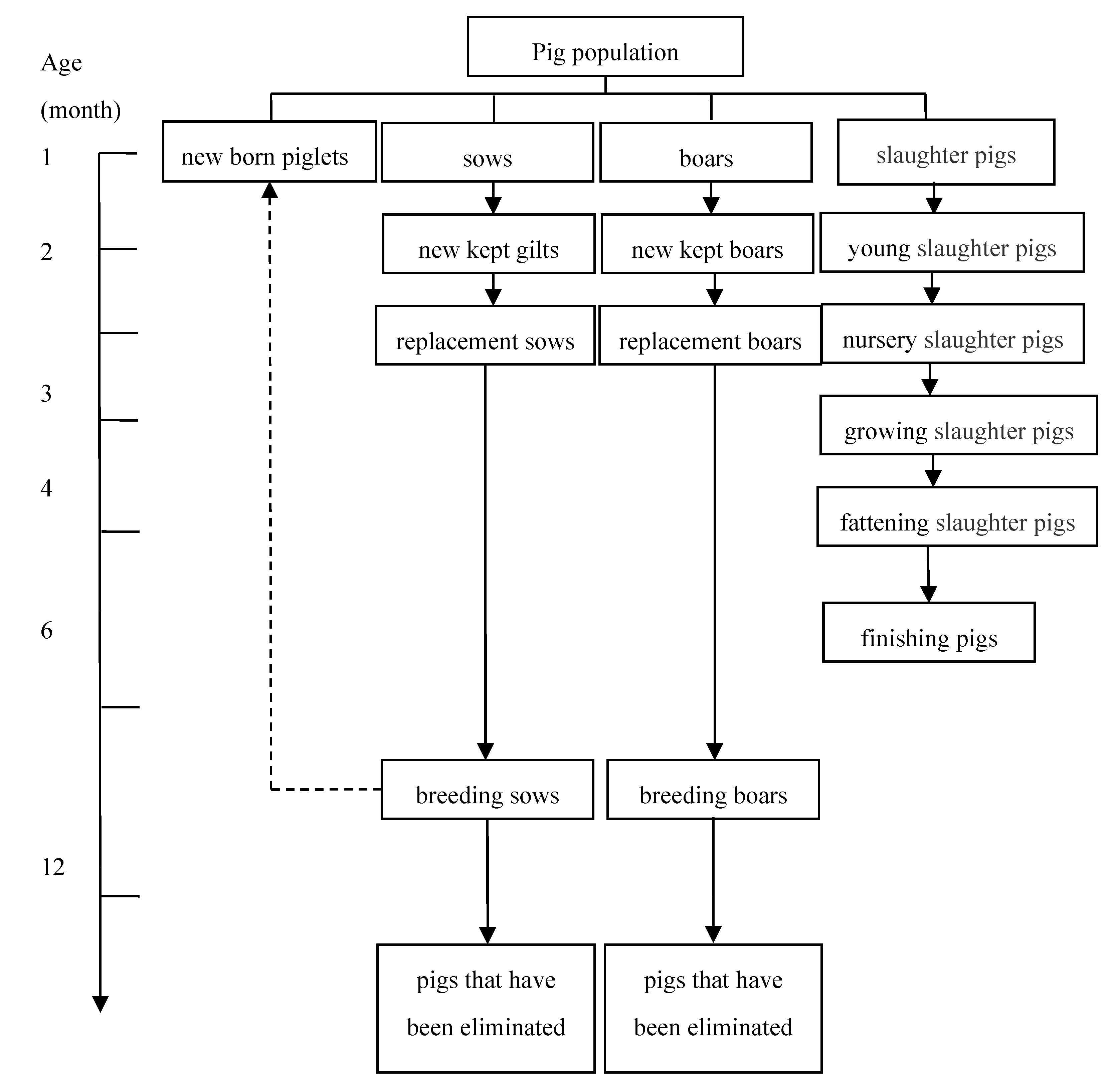
The pig population consists of four types of pigs, namely new born piglets, sows, boars, and slaughter pigs. Among them, new born piglets are bred by breeding sows; that is, new born piglets are less than one month old. When it grows to 1 month of age, it is divided into three categories according to production functions: sows, boars, and pigs. Among them, sows are female pigs of any age to give birth to the piglet, and their growth stages can be divided into: new gilts, reserve sows, and breeding sows. A boar is a male pig that is not castrated and that is specifically used to mate with multiple sows. Similar to the definition of sows, its growth stages can be divided into new kept boars, replacement boars, and breeding boars. The phrase ‘slaughter pigs’ refers to pigs that provide meat after being slaughtered. Its growth stages can be divided into young slaughter pigs, nursery slaughter pigs, growing slaughter pigs, fattening slaughter pigs, and finishing pigs. In summary, according to the age distribution of the population, a schematic diagram of the pig population is obtained (Figure 1).
It should be noted that this study takes the content of statistics of animal husbandry in the China Statistical Yearbook as the research standard and official data source. So, with reference to the Chinese census structure in the China Statistical Yearbook, this study considers that breeding sows are sows who have given birth to one gilt and can continue to reproduce normally. The Ministry of Agriculture and Rural Affairs-Technical specifications for ear tags for breeding sows stipulates that sows older than 8 months have reached the breeding age and can be mated. After the first gestation period of about 114 days, sows over 12 months old will become breeding sows. The breeding sow can be mated for 3.5 years, so the maximum age of breeding sows is 54 months.
2.2. Derivation and Establishment of the Recursive Model of Pig population and Estimation Model of Pork Supply
If the number of pigs in a certain month is counted by month, that is, the total number of sows that are months old but less than months old at time is , r takes the integer 1,2,3… etc. Among them, the breeding sows interval of the fertile sows is , the minimum age of that can be used for sows is generally 12, and the maximum age of is generally 54. When is the number of piglets produced by the sows, the average number of pigs per year can be produced in one month at the time and months old, and F is the total number of piglets that can be produced by the sows at the time of and months old.
If changes from to , sum , and the total number of piglets that can be bred by all the sows at time is .
When
where is the pattern of pig population growth, indicates the total number of litters per breeding sow in the entire breeding interval at month , and A is the number of piglets per litter, we obtain the result
Then, the number of piglets less than one month old in the new born piglets and the number of piglets between 1 and 2 months old at time are as follows:
In Formulas (7) and (8), is the mortality rate of new born piglets, and is the mortality rate of new born piglets less than 1 month old.
When the new born piglets grow to the age between 1 and 2 months old, the pig farmer will classify them into three types: boars, sows, and slaughter pigs according to their production functions. Let the total number of pigs growing from new born piglets to 1 month old at time be and the number of new gilts selected from 1 month old piglets at time be . Then, at time , the number of new kept boars at the age of 1 month and the number of small slaughter pigs at the age of 1 month are as follows:
In Formula (9), is the ratio of the number of sows to boars selected for piglets of one month old.
According to Formulas (8)–(10), at the age of 1 month, the number of sows, boars, and hogs at r + 1 month of age are as follows:
In Formulas (11)–(13), is the number of r months of age sows at time , is the number of months of age boars at time , is the number of months of age slaughter pigs at time , is the mortality rate of months of age sows, is the mortality rate of months of age boars, is the mortality rate of months of age slaughter pigs, is the maximum months of age for mating with boars, and is the average months of age of pork pigs.
The above model is a recursive model that can be recursed to any subsequent month. In fact, the pig population is a process of constant transfer, and the number of pig population in a month is the number of pigs in the last month after death and elimination. In addition, in the basic idea of PPM, predictions can also be divided into purely natural predictions and predictions with disturbances. The so-called disturbances here mainly refer to mechanical changes, such as the possible natural disasters such as African swine fever, which disturb the development process of the pig population. This disturbance has great contingency and randomness. Therefore, a random disturbance term is set to represent such mechanical changes.
In summary, the formulas for recursive by category and number of months of age pigs are as follows:
- The recurrence formula of the distribution of the number of new born piglets by months of age is as follows:
- The recurrence formula for the distribution of sows by months of age is as follows: is the number of artificially retained.
When a sow grows to 12 months of age, it becomes a breeding sow. The number of breeding sows is .
- 3.
- The recurrence formula for the distribution of boars by months of age is as follows:
- 4.
- The recurrence formula for the distribution of the number of pork pigs per month of age is as follows:
When a slaughter pig grows to 6 months of age, it becomes a finishing pig, that is, .
2.3. Estimation Method for New Kept Gilts and Breeding Sows
2.3.1. Estimation of the Sum of Monthly Mortality and Culling Rate of Breeding Sows
There are not only natural mortality rates but also artificial elimination rates for breeding sows. Let indicate the sum of the maternal mortality and culling rate per year, indicate the mortality rate of the annual breeding sows, indicate the elimination rate of the annual breeding sows, indicate the sum of mortality and elimination rate of r months of age breeding sows, indicate the mortality rate of breeding sows, and indicate the elimination rate of r months of age breeding sows. Then, and are as follows:
In the current study, there are only statistical data on the sum of annual mortality and elimination rate of breeding sows, but there are no statistical data on the sum of monthly mortality and elimination rate for breeding sows. The sum of monthly mortality and elimination rate of breeding sows is the basis of the subsequent estimation method for new kept gilts. Therefore, this paper tries to establish the relationship between the sum of mortality and elimination rate of breeding sows per year () and the sum of mortality and elimination rate of monthly breeding sows (). Then, the sum of mortality and elimination rate of breeding sows can be determined each month.
Based on the calculation method of population mortality in the China Statistical Yearbook, the estimated value of annual mortality and elimination rate of breeding sows is the ratio of the number of breeding sows dead and eliminated in one year to the number of breeding sows dead and eliminated in the middle of the same period, which is expressed by the percentage of 1000, as shown in Formula (20). It should be noted in particular that the breeding sows are eliminated immediately when they reach the age of 54 months, that is, the total number of breeding sows that the breeding sows whose age is 54 months is not included in the total number of breeding sows in t month. Meanwhile, the number of breeding sows eliminated and dead in t month included the number of breeding sows eliminated at 53 months of age in t−1 month and the number of breeding sows that were eliminated after the t month grew to 54 months of age, as shown in the following formula:
In Formula (20), represents the number of breeding sows in the month of January at months of age in years. The first item indicates the number of eliminated breeding sows at 12 months of age per month from January to December in year, the fourth item indicates the total number of breeding sows that have reached the age of 54 months. Among them, the number of breeding sows at 12 months is as follows:
In Formula (21), is the sum of the mortality and elimination rate of the non-breeding sows at r months. In summary, taking the minimum error between the actual value and the estimated value of annual mortality and elimination rate as the goal, that is , we constructed a model for calculating the sum of mortality and elimination rate of monthly breeding sows. According to expert consultation, the sum of the annual mortality rate and the elimination rate of the breeding sows can be 40%. Assuming that the newly kept gilts in each month are a fixed value , and under the condition of , = 0.01735 can be obtained.
2.3.2. Calculation Method for New Gilts in Each Month
Construction of the Relationship Model between New Kept Gilts and Pork Prices
According to the Encyclopedia of Agribusiness [36], “pig cycle” is understood as the following: a decrease in profitability causes farmers to lose interest in breeding pigs. As a consequence, the stocks of sows are reduced. In time, it results in decreased stocks of piglets. According to the theory of “pig cycle”, pork production often depends on the producer’s response to price in production practice. Therefore, when the price of pork rises, the producers will increase their enthusiasm for breeding pigs and keep more sows for breeding piglets. Then, the number of pigs that they breed will increase, and the economic returns of the output of pork will increase, too. However, when the price of pork rises falls, the producer’s enthusiasm for breeding is weakened. Then, the producer will keep fewer gilts. So, the numbers of piglets will be reduced, too.
Since there is still a lack of research on the influencing factors and estimation model of new kept gilts, this paper is an initial exploration of the factors affecting the number of new kept gilts. This paper attempts to select the most direct factor affecting the new kept gilts—pork prices—and establishes a relationship model between pork prices and new kept gilts. In summary, this paper proposes the following assumptions:
Formula (22) refers to the number of new kept gilts in the first month of the year (that is, the 1-month-old gilts that are kept in the new born piglets in each month of the year), which is the pork price in the first year of the month. In Formula (22), all variables are unknown except pork prices. Therefore, how to calculate parameters a and b in Formula (22) is a problem that needs to be solved.
Parameter Calculation of the Relationship Model between New Kept Gilts and Pork Prices
The values of parameters a and b in Formula (22) cannot be calculated by linear regression, but they can be calculated by establishing a relationship model between the breeding sow and the new kept gilts. The breeding sows are grown by the new kept gilts, and there is a quantitative relationship between them. Then, the relationship formula between the new kept gilts and the price of pork can be brought into this relationship model. All the data needed by the model, including the annual numbers of breeding sows and pork price, can be accessible. In this way, parameters a and b in the model of the relationship between the new gilts and pork prices can be calculated.
The current statistics on the number of stocks of breeding sows per year are counted from the end of the year. Therefore, this paper establishes the relationship between the number of breeding sows at the end of the T + 1 year. The formula mainly includes three items. The first item is the number of breeding sows that can experience death and elimination in the T year and grow to the end of the T + 1 year. The second item is that the new kept gilts in T + 1 in January will experience 11 months. According to their monthly mortality and elimination rate, they will grow to 12 months of age at the end of T + 1 and join the breeding sows. The third item is that the new kept gilts from February to December in T year will become breeding sows in the next year, according to their monthly mortality and elimination rates. According to the above relationship, the number of breeding sows at the end of the T + 1 year can be estimated as follows:
Substitute Formula (22) into Formula (23), and finishing:
When:
Then, the formula can be written as follows:
If the estimated value of is recorded as , . Let . According to the principle of least squares, the result can be obtained as follows:
2.3.3. Estimation of Breeding Sows at Each Month of Age
In summary, the estimated models for the breeding sows at each month of age are as follows:
2.4. Estimate of the Initial Condition of the Pig Population
The initial state of the population is the basic data for the prediction of pork supply and is also a prerequisite for prediction. In order to predict the pork supply, it is necessary to obtain the basic data of the initial state of the population, but there are no annual statistics for these data. Therefore, the initial state of the population needs to be estimated. The initial status of the pig population includes new born piglets, sow populations, boar populations, and slaughter pig population. All kinds of pigs are recursed monthly according to their monthly mortality. Each month, new piglets that can breed sows are added to the pigs. The above estimates the number of breeding sows per month by establishing a monthly estimation model. Therefore, if the base month is t, the initial state of the new born piglet in month t is as follows:
The above estimates the number of new gilts in each month by establishing a monthly estimation model. According to the transfer principle of the pigs by the age of the month, the distribution of the number of sows per month can be estimated. Then, the initial state of the sow population in months is as follows:
The proportion of producers who keep boars and sows is k. Therefore, the initial state of the boar populations is as follows:
The breeding pigs can breed new piglets. After the new born piglets grow to 1 month of age, the farmers decide the number of new gilts who are left according to the current pork price and choose the new kept boars for breeding, and the rest are used as slaughter pigs who will be slaughtered after 6 months of age. Therefore, the initial state of the slaughter pig population is as follows:
2.5. Population Index
In some cases, in order to describe certain characteristics of the population development process and use them for the statistics of the population, it is necessary to introduce some mathematical features (called the population index), which are directly related to . The formula for calculating various population indices is as follows:
Pigs under the age of 2 months are collectively referred to as new born piglets. When the new born piglets grow to 1 month of age, they are classified into sows, boars, and pigs according to different production functions. Each type of pig has its own growth stage. The growth stages of sows are nursery sows, growing sows, and breeding sows. The growth stages of boars are nursery boars, growing boars, and breeding boars. The growth stages of the slaughter pigs are divided into nursery slaughter pigs, growing slaughter pigs, fattening slaughter pigs, and slaughter pigs. In addition to studying the various stages of different types of pigs, this paper presents the distribution of the number of pigs in each category by month.
- (1)
- Number of breeding sows at the end of the year:
- (2)
- Inventory of pigs at the end of the year:
- (3)
- Number of slaughtered fattened hogs
- (4)
- Pork production in the current year:
- (5)
- Number of sows per month at time t:
Number of new kept gilts:
Number of replacement sows:
In this formula, is the maximum age of the replacement sows, which is the minimum age of breeding sows, and is the minimum age of the replacement sows.
The number of breeding sows is as follows:
In this formula, is the maximum age of breeding sows.
The total number of sows is as follows:
- (6)
- Number of boars per month age at time t
The number of new kept boars is as follows:
The number of replacement boars is as follows:
is the age of the new born piglets when it is raised as a replacement boar. is the maximum age of the replacement boar, and is the minimum age of the breeding sow, too.
The number of breeding boars is as follows:
In this formula, is the maximum months of age of breeding boars.
The total number of boars is as follows:
- (7)
- The number of boars at time t
The number of small slaughter pigs is as follows:
The number of nursery slaughter pigs is as follows:
In this formula, is the month of age of the piglet when it grows to nursery slaughter pigs, and is the maximum month of age of nursery slaughter pigs.
The number of growing slaughter pigs is as follows:
In this formula, is the maximum month of age of growing slaughter pigs.
The number of fattening slaughter pigs is as follows:
In this formula, is the age of the fattening pork pig when it is raised as a finishing pig.
The number of finishing pigs is as follows:
The total number of pork pigs is as follows:
If the average amount of meat produced after slaughtering a pig is c, then the supply of pork at time t is as follows:
- (8)
- The total number of slaughter pigs at time t is as follows:
3. Example Calculations
At present, the official annual data of the number of breeding boars and finishing pigs before 2018 (including 2018) can be obtained. This actual data can verify whether the prediction results in this study are accurate. Therefore, in the section of example calculation, based on the above-mentioned pig population forecasting mode and the relevant data from 2000 to 2015, this research mainly aimed at predicting the number of the pig population in each month of Sichuan Province, the largest pig breeding province in China, from 2016 to 2018. It should be specifically stated that random disturbances such as natural disasters have great contingency. In the theory of PPM, these random disturbances are difficult to predict, and the pure natural variation prediction of the pig population is the main part of the prediction. Therefore, in the example calculation, the random disturbance is ignored. is set to 0 in this study.
3.1. Data Source and Description
The data of the number of breeding sows and the number of pigs in Sichuan Province of China from the end of 2000 to 2015 are all from ‘The China Animal Husbandry and Veterinary Yearbook’. The pork price data of China from 2000 to 2015 are derived from The China Animal Husbandry Information Network.
3.2. Examples and Results Evaluation
3.2.1. Estimation of New Gilts and Breeding Sows
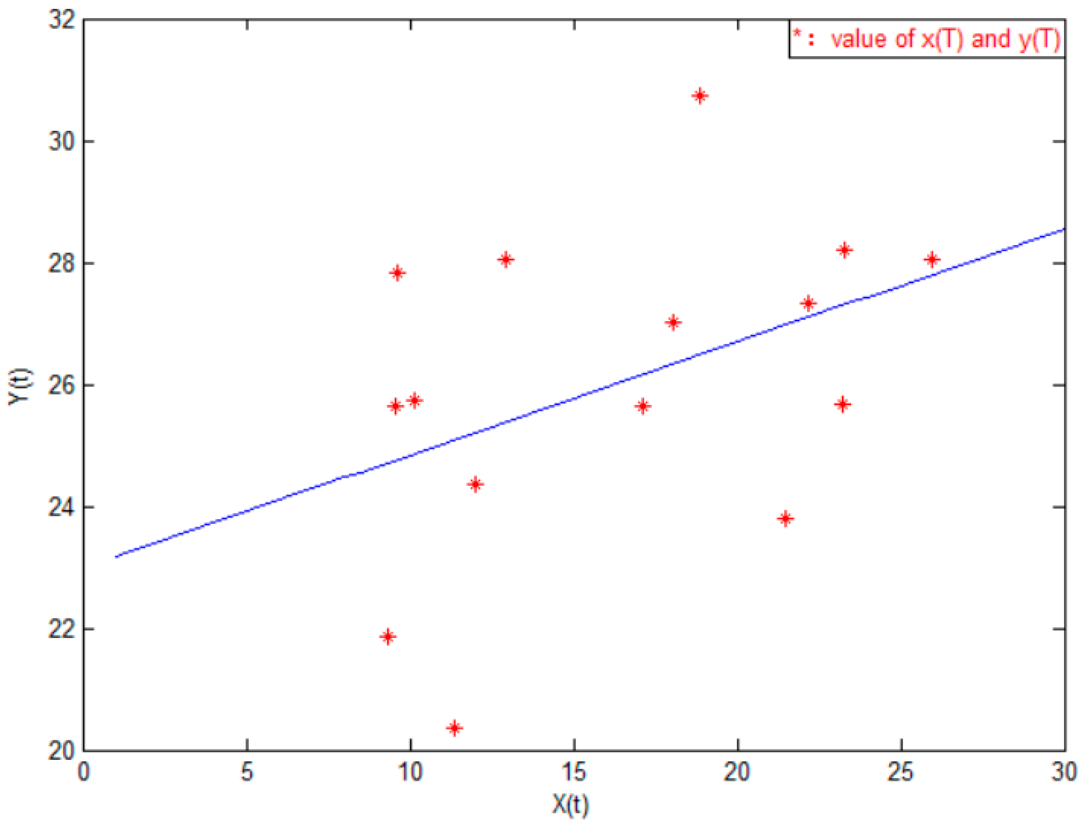
Based on the data of pork prices and the numbers of annual breeding sows, 16 sets of values for X(T) and Y(T) can be calculated by the relationship model between the numbers of new kept gilts and pork prices. The relationship model between the new kept gilts and pork prices is obtained by using the method of least squares to solve the parameters in the model.
Y = 0.185x + 22.986
The effect of regression analysis is shown in Figure 2. X(T) and Y(T) are the variables in Equation (25).
The regression equation was tested for fitness. The correlation modulus of the regression equation was R = 0.42 and the p-value < 0.1.
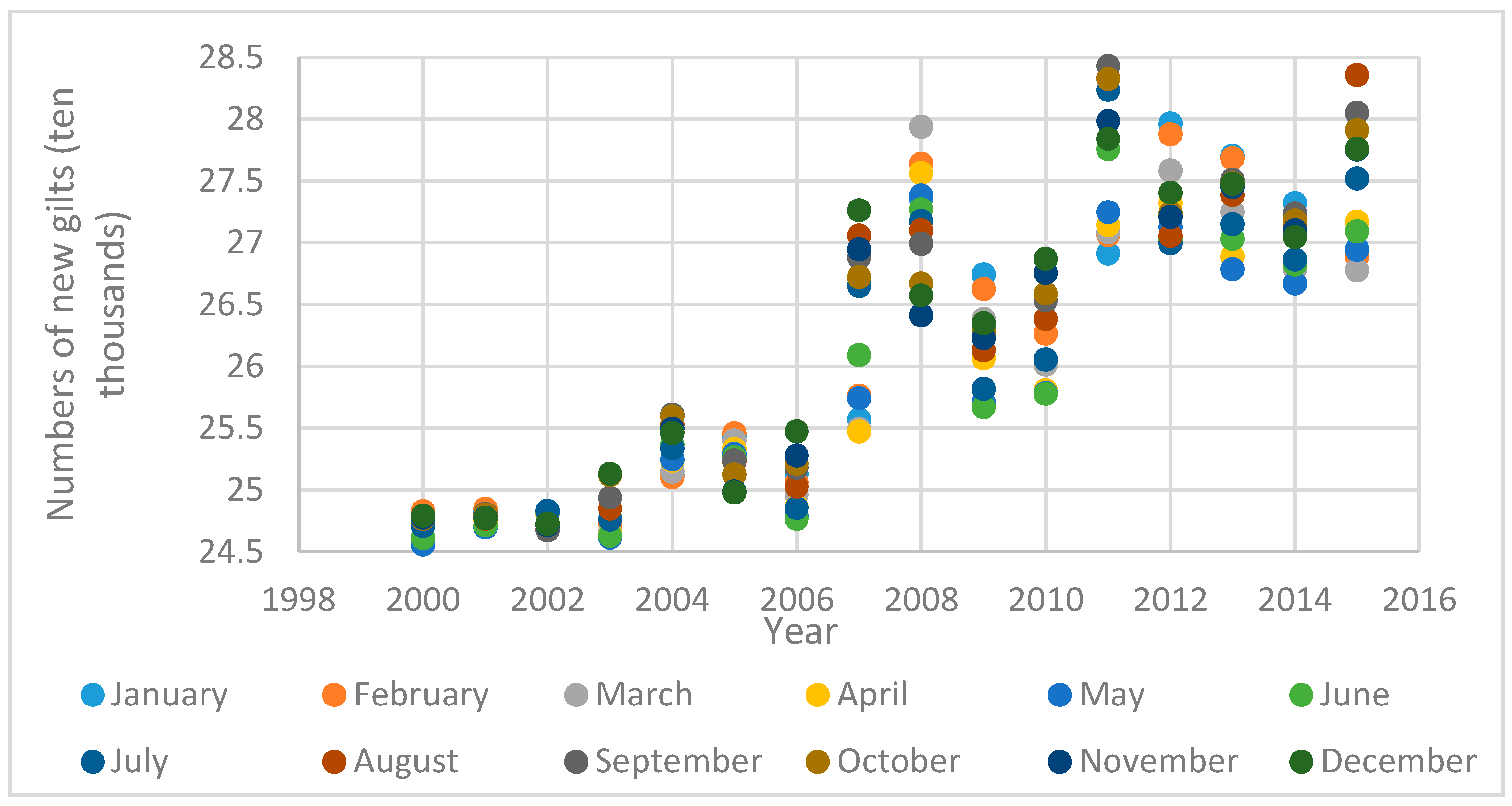
The price of pork from January 2000 to December 2015 in China will be brought into the one-way regression model of new kept gilts and pork prices, and new kept gilts will be obtained from 2000 to 2015 in China. The quantities are shown in Figure 3 below.
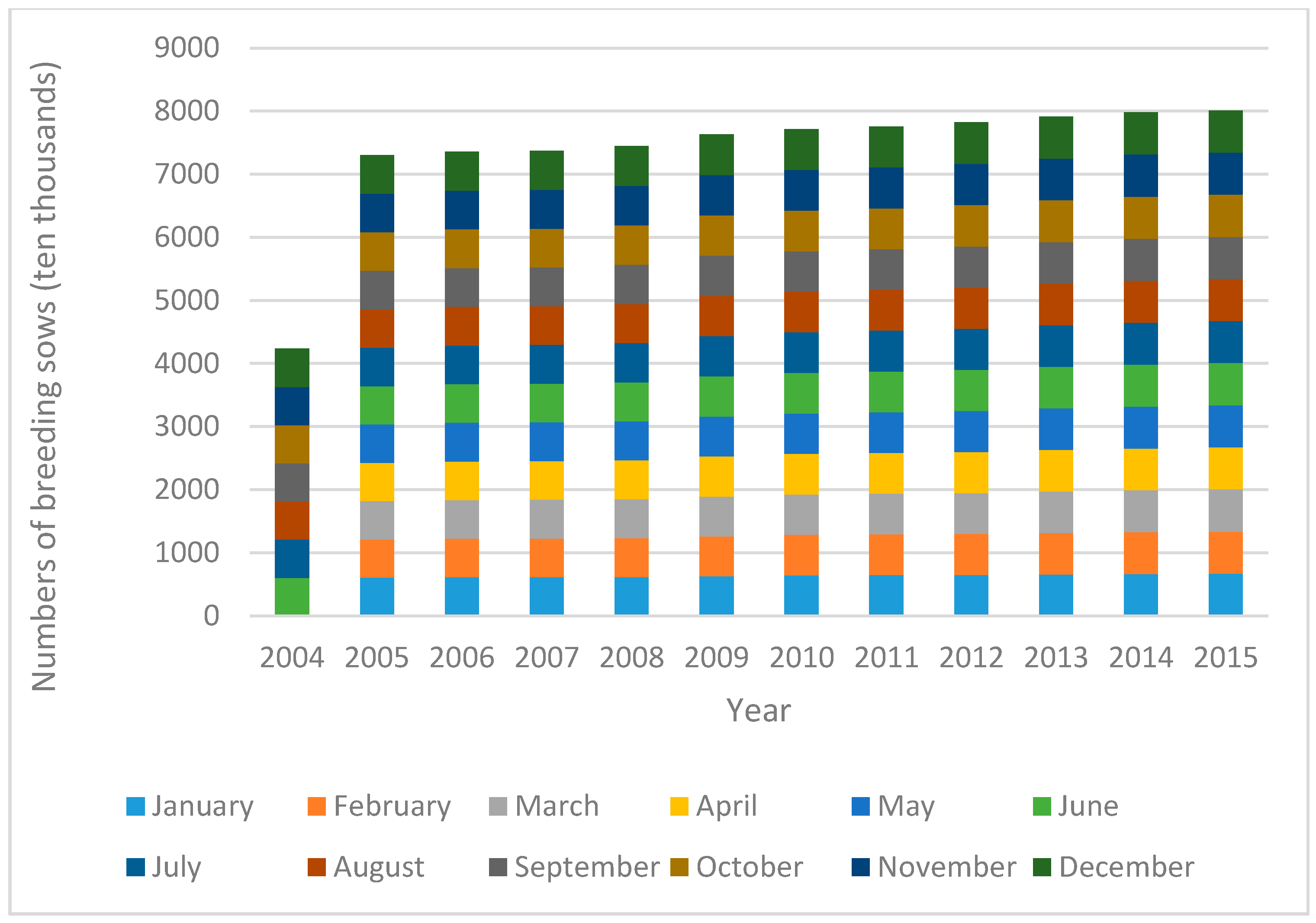
According to the estimated value of the new gilts and the recursive formula of the number of pigs, the number of breeding sows can be obtained from January 2004 to December 2015, as shown in Figure 4.
According to the China Animal Husbandry and Veterinary Statistical Yearbook, the number of actual stocks of breeding sows at the end of 2004 was 566 million. According to the one-way regression equation and the recursive formula, the estimated stock of sows at the end of 2004 was 606 million. The relative error from the actual statistics is 6.4662%. The number of breeding sows in each month of December 2004 was corrected by the number of deviations, and the number of breeding sows in 2004 was 566 million. If December 2004 is the base month of the year, according to the pig group transfer model, the stocks of the breeding sows in the next month can be predicted and compared with the actual statistics. The results are shown in Table 1. In Table 1, relative error refers to the value obtained by multiplying the ratio of the absolute error caused by the measurement to the measured (conventional) true value by 100%, which is expressed as a percentage.
Averaging the number of the deviation is used to obtain an average error of 0.0332 for the estimation of the number of breeding sows. The deviation is small, so the estimation method for the transfer of sows by month is reliable. This method can be used to predict the breeding sow population in the next month.
3.2.2. The Estimation of Initial Pig Population State
This study used 2015 as the base year to forecast the supply of pork in China in the future. Before the prediction, the reliability of the method that estimates the initial pig population state should be verified. After that, this method can be used to estimate the initial state of the population.
➀ Verify the reliability of the initial state estimation method for the population. Take the estimation method of the initial state of the hog population as an example. According to the estimates of the newly retained gilts in China from 2000 to 2015, the estimation of the initial state of the pigs was used to estimate the distribution of the number of pigs per month from 2006 to 2015, and comparing with The Statistical Yearbook of Chinese Animal Husbandry Veterinary shows the comparison of the number of pigs at the end of the year. The analysis results are shown in Table 2.
The deviation and averaging are used to obtain an average error of 0.0368 for the estimation of the number of slaughter pigs. The deviation is small, so the estimation method for the transfer of sows by month is reliable. This method can be used to predict the slaughter pig population in the next month.
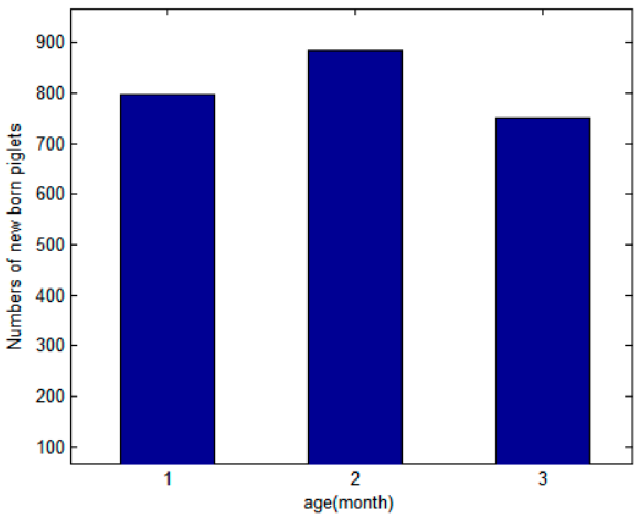
➁ The initial state of the population is estimated, including the initial state of the new born piglets, the sow population, the boar population, and the slaughter pig population. Due to the latest data of the current statistical yearbook to the breeding sows in 2015, this article takes December 2015 as the base year and regards the number of populations as the initial state of the pigs in China; then, the supply of pork in the future will be predicted. We substituted the data of breeding sows into the initial state estimation model; then, the initial state value of new born piglets can be calculated (Figure 5).
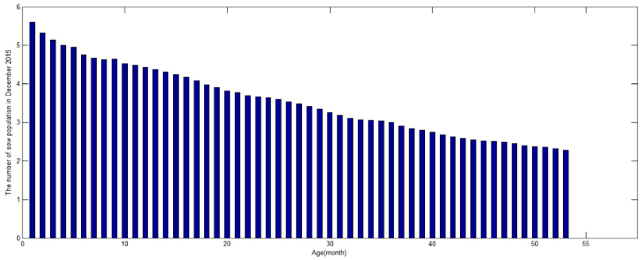
Table 1 indicates that the amount of breeding sows that were stocked in 2015 was 622.186 million. By consulting the China Animal Husbandry and Veterinary Statistical Yearbook, the number of stocks of breeding sows in 2015 was 569 million heads, and the deviation is 0.0935. The number of deviations was used to correct the number of sows in each month of December 2015, and the total number of breeding sows in 2015 was 622.186 million. The adjusted distribution of sows at each month is shown in Figure 6, and the distribution of boar population at each month is shown in Figure 7.
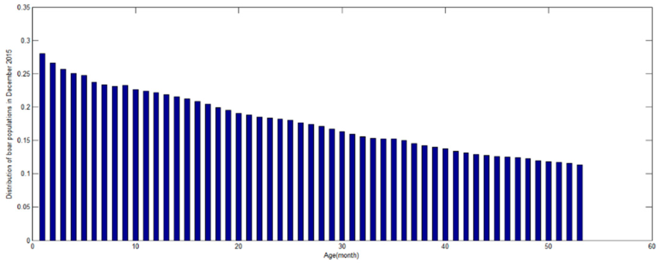
According to the breeding ratio of sows and boars, the distribution of the boar populations in December 2015 was obtained, as shown in Figure 8.
3.2.3. Predict the Distribution of Pig Population in China in the Future
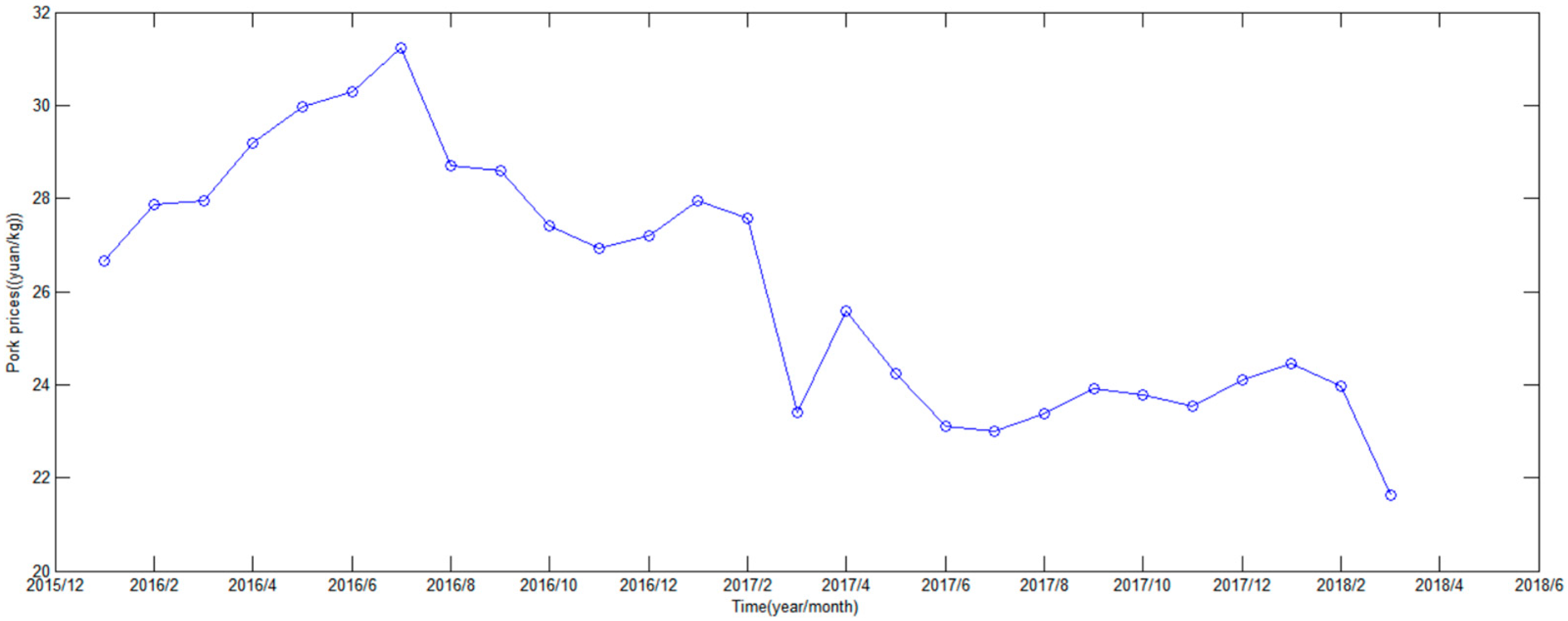
First, the pork prices for each month of China in 2016–2018 are obtained, as shown in Figure 9.
According to the future pork price data, the estimated model of the new gilts for each month is used to calculate the number of new gilts in the future, as shown in Table 3.
Based on the initial state data of the pig population in China in December 2015 and the data of the new gilts, the pig population recursive model was used to obtain the number of breeding sows per month in 2016–2018 which is in the Table 4.
Since the initial state of the slaughter pigs will be released after reaching 6 months of age, the number of slaughter pigs from January 2016 to May 2016 can be obtained according to the initial state of the slaughter pig population in December 2016 in Table 5. In addition, the ability to breed sows in the initial state will breed new born piglets, will experience new kept gilts, boars, and small pigs, and will be released at the end of June. In summary, the number of slaughter pigs in each month from 2016 to 2018 can be calculated by using the recursive model of pig population.
The statistical bulletin of the National Economic and Social Development of China shows that the number of finishing pigs in China in 2016 was 69,254,000, and the number of finishing pigs in 2017 was 65,791,000. According to Table 5 the predicted value of the number of finishing pigs in 2016 was 64,974,955, with an error of 0.0618, and the prediction accuracy is 93.82%. Meanwhile, the value in 2017 is 69,590,558 with an error of 0.0578, and the prediction accuracy is 94.22%.
3.2.4. The Prediction of the Pig Population Index in China in 2017
Based on the above formula for the population index, taking December 2017 as an example, the pig population statistics for December 2017 are calculated as follows:
➀ Year-end stock of breeding sows:
➁ Year-end stock of all pigs:
➂ Column volume of pigs in the current year:
➃ Pork production in the current year:
➄ Number of sows per month at time t December, 2016:
Number of new kept gilts:
Number of replacement sows:
In formula, is the maximum age of replacement sows, and is the minimum age of able to breeding sows, too. is the minimum age of replacement sows.
The number of able sows is as follows:
In this formula, is the maximum month of age of the breeding sows.
The total number of sows is as follows:
➅ Number of boars per month at time t
The number of new kept boars is as follows:
16.962795 ten thousand heads).
The number of replacement boars is as follows:
In this formula, is the age of the piglet when it grows to be a replacement boar, and is the maximum month of age of the replacement boars, that is the minimum month of age of the breeding boar.
The number of breeding boars is as follows:
In formula, is the maximum month of age of the breeding boars.
The number of boars is as follows:
➆ The number of boars at time t.
The number of young pork pigs is as follows:
The number of little nursery pork pigs is as follows:
In this formula, is the age of the piglet when it grows to be a nursery slaughter pig, and is the maximum month of age of the nursery slaughter pigs.
The number of growing slaughter pigs is as follows:
In this formula, is the maximum month of age of the growing slaughter pigs.
The number of fattening slaughter pigs is as follows:
In this formula, is the age of the fattening pork pigs when they grow to finishing pigs.
The number of finishing pigs is as follows:
The total number of slaughter pigs is as follows:
If the average amount of meat produced after slaughtering a pig is c, then the supply of pork at time t is as follows:
➇ Total number of pigs at time t
4. Conclusions
In the fitting stage, the relative error of the estimation of the breeding sows is 0.0332, and the relative error of the initial population estimation is 0.0368. In the prediction stage, the prediction relative error of the number of slaughtered fattened hogs was 0.0618 and 0.0578, and the pig population index in China in the future was predicted. The result shows that according to the prediction accuracy, the prediction model of the pig population based on the population prediction model has higher prediction precision and good prediction effect. According to the viewpoint of modeling, the prediction model of the pig population based on the population prediction model is the effective angle of the research on the prediction of the number of the pig population. The prediction model can reflect the variation of the pig population and related index every month in the future and has obvious advantages over the existing prediction models, which can only predict the annual data. This forecasting model can also make pig farmers manage and control their pig population better. Reasonable breeding can not only make farmers’ input and output symmetrical and reduce farmers’ losses, but it can also reduce the fluctuation of pork price and balance the development of the national economy.
This study not only helps hog breeders make corresponding decisions and plans in a timely manner, but it also provides a reference for the governments at all levels to formulate relevant institutional policies. Of course, there is still a lot to be discussed in this article. For example, it needs to be considered whether there is a more optimized estimation method to estimate the initial state of the pig population. In order to establish the prediction model of the pig population more accurately, other related factors also need to be discussed such as diseases, African swine fever, monthly or seasonal variations of average daily weight gain (growth), fertility, mortality, and so on.
Author Contributions
F.Z., F.W. 1 (Fulin Wang), F.W. 2 (Fulin Wang) worked collectively. F.Z. conceived and designed the study with the support of F.W. 1 (Fulin Wang), F.W. 2 (Fulin Wang) gave constructive suggestions for the idea and the writing. All the co-authors drafted and revised the article together. All authors have read and agreed to the published version of the manuscript.
Funding
This research was funded by Heilongjiang philosophy and social sciences research and planning project “Research on the construction path and innovation platform of agricultural innovation system in Heilongjiang Province” (Project No. 18GLC205).
Conflicts of Interest
The authors declare no conflict of interest.
References
- Zheng, L.; Duan, D.M.; Lu, F.B.; Xu, W.; Wang, S.Y. Integration forecast of Chinese pork consumption demand-empirical based on Arima var and Vec models. Syst. Eng. Theory Pract. 2013, 33, 918–925. [Google Scholar]
- Liu, Y.; Duan, Q.; Wang, D.; Zhang, Z.; Liu, C. Prediction for hog prices based on similar sub-series search and support vector regression. Comput. Electron. Agric. 2019, 157, 581–588. [Google Scholar] [CrossRef]
- Sun, J. Pork price forecast based on breeding sow stocks and hog-grain price ratio. Trans. Chin. Soc. Agric. Eng. 2013, 29, 1–6. [Google Scholar]
- Tao, X.; Chong, L.I.; Yukun, B. An improved EEMD-based hybrid approach for the short-term forecasting of hog price in China. Agric. Econ. 2017, 63, 136–148. [Google Scholar] [CrossRef] [Green Version]
- Zhou, D.; Yu, X.; Herzfeld, T. Dynamic food demand in urban China. China Agric. Econ. Rev. 2015, 7, 27–44. [Google Scholar] [CrossRef] [Green Version]
- Trujillo-Barrera, A.; Garcia, P.; Mallory, M.L. Short-term price density forecasts in the lean hog futures market. Eur. Rev. Agric. Econ. 2017, 45, 121–142. [Google Scholar] [CrossRef]
- Jaile-Benitez, J.M.; Ferrer-Comalat, J.C.; Linares-Mustarós, S. Determining the influence variables in the pork price, based on expert systems. Sci. Methods Treat. Uncertain. Soc. Sci. 2015, 377, 81–92. [Google Scholar]
- Wu, H.; Qi, Y.; Chen, D. A dynamic analysis of influencing factors in price fluctuation of live pigs-based on statistical data in Sichuan province of China. Asian Soc. Sci. 2012, 8, 256. [Google Scholar] [CrossRef] [Green Version]
- Jia, W.; Yang, Y.; Qin, F. The study on China’s pork industry chain price transmission mechanism: Based on province comparison. Stat. Inf. Forum 2013, 3, 49–55. [Google Scholar]
- Zhou, D.; Dieter, K. Price transmission in hog and feed markets of china. J. Integr. Agric. 2015, 6, 1122–1129. [Google Scholar] [CrossRef]
- Jumah, A.; Kunst, R.M. Seasonal prediction of European cereal prices: Good forecasts using bad models? J. Forecast. 2008, 27, 391–406. [Google Scholar] [CrossRef]
- Han, P.; Wang, P.X.; Tian, M.; Zhang, S.Y.; Liu, J.; Zhu, D. Application of the Arima models in drought forecasting using the standardized precipitation index. Appl. Math. Comput. 2012, 392, 352–358. [Google Scholar]
- Yercan, M.; Adanacioglu, H. An analysis of tomato prices at wholesale level in turkey: An application of sarima model. Custos E Agronegocio 2012, 8, 52–75. [Google Scholar]
- Gan, L.I.; Shi-Wei, X.U.; Zhe-Min, L.I.; Yi-Guo, S.; Xiao-Xia, D. Using quantile regression approach to analyze price movements of agricultural products in China. J. Integr. Agric. 2012, 11, 674–683. [Google Scholar]
- Saengwong, S.; Jatuporn, C.; Roan, S.W. An analysis of Taiwanese livestock prices: Empirical time series approaches. J. Anim. Vet. Adv. 2012, 11, 4340–4346. [Google Scholar]
- Gloria, H. Forecasting pseudo-periodic seasonal patterns in agricultural prices. Agric. Econ. 2012, 43, 531–544. [Google Scholar]
- Wu, L.; Liu, S.; Yang, Y. Grey double exponential smoothing model and its application on pig price forecasting in china. Appl. Soft Comput. 2016, 39, 117–123. [Google Scholar] [CrossRef] [Green Version]
- Tian, F.; Peng, Y. Machine vision system of nondestructive real-time prediction of live-pig meat yield. Trans. Chin. Soc. Agric. Eng. 2016, 32, 230–235. [Google Scholar]
- Zhang, J.H.; Li, Z.M.; Kong, F.T.; Dong, X.X.; Chen, W.; Wang, S.W. Prediction of pork prices based on SVM. In Proceedings of the 2013 World Agricultural Outlook Conference, Beijing, China, 6–7 June 2013; Springer: Berlin/Heidelberg, Germany, 2014; pp. 173–178. [Google Scholar]
- Delgado, C.L.; Rosegrant, M.W.; Steinfeld, H.; Ehui, S.K.; Courbois, C. Livestock to 2020: The next food revolution. Vis. Discuss. Pap. 2001, 30, 27–29. [Google Scholar] [CrossRef] [Green Version]
- Jurknait, N.; Djuric, I. Impact of the Russian trade bans on Lithuanian pork sector. Econstor Open Access Artic. 2018, 40, 481–491. [Google Scholar] [CrossRef]
- Meng, Z.; Nan, Z. Lean meat percentage prediction of pig carcass based on radial basis function neural network. J. Agric. Mech. Res. 2017, 6, 38. [Google Scholar]
- Lumogdang, C.F.D.; Wata, M.G.; Loyola, S.J.S.; Angelia, R.E.; Angelia, H.L.P. Supervised Machine Learning Approach for Pork Meat Freshness Identification. In Proceedings of the International Conference on Bioinformatics Research and Applications, Seoul, Korea, 19–21 June 2019; pp. 1–6. [Google Scholar]
- Shih, M.L.; Huang, B.W.; Chiu, N.H.; Chiu, C.; Hu, W.Y. Farm price prediction using case-based reasoning approach—A case of broiler industry in Taiwan. Comput. Electron. Agric. 2009, 66, 70–75. [Google Scholar] [CrossRef]
- Ribeiro, C.O.; Oliveira, S.M. A hybrid commodity price-forecasting model applied to the sugar–alcohol sector. Aust. J. Agric. Resour. Econ. 2011, 55, 180–198. [Google Scholar] [CrossRef]
- Jha, G.K.; Sinha, K. Time-delay neural networks for time series prediction: An application to the monthly wholesale price of oilseeds in India. Neural Comput. Appl. 2014, 24, 563–571. [Google Scholar] [CrossRef]
- Xin, S.; Yi, W.; Duan, S.; Ma, J.H. Detecting chaos from agricultural product price time series. Entropy 2014, 16, 6415–6433. [Google Scholar]
- Liu, T.H.; Li, Z.; Teng, G. Prediction of pig weight based on radical basis function neural network. J. Agric. Mach. 2013, 44, 245–249. [Google Scholar]
- Li, Z.; Xu, S.; Cui, L.; Li, G.; Dong, X.; Wu, Z. The Short-Term Forecast Model of Pork Price Based on CNN-GA. Trans. Tech. Publ. 2013, 628, 350–358. [Google Scholar] [CrossRef]
- Zou, P.; Yang, J.; Fu, J.; Liu, G.; Li, D. Artificial neural network and time series models for predicting soil salt and water content. Agric. Water Manag. 2010, 97, 2009–2019. [Google Scholar] [CrossRef]
- Jang, I.; Lee, S.Y.; Choe, Y.C. Weighted sampling method for improving performance prediction: The case of pig management system. Adv. Sci. Technol. Lett. 2015, 95, 73–77. [Google Scholar] [CrossRef] [Green Version]
- Piewthongngam, K.; Vijitnopparat, P.; Pathumnakul, S.; Chumpatong, S.; Duangjinda, M. System dynamics modelling of an integrated pig production supply chain. Biosyst. Eng. 2014, 127, 24–40. [Google Scholar] [CrossRef]
- Xu, B.; Shi, L.; Liu, Y. Prediction and empirical study of pig price in China. Agric. Econ. Issues 2014, 35, 25–32. (In Chinese) [Google Scholar]
- Zhan, L. Regularity waveform, cause and control of pig price time series. Agric. Mod. Res. 2014, 35, 25–28. (In Chinese) [Google Scholar]
- Song, J. Population Prediction and Population Control; People’s Publishing: Beijing, China, 1982. [Google Scholar]
- Zawadzka, D. The history of research on the “pig cycle”. Probl. Agric. Econ. Zagadnienia Ekonomiki Rolnej 2010, 1, 208–214. [Google Scholar]
Figure 1.
Schematic diagram of the pig population defined in the present study.

Figure 2.
Regression analysis graph of X(T) and Y(T).

Figure 3.
Estimated number of new gilts from 2000 to 2015.

Figure 4.
Estimated number of breeding sows per month from 2004 to 2015.

Figure 5.
Number of new born piglets in December 2015.

Figure 6.
The number of the sow population in December 2015.

Figure 7.
Distribution of boar populations in December 2015.

Figure 8.
Distribution of hog populations in December 2015.

Figure 9.
Pork prices for each month from 2016 to 2018.


Table 1.
A comparison table between the predicted and the actual value of the number of breeding sows in 2004–2015.
Table 1.
A comparison table between the predicted and the actual value of the number of breeding sows in 2004–2015.
| Year | Predictive Value (Ten Thousand) | Actual Value (Ten Thousand) | Relative Error |
|---|---|---|---|
| 2004 | 566 | 566 | |
| 2005 | 570.9614574 | 589 | 0.030625709 |
| 2006 | 573.4566575 | 570 | 0.006064311 |
| 2007 | 574.9350511 | 523 | 0.099302201 |
| 2008 | 585.8609814 | 587 | 0.001940406 |
| 2009 | 598.6894485 | 595 | 0.006200754 |
| 2010 | 603.0519213 | 585 | 0.030857985 |
| 2011 | 605.5471426 | 591 | 0.024614455 |
| 2012 | 613.1236142 | 604 | 0.015105322 |
| 2013 | 618.7693569 | 613 | 0.009411675 |
| 2014 | 624.2275925 | 596 | 0.047361732 |
| 2015 | 622.1858153 | 569 | 0.093472435 |
Table 2.
A comparison table between the predicted and the actual value of the number of finishing pigs in each year.
Table 2.
A comparison table between the predicted and the actual value of the number of finishing pigs in each year.
| Year | Predictive Value (Ten Thousand) | Actual Value (Ten Thousand) | Relative Error |
|---|---|---|---|
| 2006 | 7105.02 | 6780.717945 | 0.047827097 |
| 2007 | 7471.41 | 6804.190631 | 0.098060064 |
| 2008 | 6360.7 | 6809.446693 | 0.06590061 |
| 2009 | 6431.4 | 6961.360612 | 0.076128884 |
| 2010 | 6915.5 | 7108.225114 | 0.027112973 |
| 2011 | 7178.28 | 7149.174708 | 0.00407114 |
| 2012 | 7002.6 | 7180.25797 | 0.024742561 |
| 2013 | 7170.7 | 7276.110933 | 0.014487263 |
| 2014 | 7314.1 | 7344.67785 | 0.004163266 |
| 2015 | 7445 | 7404.611788 | 0.005454467 |
Table 3.
The number of new gilts in each month in 2016–2018.
| Time | Number (Ten Thousand) | Time | Number (Ten Thousand) | Time | Number (Ten Thousand) |
|---|---|---|---|---|---|
| January 2016 | 27.9298 | October 2016 | 28.0708 | July 2017 | 27.2512 |
| February 2016 | 28.1523 | November 2016 | 27.9799 | August 2017 | 27.3216 |
| March 2016 | 28.1672 | December 2016 | 28.0318 | September 2017 | 27.4218 |
| April 2016 | 28.4008 | January 2017 | 28.1690 | October 2017 | 27.3939 |
| May 2016 | 28.5436 | February 2017 | 28.0986 | November 2017 | 27.3531 |
| June 2016 | 28.6029 | March 2017 | 27.3272 | December 2017 | 27.4570 |
| July 2016 | 28.7791 | April 2017 | 27.7314 | January 2018 | 27.5219 |
| August 2016 | 28.3081 | May 2017 | 27.4792 | February 2018 | 27.4329 |
| September 2016 | 28.2896 | June 2017 | 27.2716 | March 2018 | 26.9971 |
Table 4.
The number of breeding sows that can be used in each month in 2016–2018.
| Time | Number (Ten Thousand) | Time | Number (Ten Thousand) | Time | Number (Ten Thousand) |
|---|---|---|---|---|---|
| January 2016 | 665.2360 | October 2016 | 665.3340 | July 2017 | 672.4522 |
| February 2016 | 664.3963 | November 2016 | 665.8391 | August 2017 | 673.1802 |
| March 2016 | 663.9295 | December 2016 | 666.4881 | September 2017 | 673.8585 |
| April 2016 | 663.4213 | January 2017 | 667.2831 | October 2017 | 674.4909 |
| May 2016 | 663.0983 | February 2017 | 668.0141 | November 2017 | 675.0584 |
| June 2016 | 663.0819 | March 2017 | 668.9140 | December 2017 | 675.6828 |
| July 2016 | 663.7822 | April 2017 | 669.9261 | January 2018 | 676.1457 |
| August 2016 | 664.3333 | May 2017 | 670.8922 | February 2018 | 675.9240 |
| September 2016 | 664.8637 | June 2017 | 671.8684 | March 2018 | 676.0462 |
Table 5.
Prediction of the number of finishing pigs in each month in 2016–2018.
| Time | Number (Ten Thousand) | Time | Number (Ten Thousand) | Time | Number (Ten Thousand) |
|---|---|---|---|---|---|
| January 2016 | 579.3772 | October 2016 | 575.9535917 | July 2017 | 579.6922849 |
| February 2016 | 579.65269 | November 2016 | 575.5439568 | August 2017 | 580.9896057 |
| March 2016 | 579.7294325 | December 2016 | 575.4801702 | September 2017 | 581.4689223 |
| April 2016 | 579.7225285 | January 2018 | 576.3562409 | October 2017 | 582.5915294 |
| May 2016 | 597.6500583 | February 2017 | 576.8695025 | November 2017 | 583.6358593 |
| June 2016 | 122.7583752 | March 2017 | 577.5293108 | December 2017 | 584.5347175 |
| July 2016 | 577.9820714 | April 2017 | 578.0292742 | January 2018 | 585.0040278 |
| August 2016 | 577.0397165 | May 2017 | 578.4427404 | February 2018 | 585.5790734 |
| September 2016 | 576.6056677 | June 2017 | 578.9158294 | March 2018 | 586.2149126 |
Publisher’s Note: MDPI stays neutral with regard to jurisdictional claims in published maps and institutional affiliations. |
© 2021 by the authors. Licensee MDPI, Basel, Switzerland. This article is an open access article distributed under the terms and conditions of the Creative Commons Attribution (CC BY) license (http://creativecommons.org/licenses/by/4.0/).
Share and Cite
MDPI and ACS Style
Zhang, F.; Wang, F.; Wang, F. Forecasting Model and Related Index of Pig Population in China. Symmetry 2021, 13, 114. https://doi.org/10.3390/sym13010114
AMA Style
Zhang F, Wang F, Wang F. Forecasting Model and Related Index of Pig Population in China. Symmetry. 2021; 13(1):114. https://doi.org/10.3390/sym13010114
Chicago/Turabian StyleZhang, Fan, Fulin Wang, and Fulin Wang. 2021. "Forecasting Model and Related Index of Pig Population in China" Symmetry 13, no. 1: 114. https://doi.org/10.3390/sym13010114
Note that from the first issue of 2016, this journal uses article numbers instead of page numbers. See further details here.