Eliminate the Queuing Time in the New Suez Canal: Predicting Adjustment on Ships’ Arrival Time under Optimal Non-Queuing Toll Scheme

Abstract

In 2016, the construction of the New Suez Canal was completed, enabling most large-size vessels to pass through and causing more ships to queue into the canal. As the queueing problem at the entrance of the canal was anticipated to be serious, an optimal non-queueing toll scheme was previously established to eliminate the queueing phenomenon at the anchorage of the canal. However, no information about each ship’s arrival time adjustment under the optimal non-queueing toll scheme is available from the previous literature. To solve this problem, we derive a series of mathematical formulae for each ship’s arrival time, length of queuing time and entry time before, and after, implementing the optimal non-queueing toll scheme. The arrival time adjustments, which enable ships to enter the canal without queueing, could then be obtained. These results enable the Suez Canal authorities to draw up the ship’s arrival timetable under the optimal non-queueing toll scheme, so that the captain could follow to enter the canal. The above information that we provide would be conducive to the management decision for the canal authorities to implement such a toll scheme. Once a tolled ship could enter the canal at the scheduled time without queueing, the ship owner could accurately control the sailing schedule, and the use of the ship could be more efficient.

1. Introduction

The Suez Canal had only one waterway, and some large tankers (such as the Very Large Crude Carrier, 160,000~320,000 DWT) were not allowed to enter the canal because of size limitations (Suez Canal max, 130,000~200,000 DWT) before the expansion construction. To address these shortcomings, in addition to widening and deepening the original 37-km waterway, the New Suez Canal has added a 35-km parallel waterway that enables ships to sail in both directions simultaneously. After the completion of the construction expansion in 2016, most large-size ships have been allowed to pass through the canal. According to the Suez Canal Authority, the number of ships that passed through the canal in 2019 was 18,880, which was significantly higher than 16,833 ships in 2016. Furthermore, according to the first item of Project Returns and Outcome in the Official Suez Canal Website (http://0rz.tw/9Mlg3), the Egyptian government predicts that the daily number of ships that will enter the canal in 2023 will be twice that in 2016. The aforementioned data indicates that the use of the New Suez Canal has continued to increase after the expansion. While the capacity of the New Suez Canal has increased after the construction, long queues at the anchorage of the canal continue to be a serious issue because the large-size ships that had been unable to pass before the expansion have now joined the ranks. To solve the current problem of a large number of ships waiting in line to enter the New Suez Canal, a pricing scheme to disperse all ships’ arrival times and eliminate queuing could be introduced as an effective method.

The current Suez Canal charges are the canal operation and maintenance costs incurred when a ship sails through the canal, including pilotage fees, transit expenses, mooring and miscellaneous fees. While the optimal non-queueing toll scheme with continuous changes in the toll amount has been developed by Laih et al. [1] to eliminate the efficiency loss caused by queueing at the canal’s anchorage. Different from the purpose of the current Suez Canal charges of operation and maintenance costs, the optimal non-queueing toll scheme could enhance a canal’s passage efficiency (i.e., zero queueing at the entry of the canal).

In the relevant literature on queueing pricing, Vickrey [2] first determined the optimal variable toll to eliminate auto-commuters’ queueing times spent at a road bottleneck. Since then, many researchers have extended Vickrey’s model to address bottleneck queueing during the morning rush hour. For example, Small [3] derived the values of the time spent waiting in the queue as well as the penalties of arriving at the workplace before and after the official starting time under the Vickrey’s model. Such derived values were $6.40, $3.90, and $15.21 per hour, respectively, for 572 homogeneous motorists in the San Francisco Bay Area. Cohen [4] applied Vickrey’s model to simulate changes in the welfare effects for higher- and lower-income commuters under the implementation of the optimal non-queueing toll. The study pointed out that both groups of motorists never lost and gained the welfare effects after the implementation of the toll scheme. In addition, Braid [5], Arnott et al. [6] and Laih [7,8] also applied Vickrey’s model to derive the optimal non-queueing toll and alternative tolls to eliminate and reduce the total queueing time at a commuting road bottleneck. Additionally, Small [9] assessed and interpreted the bottleneck model, stating that it will become more suitable for practice and application if some topics were incorporated into it to correspond to reality, such as travellers with heterogeneous values of time and scheduling preferences, networks instead of a single bottleneck, changes in residential locations, the lack of stochastic information, hyper-congestion and others.

Vickrey’s pricing model was also applied to maritime transportation. The first type of application is the development of a pricing model for ships queueing for vacant berths at a busy port. Laih and Chen [10] first devised an optimal non-queueing toll scheme for container ships queueing for a single berth at a busy port. In addition, Laih and Sun [11] deduced an optimal non-queueing toll scheme for bulk carriers queueing for multiple berths. After implementing the optimal non-queueing toll schemes, the queueing times of all ships at the anchorage zone could be eliminated. Furthermore, Sun et al. [12] proposed the optimal non-queueing toll scheme for trampers queueing for shared-use berths, because most bulk carrier berths are shareable in practice. The second type of application is the development of a pricing model for ships queueing to enter a busy canal. Laih et al. (2015) first established a pricing model to derive the optimal non-queueing toll scheme for the New Suez Canal. The implementation of this toll scheme could be anticipated to eliminate the inefficiency of queueing for entry into this canal.

It is noted that Laih et al. [1] have constructed the optimal non-queueing toll scheme for the New Suez Canal to eliminate the total queuing time of all ships waiting for entry into the canal and achieve the efficient use of the canal. However, no information regarding each ship’s arrival time adjustment from the no-toll to the tolled case is available from the previous study for management decision and practical application. To solve this problem, we derive a series of mathematical formulae for each ship’s arrival time, length of queuing time and entry time before and after implementing the optimal non-queueing toll scheme. Then arrival time adjustments, which enable all ships to enter the New Suez Canal without queuing, could be obtained. According to our mathematical formulae, the canal authority could announce the timetable of arrival that each ship must comply with and the amount of optimal non-queueing toll that each ship should pay during the canal’s operating hours. The above information that we provide would be conducive to the implementation of an electronic canal pricing system. Such effective management could eliminate the issues associated with ships waiting in line to enter the canal. From the shipowner’s perspective, the ship could simply follow the canal authority’s instructions to enter the canal at the scheduled time without queuing at the anchorage zone. This would enable the shipowner precisely control the sailing schedule to cross the canal and lead to the significant reduction of fuel consumption of ships.

The main academic contribution and practical implication of this paper are:

(1)

The purpose of this article is to show how each ship could adjust their original arrival time to enter the New Suez Canal without queueing once the optimal non-queueing toll scheme was implemented. We will solve this problem by presenting an analytic mathematical model to explain how ships could adjust their anchorage arrival times from the no-toll to the tolled case. This is a crucial information to forecast each tolled ship’s arrival decision that related studies have never discussed before.

(2)

Based on the above information, the canal authority could implement an electronic canal pricing system with the timetable of arrival that each ship must comply with and the amount of optimal non-queueing toll that each ship should pay during the canal’s operating hours. Such an effective management could eliminate the phenomenon of ships waiting in line to enter the canal.

(3)

From the shipowner’s perspective, the ship could enter the New Suez Canal smoothly (without queueing) by following the announced timetable, so as not to cause the loss due to delay in sailing schedule. The captain could simply follow the instruction to enter the canal at the scheduled time without having to stop engines and queueing for the entry under the optimal non-queueing toll scheme.

(4)

Avoiding stop-and-go in the canal’s anchorage zone under the optimal non-queueing toll scheme would not only greatly reduce the fuel consumption of ships, but also could reduce the risk of ship manipulation (e.g., accidents such as ship collisions or the anchor chain entanglement incidents in the canal’s anchorage zone) that may occur when a ship enters and exits an anchorage zone with limited space.

The rest of this article is organized as follows. Section 2 surveys the relevant literature regarding the derivation of the no-toll equilibrium and the optimal non-queueing toll scheme for the New Suez Canal. Section 3 provides a methodology that uses mathematical formulae to show each ship’s arrival time adjustment from the no-toll to the tolled case, which would enable all ships to enter the New Suez Canal without queueing. Section 4 performs a numerical analysis that simulates this methodology based on the latest data and statistics for the year 2019. Section 5 provides the conclusion of this paper.

2. Review of No-Toll Equilibrium and Optimal Non-Queueing Toll Scheme

In this section, we review how the no-toll equilibrium and the optimal non-queueing toll scheme were derived for queueing ships at the anchorage of the New Suez Canal. The basic assumptions of this model are summarized as follows:

• All ships have to be queued to enter the New Suez Canal. Queueing occurs only at the designated anchorage of the canal because of its capacity restriction.
• Only a fixed number of queueing ships are allowed to enter the canal per day.
• The cost function for each ship include the queueing time cost and the time-early cost or time-late cost caused by queueing.
• All ships determine their arrival times at the anchorage of the New Suez Canal. Therefore, the cost per ship is the function of its arrival time.

In general, there are three possible types of arrival pattern at the New Suez Canal’s anchorage, namely, time-early, on-time and time-late scheduling.

Table 1. The cost function for a ship with each of the three types of arrival pattern.

Scheduling	Time Period	$\mathbf{The}\mathbf{Cost}\mathbf{Function}(\mathit{C}(\mathit{t}))$
Time-early	$\begin{array}{l}{t}_q\le t+T_Q(t)<t^{*}\\ (\mathrm{or} t<\tilde{t})\end{array}$	$\begin{array}{ll}C(t)& =\alpha \cdot T_Q(t)+\beta \cdot T_E(t)\\ & =\alpha \cdot T_Q(t)+\beta \cdot [t^{*}-(t+T_Q(t)]\end{array}$
On-time	$\tilde{t}+T_Q(\tilde{t})=t^{*}$	$C(\tilde{t})=\alpha \cdot T_Q(\tilde{t})$
Time-late	$\begin{array}{l}{t}^{*}<t+T_Q(t)\le t_{q^{\prime }}\\ (\mathrm{or} t>\tilde{t})\end{array}$	$\begin{array}{ll}C(t)& =\alpha \cdot T_Q(t)+\gamma \cdot T_L(t)\\ & =\alpha \cdot T_Q(t)+\gamma \cdot [(t+T_Q(t)-t^{*}]\end{array}$

$t$: a ship’s arrival time at the New Suez Canal’s anchorage. $t^{*}$: the latest permitted time (23:00) to enter the New Suez Canal per day. $\tilde{t}$: the time spot at which enables a ship to enter the New Suez Canal at $t^{*}$. $t_q$: the time spot at which queueing begins to build up at the anchorage. $t_{q^{\prime }}$: the time spot at which queueing dissipates at the anchorage. $T_Q(t)$: the length of time spent waiting in the queue at t.$T_E(t)$: the length of time of early entry before $t^{*}$. $T_L(t)$: the length of time of delayed entry after $t^{*}$. $\alpha$: the hourly opportunity cost of $T_Q(t)$. $\beta$: the hourly penalty cost of $T_E(t)$. $\gamma$: the hourly penalty cost of $T_L(t)$. C(t): the cost function per ship.

shows these three schedules as (1) time-early, $t+T_Q(t)<t^{*}$, (2) on-time, $\tilde{t}+T_Q(\tilde{t})=t^{*}$ and (3) time-late, $t+T_Q(t)>t^{*}$. where t means a ship’s arrival time at the New Suez Canal’s anchorage; $t^{*}$ means the latest permitted time (23:00) to enter the New Suez Canal per day; $\tilde{t}$ means the time spot at which enables a ship to enter the New Suez Canal at $t^{*}$; $T_Q(t)$ means the length of time spent waiting in the queue at t. The cost function (C(t)) for a ship due to queueing at the anchorage consists of two parts. One is the opportunity cost of waiting in queue (i.e., queueing time cost), and the other is the penalty cost to a ship that entered the canal earlier or later than the latest permitted entry time ($t^{*}$ = 23:00). As shown in Table 1, we express the cost function, C(t), for a queueing ship with each of the three schedules.

A ship with one of the three arrival patterns will be satisfied with its arrival time (t) in the equilibrium state, and the cost (C(t)) for the ship is its minimum value at this time. Because each ship seeks to minimize the cost, it will reach a stable situation that all ships have the same cost in the equilibrium state. Therefore, the equilibrium condition can be shown as $\frac{dC(t)}{dt}=0$ for all arrival times (t).

Table 2. Derivation of the no-toll equilibrium.

Scheduling	Time Period	$\mathbf{Slope}\mathbf{of}{\mathit{T}}_{\mathit{Q}}(\mathit{t})$	$\mathbf{Equilibrium}\mathbf{Cost}\left({\mathit{C}}^{\mathit{e}}\right)$
Time-early	$\begin{array}{l}{t}_q\le t+T_Q(t)<t^{*}\\ (\mathrm{or}t<\tilde{t})\end{array}$	$\frac{d{T}_Q(t)}{dt}=\frac{\beta }{\alpha -\beta }$	$\begin{array}{ll}C(t_q)& =\alpha \cdot T_Q(t_q)+\beta \cdot T_E(t_q)\\ & =\frac{\beta \cdot \gamma }{\beta +\gamma }\left(\frac{N}{S}\right)=C^e\end{array}$
On-time	$\tilde{t}+T_Q(\tilde{t})=t^{*}$	Nondifferentiable ($\tilde{t}$ is a time spot)	$\begin{array}{ll}C(\tilde{t})& =\alpha \cdot T_Q(\tilde{t})\\ & =\frac{\beta \cdot \gamma }{\beta +\gamma }\left(\frac{N}{S}\right)=C^e\end{array}$
Time-late	$\begin{array}{l}{t}^{*}<t+T_Q(t)\le t_{q^{\prime }}\\ (\mathrm{or} t>\tilde{t})\end{array}$	$\frac{d{T}_Q(t)}{dt}=\frac{-\gamma }{\alpha +\gamma }$	$\begin{array}{ll}C(t_{q^{\prime }})& =\alpha \cdot T_Q(t_{q^{\prime }})+\gamma \cdot T_L(t_{q^{\prime }})\\ & =\frac{\beta \cdot \gamma }{\beta +\gamma }\left(\frac{N}{S}\right)=C^e\end{array}$
$Solving \{\begin{array}{l}{t}_{q^{\prime }}-t_q=\frac{N}{S}\\ \tilde{t}+\frac{\beta }{\alpha -\beta }(\tilde{t}-t_q)=t^{*}\Rightarrow \\ \tilde{t}+\frac{-\gamma }{\alpha +\gamma }(\tilde{t}-t_{q^{\prime }})=t^{*}\end{array}$$\{\begin{array}{l}{t}_q=t^{*}-\frac{\gamma }{\beta +\gamma }\cdot \left(\frac{N}{S}\right)\\ \tilde{t}=t^{*}-\frac{\beta \gamma }{\alpha (\beta +\gamma )}\cdot \left(\frac{N}{S}\right)\\ t_{q^{\prime }}=t^{*}+\frac{\beta }{\beta +\gamma }\cdot \left(\frac{N}{S}\right)\end{array}$ N: the total number of queueing ships, S: the capacity of the New Suez Canal

shows these equilibrium results for the three types of scheduling. Because $\gamma >\alpha >\beta >0$ is a reasonable order relation in the shipping practice (Laih et al., 2015), the queue increases linearly from $t_q$ to a maximum at $\tilde{t}$ with a positive slope during the time-early scheduling, after which it decreases linearly from $\tilde{t}$ to $t_{q^{\prime }}$ with a negative slope during the time-late scheduling. Clearly, the shape of $T_Q(t)$ may or may not be symmetric around $\tilde{t}$ depending on whether $2(\beta \cdot \gamma )$ is equal to $\alpha (\gamma -\beta )$.

Using these positive and negative slopes of $T_Q(t)$, on-time scheduling can be expressed as $\tilde{t}+\frac{\beta }{\alpha -\beta }(\tilde{t}-t_q)=t^{*}$ and $\tilde{t}+\frac{-\gamma }{\alpha +\gamma }(\tilde{t}-t_{q^{\prime }})=t^{*}$, respectively. In addition, we assume that at the most N ships can enter the canal per day, and the hourly capacity (S) of the canal is fixed; then the length of queueing time period ($t_q-t_{q^{\prime }}$) at the anchorage per day can be obtained as $t_{q^{\prime }}-t_q=\frac{N}{S}$. Solving for these three equations, we obtain three crucial time spots, $t_q$, $\tilde{t}$ and $t_{q^{\prime }}$, as shown at the bottom of Table 2. Because all ships have the same cost in equilibrium, substituting $t_q$, $\tilde{t}$ and $t_{q^{\prime }}$ into their corresponding costs yields the equilibrium cost per ship, $C^e$, as shown by the right side of Table 2. The no-toll equilibrium can be achieved when all ships determine their arrival times at which their costs are all equal to $C^e$. Therefore, all queueing ships are not incentivized to change their arrival times in this situation.

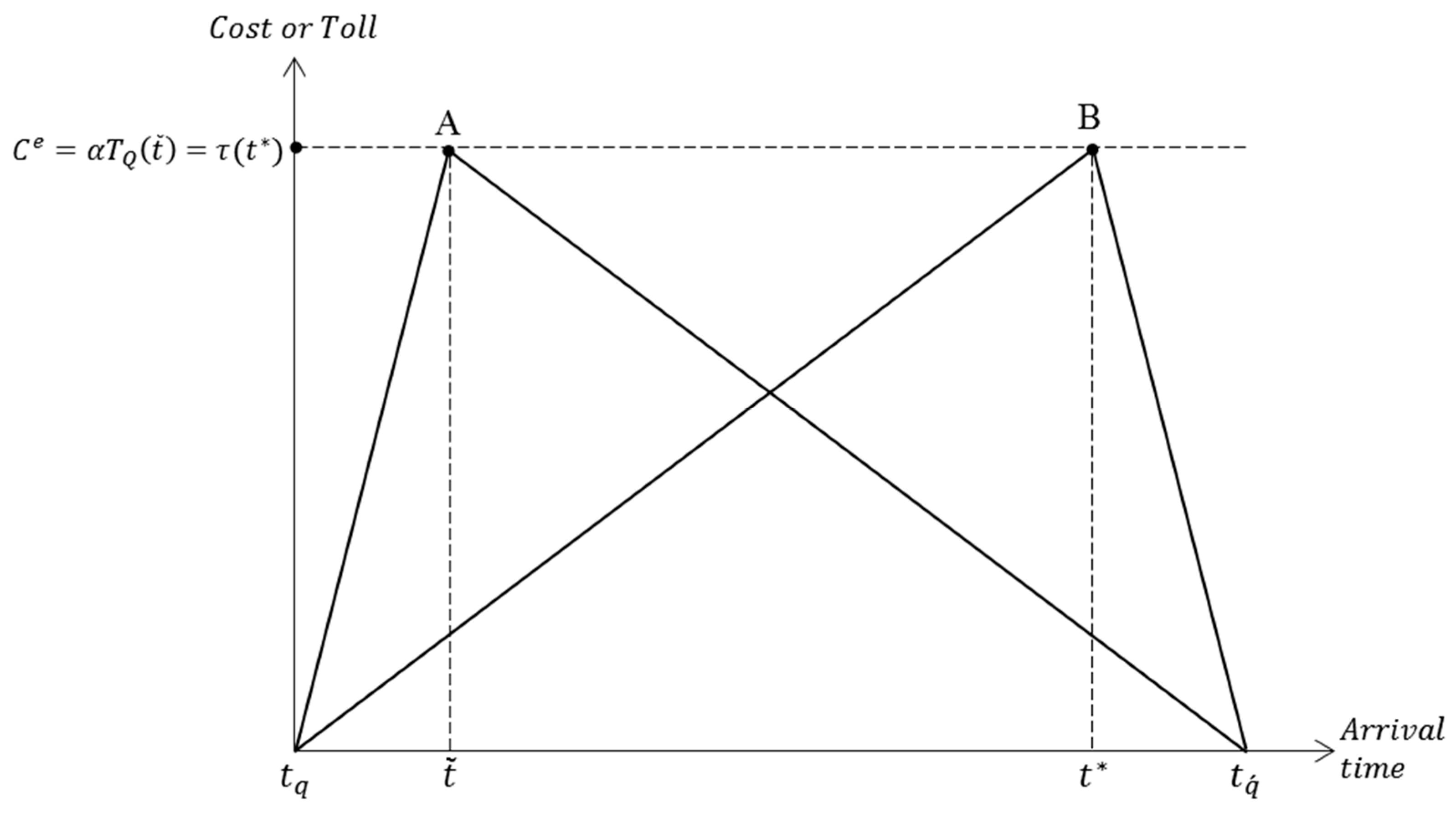
Based on Table 2, The left triangle $t_{q}A{t}_{q^{\prime }}$ in Figure 1 is a schematic of queueing time cost ($\alpha \cdot T_Q(t)$), and the slopes of the left and right sides are $\frac{\alpha \beta }{\alpha -\beta }$ and $\frac{-\alpha \gamma }{\alpha +\gamma }$, respectively. In addition, the triangle apex (point A) represents both the highest queueing time cost ($\alpha \cdot T_Q(\tilde{t})$) and the equilibrium cost ($C^e$).

The optimal non-queueing toll scheme with continuous changes in the toll amount has been developed to eliminate the efficiency loss caused by queueing at the New Suez Canal’s anchorage. To achieve the optimization model, the optimal non-queueing toll ($\tau (t)$) that results in zero queueing (i.e., $T_Q(t)=0$) and under which all ships are no worse off than they would be in the no-toll equilibrium (i.e., $C(t)=C^e$) can be obtained as shown in

Table 3. Derivation of the optimal non-queueing toll scheme.

Scheduling	Tolling Period	The Optimal Non-Queueing Toll $(\mathit{\tau }(\mathit{t}))$
Time-early	$t_q\le t<t^{*}$	$\begin{array}{l}C(t)=\alpha \cdot T_Q(t)+\beta \cdot T_E(t)+\tau (t)=C^e\\ \tau (t)=C^e-\beta \cdot [t^{*}-(t+T_Q(t))]\\ \hspace{1em}\hspace{1em}=C^e-\beta \cdot (t^{*}-t)\end{array}$
On-time	$t^{*}$	$\begin{array}{l}C(t^{*})=\alpha \cdot T_Q(t^{*})+\tau (t^{*})=C^e\\ \tau (t^{*})=C^e\end{array}$
Time-late	$t^{*}<t\le t_{q^{\prime }}$	$\begin{array}{l}C(t)=\alpha \cdot T_Q(t)+\gamma \cdot T_L(t)+\tau (t)=C^e\\ \tau (t)=C^e-\gamma \cdot [(t+T_Q(t))-t^{*}]\\ \hspace{1em}\hspace{1em}=C^e-\gamma \cdot (t-t^{*})\end{array}$

. The highest optimal non-queueing toll is located at the latest time ($t^{*}$) permitted to enter the canal, which is reasonable because ships are willing to pay the highest toll and enter the canal without incurring any time-early or time-late costs. The optimal non-queueing tolls before and after $t^{*}$ are relatively low because of the involvement of time-early, and time-late costs, respectively.

From Table 3, the optimal non-queueing tolls increase linearly from the queue starting time ($t_q$) to a maximum at $t^{*}$ with a positive slope ($\beta$) for time-early scheduling, after which the tolls decrease linearly from $t^{*}$ to the queue ending time ($t_{q^{\prime }}$) with a negative slope ($-\gamma$) for time-late scheduling. Clearly, the optimal non-queueing toll function for time-late scheduling is always steeper than that for time-early scheduling because $\gamma >\beta >0$.

A schematic of the optimal non-queueing toll scheme ($\tau (t)$) is shown in Figure 1 as the triangle $t_{q}B{t}_{q^{\prime }}$ with the slopes $\beta$ and $-\gamma$ on the left and right sides, respectively. In addition, the triangle apex (point B) represents $\tau (t^{*})$. It is clear that the maximum optimal non-queueing toll is identical to the highest queueing time cost in the no-toll equilibrium, that is, $\tau (t^{*})=\alpha \cdot T_Q(\tilde{t})=C^e$.

The advantage of the optimal non-queueing toll scheme is that it could completely eliminate the queuing time of ships in the anchorage zone, so that ships could enter the canal without waiting in line. However, there will be some practical drawbacks once this toll scheme is implemented. First, the optimal non-queueing tolls change continuously, and it may not be easily implemented by the canal authorities because of the complicated tolling mechanism. Second, the canal users cannot choose whether to pay or not; that is, all ships must pay the continuously changing toll for canal passage during the queuing period.

Due to the complicated and variable continuous charging method, the optimal non-queueing toll scheme must be coordinated with the electronic toll collection system (ETCS) for effective implementation. Before implementing ETCS, the canal authorities have to first establish a daily timetable for ships to arrive at the anchorage of the canal and the corresponding amount of charges. These crucial information will be provided by using our mathematical formulae developed in the next Section.

3. Arrival Time Adjustments under the Optimal Non-Queueing Toll Scheme

The optimal non-queueing toll scheme could enhance a canal’s passage efficiency (i.e., zero queueing). However, no information about ships’ arrival time adjustments from the no-toll to the tolled case is available for theoretical improvement, as well as practical references. In this section, we will solve this problem by presenting a methodology to show how ships could adjust their anchorage arrival times from the no-toll to the tolled case. These arrival time adjustments would be conducive to establish the ship’s arrival timetable under the optimal non-queueing toll scheme, so that the captain could follow to enter the canal without queueing. Such an electronic canal pricing system could eliminate the phenomenon of ships waiting in line to enter the New Suez Canal. The following shows the results of group shift and individual movement to illustrate all ships’ arrival time adjustments from the no-toll to the tolled case at the New Suez Canal.

3.1. Group Shift in Arrival Time Period

Computing and comparing different arrival rates between the no-toll and the tolled cases are the first step to realize the changes in ships’ arrival decisions. Arrival rate is defined as the number of arrived ships per hour. Because the number of ships permitted to enter the New Suez Canal corresponds to its capacity (S) throughout the queueing period, and because the marginal arrival rate is $\frac{d(S\cdot T_Q(t))}{dt}$, arrival rates for all queueing ships can therefore be obtained as $S+\frac{d(S\cdot T_Q(t))}{dt}$, for $t_q\le t\le t_{q^{\prime }}$. Accordingly,

Table 4. Arrival rates and total arrivals before and after implementing the optimal non-queueing toll scheme.

Situation	Scheduling	Time Period	Arrival Rate	Total Arrivals
No-toll equilibrium	Time-Early	$t_q\le t<\tilde{t}$	$\begin{array}{l}S+\frac{d(S\cdot T_Q(t))}{dt}\\ =S+\frac{\beta \cdot S}{\alpha -\beta }=\frac{\alpha \cdot S}{\alpha -\beta }\end{array}$	$\begin{array}{l}\frac{\alpha \cdot S}{\alpha -\beta }\cdot (\tilde{t}-t_q)\\ =\frac{\gamma \cdot N}{\beta +\gamma }\end{array}$
	Time-Late	$\tilde{t}<t\le t_{q^{\prime }}$	$\begin{array}{l}S+\frac{d(S\cdot T_Q(t))}{dt}\\ =S-\frac{\gamma \cdot S}{\alpha +\gamma }=\frac{\alpha \cdot S}{\alpha +\gamma }\end{array}$	$\begin{array}{l}\frac{\alpha \cdot S}{\alpha +\gamma }\cdot (t_{q^{\prime }}-\tilde{t})\\ =\frac{\beta \cdot N}{\beta +\gamma }\end{array}$
Optimal non-queueing toll scheme	Time-Early	$t_q\le t<t^{*}$	S	$\begin{array}{l}S\cdot (t^{*}-t_q)\\ =\frac{\gamma \cdot N}{\beta +\gamma }\end{array}$
	Time-Late	$t^{*}<t\le t_{q^{\prime }}$	S	$\begin{array}{l}S\cdot (t_{q^{\prime }}-t^{*})\\ =\frac{\beta \cdot N}{\beta +\gamma }\end{array}$

shows the variation in arrival rates before and after the implementation of the optimal non-queueing toll scheme.

In Table 4, because the slopes of queueing time length $\left(i.e.,\frac{d{T}_Q(t)}{dt}\right)$ for the time-early and time-late schedulings under the no-toll equilibrium are $\frac{\beta }{\alpha -\beta }$ and $\frac{-\gamma }{\alpha +\gamma }$, respectively, arrival rates for these two schedules are equal to $\frac{\alpha \cdot S}{\alpha -\beta }$ and $\frac{\alpha \cdot S}{\alpha +\gamma }$, respectively. The total number of arriving ships can be computed by multiplying the arrival rates and their corresponding time intervals. Subsequently, the total number of arrivals for the time-early and time-late schedules can be obtained as $\frac{\gamma \cdot N}{\beta +\gamma }\left(=\frac{\alpha \cdot S}{\alpha -\beta }\left(\tilde{t}-t_q\right)\right)$ and $\frac{\beta \cdot N}{\beta +\gamma }\left(=\frac{\alpha \cdot S}{\alpha +\gamma }\left(t_{q^{\prime }}-\tilde{t}\right)\right)$, respectively. By contrast, because no queueing (i.e., $T_Q(t)=0$) occurs under the optimal non-queueing toll scheme, the arrival rate will always be S. In addition, the total number of arrivals for the time-early and time-late schedules is the same as that under the no-toll equilibrium.

The preceding discussion provides the differences in arrival rate distributions before and after tolling a queueing canal. However, such a discussion provides no information on the movement of ships from the no-toll to the tolled case. To solve this problem, it is necessary to compare the time-early (or time-late) cost before and after tolling for the following reasons. The toll derived from our model is the money cost to the tolled ship required to save the same amount of queueing time cost. Therefore, to maintain the equilibrium cost ($C^e$), both the time-early and time-late costs in the tolled case must be the same as those in the no-toll case. Based on the conservation principle of the equilibrium cost, ships change their original preferred arrival times in the no-toll case to other time spots associated with the same time-early or time-late cost in the tolled case. All ships’ arrival decisions after implementing the optimal non-queueing toll scheme can be investigated using this principle.

Based on the aforementioned analyses,

Table 5. Shifts in arrival time period and changes in arrival rate before and after implementing the optimal non-queueing toll scheme.

Scheduling	Shifts in Arrival Time Period from the No-Toll to the Tolled Case	Changes in Arrival Rate from the No-Toll to the Tolled Case
Time-early	$t_q\le t<\tilde{t}\begin{array}{c}\end{array}\to \begin{array}{c}\end{array}{t}_q\le t<t^{*}$	$\frac{\alpha \cdot S}{\alpha -\beta }(\tilde{t}-t_q)=\frac{\gamma \cdot N}{\beta +\gamma }\begin{array}{c}\end{array}\to \begin{array}{c}\end{array}S\cdot (t^{*}-t_q)=\frac{\gamma \cdot N}{\beta +\gamma }$
Time-late	$\tilde{t}<t\le t_{q^{\prime }}\begin{array}{c}\end{array}\to \begin{array}{c}\end{array}{t}^{*}<t\le t_{q^{\prime }}$	$\frac{\gamma \cdot S}{\alpha +\gamma }(t_{q^{\prime }}-\tilde{t})\begin{array}{c}=\frac{\beta \cdot N}{\beta +\gamma }\end{array}\begin{array}{c}\end{array}\to \begin{array}{c}\end{array}S\cdot (t_{q^{\prime }}-t^{*})=\frac{\beta \cdot N}{\beta +\gamma }$

clearly shows that $\frac{\gamma \cdot N}{\beta +\gamma }$ ships with time-early scheduling shift their arrival times from a shorter period of $[t_q,\tilde{t})$ in the no-toll case to a longer period of $[t_q,t^{*})$ in the tolled case. Similarly, $\frac{\beta \cdot N}{\beta +\gamma }$ ships with time-late scheduling shift their arrival times from a longer period of $(\tilde{t},t_{q^{\prime }}]$ in the no-toll case to a shorter period of $(t^{*},t_{q^{\prime }}]$ in the tolled case. Consequently, all tolled ships will benefit from zero queueing by effectively altering their arrival times and entering the New Suez Canal at the same times as they did in the no-toll equilibrium.

3.2. Individual Arrival Time Movement

The above results show the different arrival time distributions for the two ship groups with time-early and time-late schedules before, and after, tolling. However, these results provide little information on the individual behaviour of the arrival time movement in response to the implementation of the optimal non-queueing toll scheme. More precise information about how each tolled ship adjusts their arrival time to enter the canal without queueing may be quite instructive to policymakers or behavioural science researchers. For this purpose, we propose the following methodology.

According to Table 5, because there are $\frac{\gamma \cdot N}{\beta +\gamma }\left(=\frac{\alpha \cdot S}{\alpha -\beta }\left(\tilde{t}-t_q\right)\right)$ ships with time-early scheduling in the no-toll equilibrium, the uniform arrival interval for each early ship during $[t_q,\tilde{t})$ will be $\frac{\alpha -\beta }{\alpha \cdot S}\left(=\frac{(\tilde{t}-t_q)(\beta +\gamma )}{\gamma \cdot N}\right)$ hours. Therefore, as shown on the left side of

Table 6. Successive results for ship #i (i = 1,2,3,…,N) from the no-toll to the tolled case.

Scheduling	Ship #i	(1) No-Toll Equilibrium			(2) Optimal Non-Queueing Toll				(3) Differences (= (2) − (1))
		AT (t)	WT (TQ(t))	ET (t + TQ(t))	AT (t)	WT (TQ(t))	Toll (τ(t))	ET (t + TQ(t))	AT (h)	WT (h)	ET (h)
Time-early	$\begin{array}{l}i=1,2,3,\dots ,\\ \frac{\gamma \cdot N}{\beta +\gamma }-1,\frac{\gamma \cdot N}{\beta +\gamma }\end{array}$	$t_q+\frac{(i-1\left)\right(\alpha -\beta )}{\alpha \cdot S}$ $\mathrm{for}{t}_q\le t<\tilde{t}$	$\frac{\beta \cdot (i-1)}{\alpha \cdot S}$	$t_q+\frac{i-1}{S}$	$t_q+\frac{i-1}{S}$ $\mathrm{for}{t}_q\le t<t^{*}$	0	$\frac{\beta \cdot (i-1)}{S}$	$t_q+\frac{i-1}{S}$	$\frac{\beta \cdot (i-1)}{\alpha \cdot S}$	$-\frac{\beta \cdot (i-1)}{\alpha \cdot S}$	0
Time-late	$\begin{array}{l}i=\frac{\gamma \cdot N}{\beta +\gamma }+1,\\ \frac{\gamma \cdot N}{\beta +\gamma }+2,\dots ,\\ N-1,N\end{array}$	$t_q+\frac{i\cdot (\alpha +\gamma )-\gamma \cdot N}{\alpha \cdot S}$ $\mathrm{for}\tilde{t}<t\le t_{q^{\prime }}$	$\frac{\gamma \cdot (N-i)}{\alpha \cdot S}$	$t_q+\frac{i}{S}$	$t_q+\frac{i}{S}$ $\mathrm{for}{t}^{*}<t\le t_{q^{\prime }}$	0	$\frac{\gamma \cdot (N-i)}{S}$	$t_q+\frac{i}{S}$	$\frac{\gamma \cdot (N-i)}{\alpha \cdot S}$	$-\frac{\gamma \cdot (N-i)}{\alpha \cdot S}$	0

Notes: AT: arrival time at the New Suez Canal’s anchorage. WT: waiting time (i.e., length of queueing time). ET: entry time into the New Suez Canal.

, the arrival time (AT) for ship #i (i = 1,2,3,…,$\frac{\gamma \cdot N}{\beta +\gamma }$) during $[t_q,\tilde{t})$ in the no-toll equilibrium will be $t_q+\frac{(i-1\left)\right(\alpha -\beta )}{\alpha \cdot S}$. Similarly, because the uniform arrival interval for each delayed ship during $(\tilde{t},t_{q^{\prime }}]$ is $\frac{\alpha +\gamma }{\alpha \cdot S}\left(=\frac{(t_{q^{\prime }}-\tilde{t})(\beta +\gamma )}{\beta \cdot N}\right)$, the arrival time for the remaining ship #i $\left(i=\frac{\gamma \cdot N}{\beta +\gamma }+1,\frac{\gamma \cdot N}{\beta +\gamma }+2,\dots ,N-1,N\right)$ during the time-late period $(\tilde{t},t_{q^{\prime }}]$ in the no-toll equilibrium can be shown as $\tilde{t}+\frac{\left(i-\frac{\gamma \cdot N}{\beta +\gamma }\right)\cdot (\alpha +\gamma )}{\alpha \cdot S}$. To unify all values counting from the beginning of queue ($t_q$) in Table 6, these delayed arrival times can be shown as $t_q+\frac{i(\alpha +\gamma )-\gamma \cdot N}{\alpha \cdot S}$ for the purpose of mutual comparison.

Next, since the slopes of the queueing time length $\left(i.e.,\frac{d{T}_Q(t)}{dt}\right)$ for the ships with time-early and time-late schedules in the no-toll equilibrium are $\frac{\beta }{\alpha -\beta }$ and $\frac{-\gamma }{\alpha +\gamma }$, respectively, the length of queueing time (WT) for these two schedules can be calculated as $\frac{\beta }{\alpha -\beta }(t-t_q)$ and $\frac{-\gamma }{\alpha +\gamma }(t-t_{q^{\prime }})$, respectively. Then, the entry times (ET) into the New Suez Canal for all ships will be obtained through the sum of the arrival time (AT) and their corresponding length of queuing time (WT).

Under the optimal non-queueing toll scheme, because the uniform arrival interval for each ship is $\frac{1}{S}\left(=\frac{(t^{*}-t_q)(\beta +\gamma )}{\gamma \cdot N}=\frac{(t_{q^{\prime }}-t^{*})(\beta +\gamma )}{\beta \cdot N}\right)$ for either the time-early or time-late scheduling, the arrival time for ship #i with time-early or time-late scheduling will be $t_q+\frac{i-1}{S}$ or $t^{*}+\frac{i-\frac{\gamma \cdot N}{\beta +\gamma }}{S}\begin{array}{c}\end{array}\left(=t_q+\frac{i}{S}\right)$, respectively. Next, since the optimal non-queueing toll ($\tau (t)$) completely replaces the same amount of queueing time cost under the no-toll equilibrium, the tolls levied on ship #i can be calculated as the value of the queueing time ($\alpha$) multiplied by the length of queuing time that ship #i has suffered in the no-toll equilibrium. Then the tolls, $\tau (t)$, for the ships with time-early and time-late schedules are $\frac{\beta \cdot (i-1)}{S}$ and $\frac{\gamma \cdot (N-i)}{S}$, respectively. Moreover, all ships’ entry times into the New Suez Canal will be the same as their arrival times at the anchorage because of zero queueing under the optimal non-queueing toll scheme. Consequently, as shown in Table 6, entry time (ET) to the Suez Canal are changeless between the no-toll and the tolled cases.

According to the differences in arrival times (AT) from the no-toll to the tolled case on the right side of Table 6, it is clear that arrival time extensions for the ships with time-early and time-late scheduling are $\frac{\beta \cdot (i-1)}{\alpha \cdot S}$ and $\frac{\gamma \cdot (N-i)}{\alpha \cdot S}$, respectively. The former and latter show an increasing, and decreasing tendencies, respectively. Using the value of $\tilde{t}$ obtained at the bottom of Table 2, we can find that $\frac{\beta \gamma }{\alpha \cdot (\beta +\gamma )}\cdot \left(\frac{N}{S}\right)$ hours between $\tilde{t}$ and $t^{*}$ is the largest arrival time extension for the highest tolled ship with on-time scheduling.

It is worth noting that the amount of the toll is proportional to the arrival time extension from the no-toll to the tolled case in Table 6. This means that the amount of optimal non-queueing toll ($\tau (t)$) levied on a ship divided by the hourly queueing time cost ($\alpha$) corresponds to the ship’s arrival time extension at the anchorage from the no-toll to the tolled case. This is crucial information in realizing the relationship between toll amount and each tolled ship’s arrival time extension (measured in hours) once the optimal non-queueing toll scheme is implemented by the canal authorities.

4. Numerical Analysis

Based on the latest data and statistics, we provide a numerical analysis to simulate the implementation of optimal non-queueing tolling for the New Suez Canal. The construction expansion of the canal was completed in December 2016. According to the annual statistics of the Suez Canal Authority for 2019, there were 9711 and 9169 ships travelling southbound (toward the Red Sea) and northbound (toward the Mediterranean), respectively, and passing through the canal. Thus, there was an average of 26.61 (=9711/365) and 25.12 (=9169/365) southbound, and northbound ships (N), respectively, entering the canal each day. The canal authority stipulates that the time allowed for a southbound ship to enter the canal is from 03:30 to 23:00; whereas a northbound ship is allowed to enter from 04:00 to 23:00. According to these data, the canal capacity (S) of the south and north directions is 1.36 ships (=26.61/19.5) and 1.32 ships (=25.12/19) per hour, respectively.

The hourly queueing time cost ($\alpha$) for a ship waiting in line to enter the New Suez Canal can be considered an opportunity cost. Among all opportunity costs for a ship queueing for entry into the New Suez Canal, the hourly rent revenue for the ship can be regarded as the highest opportunity cost. This cost value is calculated as follows. According to

Table 7. Numbers and tonnages of southbound (SB) and northbound (NB) ships passing through the New Suez Canal in 2019.

Ship Types	Numbers			Tonnages (1000 Tons)			Tonn./Nos.
	SB	NB	Total	SB	NB	Total
Tankers	2320	2843	5163	100,491	137,699	238,190	46,134.03
LNG ships	366	384	750	41,443	43,256	84,699	112,932.00
Bulk carriers	2524	1676	4200	99,355	60,103	159,458	37,966.19
General cargo	784	715	1499	8551	7916	16,467	10,985.32
Container ships	2813	2562	5375	330,559	305,542	636,101	118,344.37
RO/RO	111	111	222	3182	3209	6391	28,788.29
Car carriers	396	485	881	24,906	30,860	55,766	63,298.52
Passenger ships	49	56	105	2706	2783	5489	52,276.19
Others	348	337	685	2516	2008	4524	6604.38
	9711	9169	18,880	613,709	593,376	1,207,085	Avg. 53,036.59

, showing canal authority statistics in 2019, all passing ships can be divided into nine types. Because the large tonnage gaps among these nine ship types, we separately calculated the average tonnage of each ship type as shown in the rightmost column (Tonn./Nos.) of Table 7. Then the average tonnage of each ship passing through the canal is 53,036.59 tons (=(46,134.03 + 112,932 + 37,966.19 + 10,985.32 + 118,344.37 + 28,788.29 + 63,298.52 + 52,276.19 + 6604.39) × 1 ÷ 9 = 53,036.59). Next, using the latest data provided by the Harper Petersen & Co., we found that the daily rent for a ship with a total tonnage of 53,036.59 tons is USS11,964.3; thus, the hourly rent for such a ship is USD487.26 (=11,964.3/24). In summary, the hourly queueing time cost for a ship with a gross tonnage of 53,036.96 tons waiting for entry into the New Suez Canal is USD487.26 ($\alpha$ = 487.26).

The hourly time-early and time-late costs ($\beta$ and $\gamma$) can be considered penalty costs to a ship. When a ship arrives at the New Suez Canal early, it must anchor in the anchorage to wait for the appointment time to enter the canal. The Suez Canal Authority charges an anchorage fee of USD0.05/tonne per day for ships waiting at the anchorage. This charge can be regarded as the cost of early arrival time; thus, the hourly early arrival time cost for a ship with a total tonnage of 53,036.59 tonnes is USD110.49 ($\beta$ = (5/100) × 53,036.59/24). Additionally, the canal authority requires both southbound and northbound ships to enter the canal no later than 23:00 ($t^{*}$ = 23). The canal authority will impose a penalty on late ships, and for late arrivals, a ship would be required to pay a 12,500~25,000 special drawing right (SDR) before being allowed to enter the canal from 23:00 to 01:00. We use the average of SDR18,750 (approximately USD25,692.6) to calculate the ship’s penalty cost of delayed arrival; then, the hourly time-late cost for a ship is USD1070.53 ($\gamma$ = 25,692.6/24 = 1070.53).

By substituting the aforementioned values into Table 2, we obtain the equilibrium cost ($C^e$) for each southbound and northbound ship as USD1953.03 and USD1902.95, respectively. Furthermore, according to Table 2, since $t^{*}$ = 23 = 23:00, we obtain $t_q=$ 5.32 = 05:19, $\tilde{t}=$ 18.99 = 18:59 and $t_{q^{\prime }}=$ 24.82 = 00:49 for southbound ships, and $t_q=$ 5.78 = 05:47, $\tilde{t}=$ 19.09 = 19:05 and $t_{q^{\prime }}=$ 24.78 = 00:47 for northbound ships. According to these results, southbound and northbound ships arriving at the anchorage at 18:59 ($\tilde{t}=$ 18.99) and 19:05 ($\tilde{t}=$ 19.09), respectively, will enter the New Suez Canal at the latest permitted time ($t^{*}$ = 23); other ships will enter the canal earlier or later than 23:00.

Table 8. Optimal non-queueing toll schemes for southbound (SB) & northbound (NB) ships.

	Time-Early Scheduling	On-Time Scheduling	Time-Late Scheduling
SB	$\tau (t)=1953.03-110.49(23-t)$ $5.32\le t<23$	$\tau (t^{*})=1953.03$ $t^{*}=23$	$\tau (t)=1953.03-1070.53(t-23)$ $23\le t<24.82$
NB	$\tau (t)=1902.95-110.49(23-t)$ $5.78\le t<23$	$\tau (t^{*})=1902.95$ $t^{*}=23$	$\tau (t)=1902.95-1070.53(t-23)$ $23\le t<24.78$

lists the optimal non-queueing toll scheme for the New Suez Canal based on Table 3. Such a continuous charging mechanism can eliminate the total queueing time at the anchorage of the New Suez Canal. The demarcation point of arrival time under the optimal non-queueing toll scheme for either southbound or northbound ships is 23:00 ($t^{*}$ = 23). Under this toll scheme, southbound and northbound ships arriving at $t^{*}$ must pay the highest toll, $\tau (t^{*})$, to enter the canal at the latest permitted entry time. Therefore, the formulae of four continuously changing tolls and two maximum tolls are listed in Table 8, which allow daily southbound and northbound ships to enter the New Suez Canal without queueing.

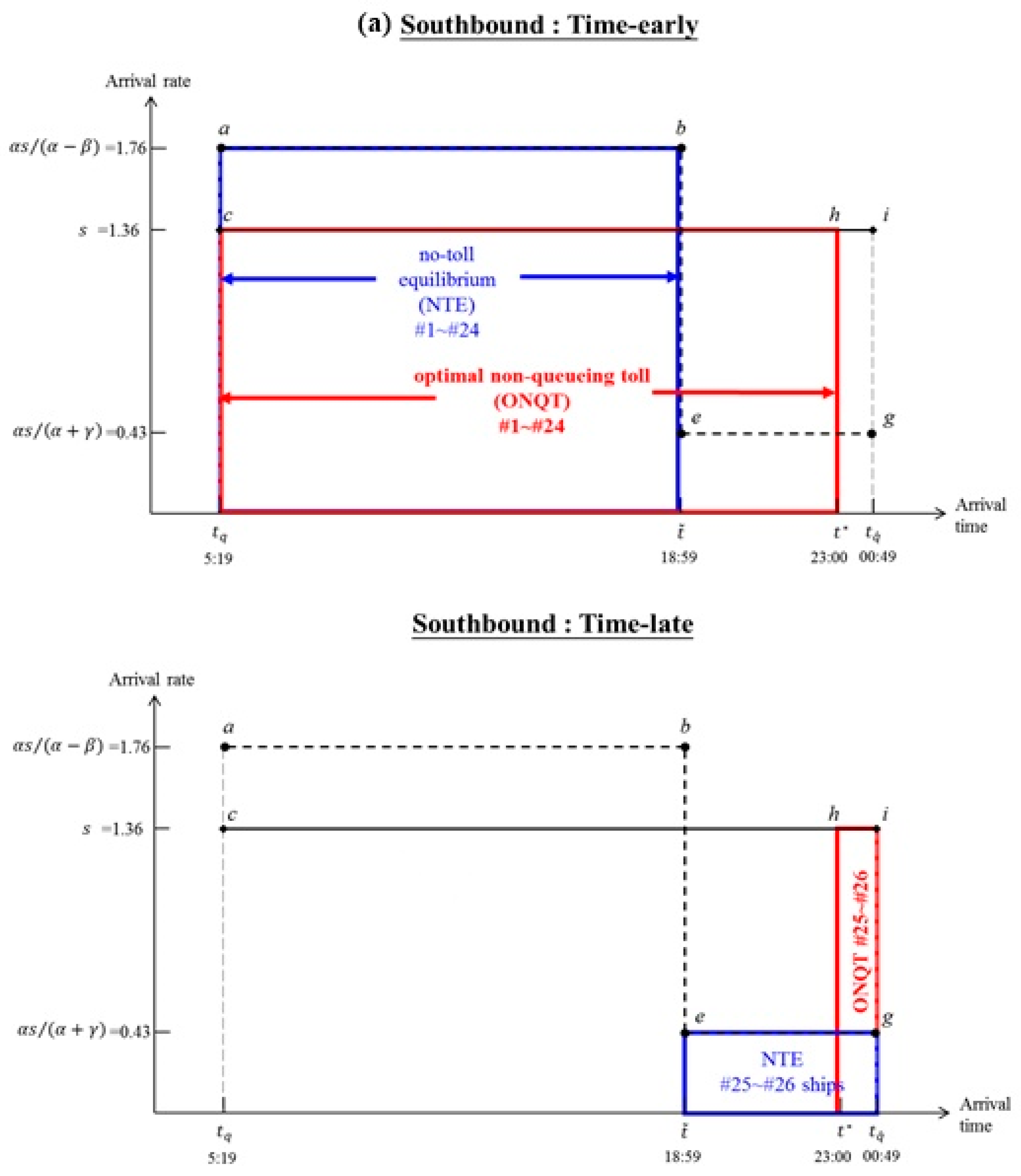
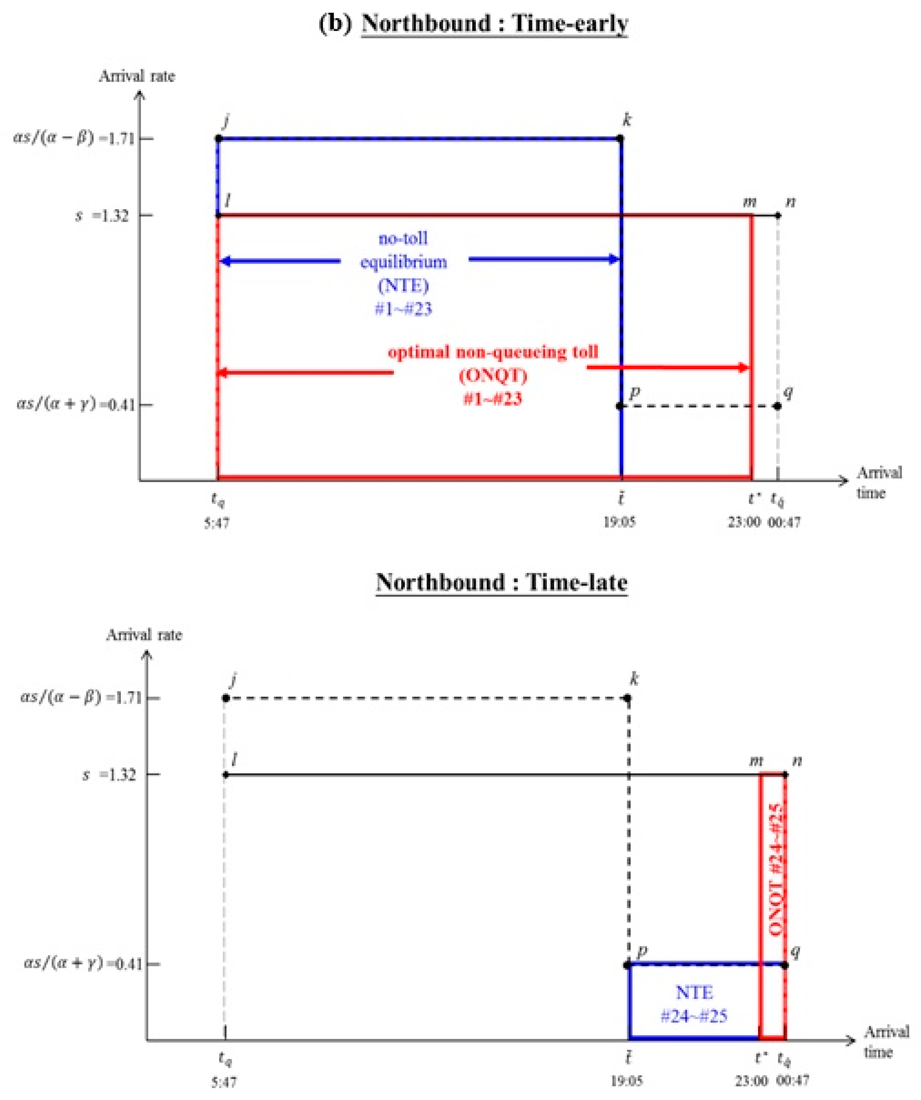
According to Table 4, Figure 2 indicates all ships’ arrival rates in the no-toll equilibrium, which are $\frac{\alpha \cdot S}{\alpha -\beta }=$ 1.76 and 1.71 for the early southbound (SB) and northbound (NB) ships, respectively, and $\frac{\alpha \cdot S}{\alpha +\gamma }=$ 0.43 and 0.41 for the delayed SB and NB ships, respectively. In the no-toll equilibrium, there are $\frac{\gamma \cdot N}{\beta +\gamma }=$ 24 and 23 early SB and NB ships, respectively, and the delayed ships is $\frac{\beta \cdot N}{\beta +\gamma }=$ 2 for both SB and NB ships. The horizontal lines ci and ln in Figure 2 represent the unique arrival rates, which are S = 1.36 and 1.32 for the SB, and NB ships, respectively, after the implementation of the optimal non-queueing toll scheme. In addition, time-early and time-late ships under this toll scheme are identical in number to those under the no-toll equilibrium.

In Figure 2, 24 early southbound ships must shift their original arrival time of 5:19~18:59 (5.32~18.99) in the no-toll case to 5:19~23:00 (5.32~23) in the tolled case. Ships #1 to #24 in rectangle $t_{q}ab\tilde{t}$ move to rectangle $t_{q}ch{t}^{*}$ in sequence because of the same time-early costs of $\beta \cdot T_E(t_q,\tilde{t})$ and $\beta \cdot T_E(t_q,t^{*})$ from the no-toll to the tolled case. Similarly, two delayed ships must shift their arrival times from 18:59~00:49 (18.99~24.82) in the no-toll case to 23:00~00:49 (23~24.82) in the tolled case to achieve equilibrium. That is, ships #25 and #26 in rectangle $\tilde{t}eg{t}_{q^{\prime }}$ move to rectangle $t^{*}hi{t}_{q^{\prime }}$ in sequence because of the same time-late costs of $\gamma \cdot T_L(\tilde{t},t_{q^{\prime }})$ and $\gamma \cdot T_L(t^{*},t_{q^{\prime }})$ from the no-toll to the tolled case.

In relation to the northbound ships in Figure 2, 23 early ships must shift their original arrival time of 5:47~19:05 (5.78~19.09) in the no-toll case to 5:47~23:00 (5.78~23) in the tolled case. Ships #1 to #23 in rectangle $t_{q}jk\tilde{t}$ move to rectangle $t_{q}lm{t}^{*}$ in sequence from the no-toll to the tolled case. Similarly, two delayed ships must shift their original arrival time of 19:05~00:47 (19.09~24.78) in the no-toll case to 23:00~00:47 (23~24.78) in the tolled case for equilibrium. That is, ships #24 and #25 in rectangle $\tilde{t}pq{t}_{q^{\prime }}$ move to rectangle $t^{*}mn{t}_{q^{\prime }}$ in sequence from the no-toll to the tolled case.

From the above results, all the tolled ships have clearly extended their previous arrival times and entered the New Suez Canal at the same times as they would in the no-toll equilibrium. Finally, such efficient ship movements caused by the levying of the optimal non-queueing tolls enable all ships to enter the canal without queueing.

For more details on each ship’s movement after tolling, we use Table 6 to show the numerical results according to timetable for 26 southbound ships from the no-toll to the tolled case in

Table 9. Numerical results according to timetable for southbound ships from the no-toll to the tolled case.

Southbound (SB)
No.	No-Toll Equilibrium			Optimal Non-Queueing Toll				Differences
	AT (t)	WT (h)	ET (t)	AT (t)	WT (h)	Toll (USD)	ET (t)	ΔAT(h)	ΔWT(h)	ΔET(h)
1	5.324	0.000	5.324	5.324	0.000	0.000	5.324	0.000	0.000	0.000
2	5.904	0.170	6.074	6.074	0.000	82.868	6.074	0.170	−0.170	0.000
3	6.484	0.340	6.824	6.824	0.000	165.735	6.824	0.340	−0.340	0.000
4	7.064	0.510	7.574	7.574	0.000	248.603	7.574	0.510	−0.510	0.000
5	7.644	0.680	8.324	8.324	0.000	331.470	8.324	0.680	−0.680	0.000
6	8.224	0.850	9.074	9.074	0.000	414.338	9.074	0.850	−0.850	0.000
7	8.804	1.020	9.824	9.824	0.000	497.205	9.824	1.020	−1.020	0.000
8	9.384	1.190	10.574	10.574	0.000	580.073	10.574	1.190	−1.190	0.000
9	9.964	1.361	11.324	11.324	0.000	662.940	11.324	1.361	−1.361	0.000
10	10.544	1.531	12.074	12.074	0.000	745.808	12.074	1.531	−1.531	0.000
11	11.124	1.701	12.824	12.824	0.000	828.675	12.824	1.701	−1.701	0.000
12	11.704	1.871	13.574	13.574	0.000	911.543	13.574	1.871	−1.871	0.000
13	12.283	2.041	14.324	14.324	0.000	994.410	14.324	2.041	−2.041	0.000
14	12.863	2.211	15.074	15.074	0.000	1077.278	15.074	2.211	−2.211	0.000
15	13.443	2.381	15.824	15.824	0.000	1160.145	15.824	2.381	−2.381	0.000
16	14.023	2.551	16.574	16.574	0.000	1243.013	16.574	2.551	−2.551	0.000
17	14.603	2.721	17.324	17.324	0.000	1325.880	17.324	2.721	−2.721	0.000
18	15.183	2.891	18.074	18.074	0.000	1408.748	18.074	2.891	−2.891	0.000
19	15.763	3.061	18.824	18.824	0.000	1491.615	18.824	3.061	−3.061	0.000
20	16.343	3.231	19.574	19.574	0.000	1574.483	19.574	3.231	−3.231	0.000
21	16.923	3.401	20.324	20.324	0.000	1657.350	20.324	3.401	−3.401	0.000
22	17.503	3.571	21.074	21.074	0.000	1740.218	21.074	3.571	−3.571	0.000
23	18.083	3.742	21.824	21.824	0.000	1823.085	21.824	3.742	−3.742	0.000
24	18.663	3.912	22.574	22.574	0.000	1905.953	22.574	3.912	−3.912	0.000
25	22.427	1.648	24.074	24.074	0.000	802.898	24.074	1.648	−1.648	0.000
26	24.824	0.000	24.824	24.824	0.000	0.000	24.824	0.000	0.000	0.000

. As 24 ships $\left(=\frac{\gamma \cdot N}{\beta +\gamma }\right)$ arrive at the anchorage of the New Suez Canal before the on-time arrival time $\tilde{t}=$ 18.99 = 18:59, ships #1 to #24 make up the time-early scheduling group, and ships #25 to #26 are the time-late scheduling group. For instance, ship #24, with the longest length of queuing time (3.91 h) in the no-toll equilibrium, has to be charged the highest toll (about USD1905.953) for zero queueing under the optimal non-queueing toll scheme. In addition, it could benefit from the longest arrival time extension (3.91 h) from 18:40 (AT = 18.66) in the no-toll case to 22:34 (AT = 22.57) in the tolled case.

In Table 9, both arrival time extension (ΔAT) and length of queuing time reduction (ΔWT) for the time-early scheduling from the no-toll to the tolled case show an increasing tendency from zero to 3.91 h (maximum) as the number of ships increases from 1 to 24. Thereafter, a decreasing trend toward zero for time-late scheduling is observed as the number of ships increases from 25 to 26. Furthermore, Table 9 shows that the amount of optimal non-queueing toll levied on a ship divided by the hourly queueing time cost ($\alpha$) corresponds to the ship’s arrival time extension (ΔAT) at the anchorage. For example, ΔAT (=3.91 h) for the ship #24 is identical to USD1905.953 divided by USD487.26.

Similarly, the numerical results according to timetable for the 25 northbound ships from the no-toll to the tolled case are shown in

Table 10. Numerical results according to timetable for northbound ships from the no-toll to the tolled case.

Northbound (NB)
No.	No-Toll Equilibrium			Optimal Non-Queueing Toll				Differences
	AT (t)	WT (h)	ET (t)	AT (t)	WT (h)	Toll (USD)	ET (t)	ΔAT(h)	ΔWT(h)	ΔET(h)
1	5.778	0.000	5.778	5.778	0.000	0.000	5.778	0.000	0.000	0.000
2	6.365	0.172	6.538	6.538	0.000	83.972	6.538	0.172	−0.172	0.000
3	6.953	0.345	7.298	7.298	0.000	167.945	7.298	0.345	−0.345	0.000
4	7.541	0.517	8.058	8.058	0.000	251.917	8.058	0.517	−0.517	0.000
5	8.128	0.689	8.818	8.818	0.000	335.890	8.818	0.689	−0.689	0.000
6	8.716	0.862	9.578	9.578	0.000	419.862	9.578	0.862	−0.862	0.000
7	9.304	1.034	10.338	10.338	0.000	503.834	10.338	1.034	−1.034	0.000
8	9.891	1.206	11.098	11.098	0.000	587.807	11.098	1.206	−1.206	0.000
9	10.479	1.379	11.858	11.858	0.000	671.779	11.858	1.379	−1.379	0.000
10	11.067	1.551	12.618	12.618	0.000	755.752	12.618	1.551	−1.551	0.000
11	11.654	1.723	13.378	13.378	0.000	839.724	13.378	1.723	−1.723	0.000
12	12.242	1.896	14.138	14.138	0.000	923.696	14.138	1.896	−1.896	0.000
13	12.830	2.068	14.898	14.898	0.000	1007.669	14.898	2.068	−2.068	0.000
14	13.417	2.240	15.658	15.658	0.000	1091.641	15.658	2.240	−2.240	0.000
15	14.005	2.413	16.418	16.418	0.000	1175.614	16.418	2.413	−2.413	0.000
16	14.593	2.585	17.178	17.178	0.000	1259.586	17.178	2.585	−2.585	0.000
17	15.180	2.757	17.938	17.938	0.000	1343.558	17.938	2.757	−2.757	0.000
18	15.768	2.930	18.698	18.698	0.000	1427.531	18.698	2.930	−2.930	0.000
19	16.355	3.102	19.458	19.458	0.000	1511.503	19.458	3.102	−3.102	0.000
20	16.943	3.274	20.218	20.218	0.000	1595.476	20.218	3.274	−3.274	0.000
21	17.531	3.447	20.978	20.978	0.000	1679.448	20.978	3.447	−3.447	0.000
22	18.118	3.619	21.738	21.738	0.000	1763.420	21.738	3.619	−3.619	0.000
23	18.706	3.791	22.498	22.498	0.000	1847.393	22.498	3.791	−3.791	0.000
24	22.348	1.670	24.018	24.018	0.000	813.603	24.018	1.670	−1.670	0.000
25	24.778	0.000	24.778	24.778	0.000	0.000	24.778	0.000	0.000	0.000

. Because 23 ships arrive at the anchorage before $\tilde{t}=$ 19.09 = 19:05, then ships #1 to #23 compose the time-early scheduling group, and ships of #24 and #25 make up the time-late scheduling group. For example, ship #23, with the longest length of queuing time (3.79 h) in the no-toll equilibrium, has to be charged the highest toll (USD1847.393) for zero queueing after tolling. This ship could benefit from the longest arrival time extension (3.79 h) from 18:43 (AT = 18.71) in the no-toll case to 22:30 (AT = 22.50) in the tolled case.

Similar to Table 9, it is clear from Table 10 that both arrival time extension (ΔAT) and length of queuing time reduction (ΔWT) show an increasing trend from 0 to 3.79 h (maximum) as the number of ships increases from 1 to 23. Thereafter, a decreasing tendency toward zero is seen as the number of ships increases from 24 to 25. Furthermore, taking ship #23 as an example, the toll (USD1847.39) levied on this ship divided by the hourly queueing time cost ($\alpha$ = USD487.26) is just equal to this ship’s arrival time extension (ΔAT = 3.79 h).

According to Table 9 and Table 10, the canal authority could implement an electronic canal pricing system with the timetable of arrival that each ship must comply with and the amount of optimal non-queueing toll that each ship should pay during the canal’s operating hours. Such an effective management could eliminate the phenomenon of ships waiting in line to enter the canal. For example, the captain of the 15th northbound ship in Table 10 would be informed by the canal authorities that the ship should pay USD1175.61 of the optimal non-queueing toll to enter the canal without queueing at 16:25 (AT = 16.42). From a shipowner’s perspective, this would be a pleasing toll scheme because he (she) could precisely control the sailing schedule to cross the canal without suffering a substantial loss of schedule delay due to queueing.

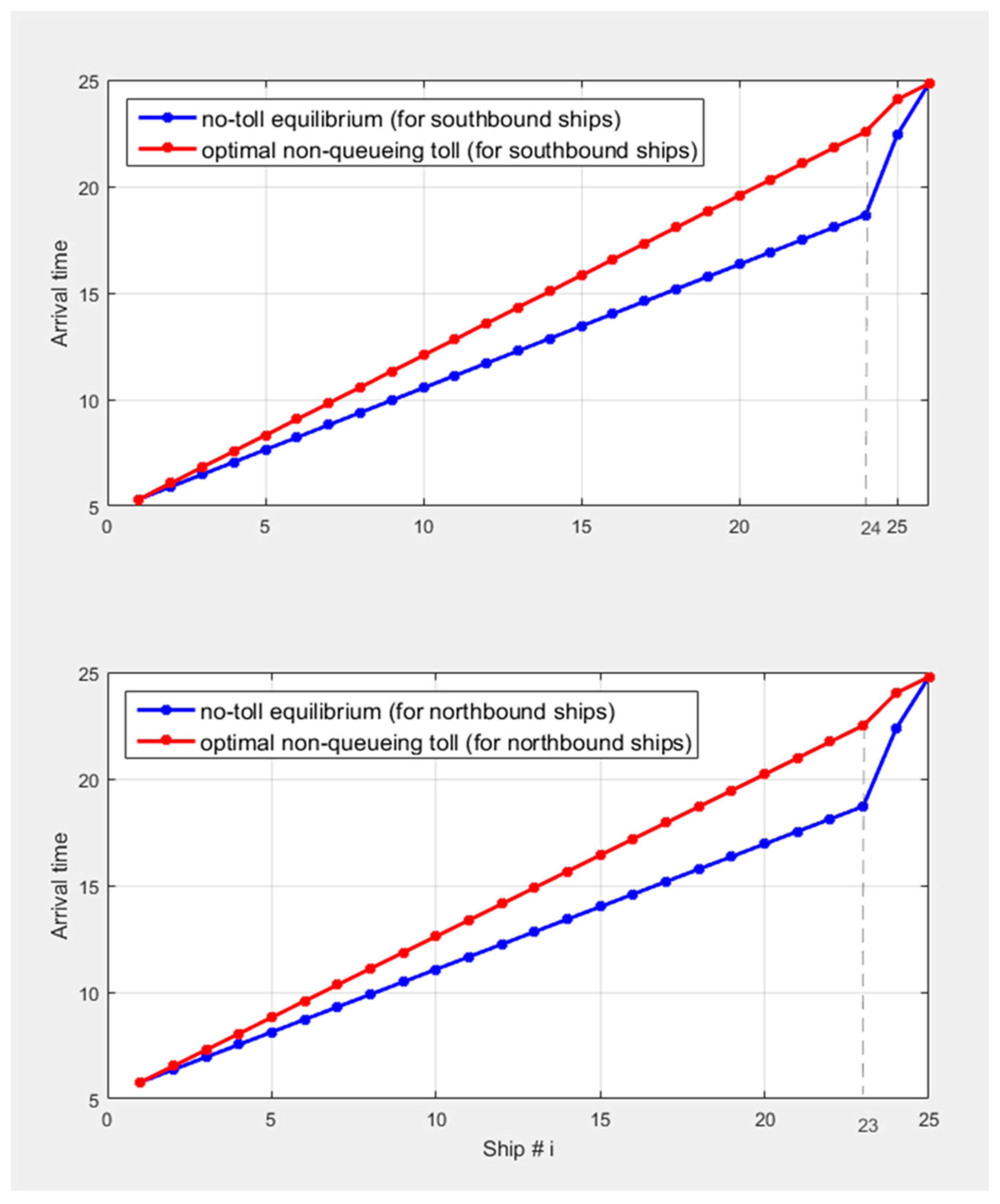
Figure 3 shows the relation between the individual ship and its corresponding arrival time for both the no-toll and tolled cases in this numerical example. The blue lines for the southbound and northbound ships are the original arrival time distributions in the no-toll equilibrium. In addition, the red lines for the southbound and northbound ships show the most efficient arrival time distribution to completely eliminate the total queueing time under the optimal non-queueing toll scheme. It is obvious from Figure 3 that all ships’ arrival times have been postponed from the no-toll blue line to the tolled red line. Moreover, since each ship’s arrival time on the red line is its canal entry time, the height between the red and blue lines will be the length of queueing time that could be saved for each ship to enter the canal if the optimal non-queueing toll scheme is implemented. It is clear that southbound ship #24 and northbound ship #23 correspond to the maximum vertical height in Figure 3. That is, the two ships will benefit from the largest arrival time extension after being charged with the highest toll.

5. Conclusions

The construction expansion of the New Suez Canal, completed in 2016, allowed more large ships passing through the canal to sail through Asia, Europe and Africa without making a detour around the Cape of Good Hope. In particular, in the current trend of large-sized ships in both the liner and tramp shipping markets, the expansion of the Suez Canal has brought in more ships than before. According to the Suez Canal Authority, the number of ships passing through the New Suez Canal annually has been rising since 2016, causing more ships to queue into the canal than before. As the queueing problem at the canal’s anchorage is anticipated to be more serious, an optimal non-queueing toll scheme, which involves continuous changes in the toll amount, has been established previously to solve the queueing problem. However, no information regarding all ships’ arrival time adjustments under the optimal non-queueing toll scheme is available from the previous literature for management decision and practical application. To solve this problem, we computed each ship’s arrival time interval in all circumstances before and after implementing the optimal non-queueing toll scheme. This helped us derive useful and simplified mathematical formulae to obtain the arrival time movement trajectory for each ship from the no-toll to the tolled case. In addition, all derived formulae of each ship’s arrival time at the anchorage and entry time into the canal are all counted from queueing start time to facilitate a mutual comparison.

All the tolled ships can benefit not only from reduced queueing time but also from extended arrival times from the no-toll to the tolled case. We have shown that the arrival time extensions for ships with time-early or time-late scheduling exhibit an increasing or decreasing tendency, respectively. Moreover, a crucial finding is that the amount of optimal non-queueing toll levied on a ship divided by the hourly queueing time cost corresponds to the ship’s arrival time extension at the anchorage from the no-toll to the tolled case. This finding helps us to forecast each ship’s arrival time adjustment once the optimal non-queueing toll scheme is implemented at the New Suez Canal.

According to our mathematical formulae, the canal authorities could implement an electronic canal pricing system with the timetable of arrival that each ship must comply with and the amount of optimal non-queueing toll that each ship should pay during the canal’s operating hours. Such an effective management could eliminate the phenomenon of ships waiting in line to enter the canal. From the shipowner’s perspective, this would be a pleasing toll scheme because the ship could just follow the timetable to enter the canal at the scheduled time without having to stop engines and queueing at the canal’s anchorage under the optimal non-queueing toll scheme. Avoiding stop-and-go in the anchorage zone with limited space would reduce the risk of ship manipulation, and the safety of the ship would be enhanced. Under the optimal non-queueing toll scheme, the captain could simply follow the canal authority’s instructions to enter the canal at the scheduled time without queueing. This would enable the captain precisely control the sailing schedule to cross the canal and lead to the significant reduction of fuel consumption of ships. Consequently, the shipowner’s operating profits could be substantially increased.

Finally, a numerical analysis based on the latest data and statistics for 2019 has provided the numerical results of each ship’s arrival time adjustment from the no-toll to the tolled case at the New Suez Canal. These results might be considerably conducive to the planning and implementation of the electronic toll collection system for the canal authorities. Meanwhile, these results would be instructive to both maritime economists and policymakers in evaluating the effects of the optimal non-queueing toll scheme on ships’ arrival time adjustments at the anchorage of the New Suez Canal. As the annual canal operation statistics and related data change, the results of the numerical analysis will also change. Therefore, annual updates of the statistics and data are necessary to maintain the arrivals timetable and the corresponding toll rates feasible and effective for the New Suez Canal.

References

- Laih, C.H.; Tsai, Y.C.; Chen, Z.B. Optimal non-queueing pricing for the Suez Canal. Marit. Econ. Logist. 2015, 17, 359–370. [Google Scholar] [CrossRef]
- Vickrey, W.S. Congestion theory and transport investment. Am. Econ. Rev. 1969, 59, 251–260. [Google Scholar]
- Small, K.A. The scheduling of consumer activities: Work trips. Am. Econ. Rev. 1982, 72, 467–479. [Google Scholar]
- Cohen, Y. Commuter welfare under peak-load congestion tolls: Who gains and who loses. Int. J. Transp. Econ. 1987, 14, 239–266. [Google Scholar]
- Braid, M. Uniform versus peak-load pricing of a bottleneck with elastic demand. J. Urban Econ. 1989, 26, 320–327. [Google Scholar] [CrossRef]
- Arnott, R.; De Palma, A.; Lindsey, R. Economics of a bottleneck. J. Urban Econ. 1990, 27, 111–130. [Google Scholar] [CrossRef]
- Laih, C.-H. Queueing at a bottleneck with single- and multi-step tolls. Transp. Res. Part A Policy Pract. 1994, 28, 197–208. [Google Scholar] [CrossRef]
- Laih, C.-H. Effects of the optimal step toll scheme on equilibrium commuter behaviour. Appl. Econ. 2004, 36, 59–81. [Google Scholar] [CrossRef]
- Small, K.A. The bottleneck model: An assessment and interpretation. Econ. Transp. 2015, 4, 110–117. [Google Scholar] [CrossRef] [Green Version]
- Laih, C.H.; Chen, K.Y. Economics on the optimal n-step toll scheme for a queueing port. Appl. Econ. 2008, 40, 209–228. [Google Scholar] [CrossRef]
- Laih, C.H.; Sun, P.Y. Effects of the optimal n-step toll scheme on bulk carriers queueing for multiple berths at a busy port. Transp. Policy 2013, 28, 42–50. [Google Scholar] [CrossRef]
- Sun, P.Y.; Laih, C.H.; Chen, C.L. Modeling the optimal pricing for nonscheduled trampers queueing for shared-use berths at a busy port. Int. J. Transp. Econ. 2016, 43, 361–378. [Google Scholar]
Figure 1.
Queueing time costs and optimal non-queueing tolls.
Figure 2.
(a) Numerical example of ships’ arrival time adjustments for the southbound ships from the no-toll to the tolled case. (b) Numerical example of ships’ arrival time adjustments for the northbound ships from the no-toll to the tolled case.
Figure 3.
Numerical results of arrival time adjustment for southbound (SB) and northbound (NB) ships from the no-toll to the tolled case.