Comparison between Model Test and Three CFD Studies for a Benchmark Container Ship


Department of Mechanical Engineering, Faculty of Engineering, ”Dunărea de Jos” University of Galati, 47 Domneasca Street, 800008 Galati, Romania
*
Author to whom correspondence should be addressed.
J. Mar. Sci. Eng. 2021, 9(1), 62; https://doi.org/10.3390/jmse9010062
Submission received: 25 November 2020
/
Revised: 21 December 2020
/
Accepted: 5 January 2021
/
Published: 8 January 2021
(This article belongs to the Special Issue Modeling of Ship Hydrodynamics)
Abstract
:An alternative to experiments is the use of numerical model tests, where the performances of ships can be evaluated entirely by computer simulations. In this paper, the free surface viscous flow around a bare hull model is simulated with three Computational Fluid Dynamics (CFD) software packages (FINE Marine, ANSYS CFD and SHIPFLOW) and compared to the results obtained during the experimental tests. The bare hull model studied is the Duisburg Test Case (DTC), developed at the Institute of Ship Technology, Ocean Engineering and Transport Systems (ISMT) for benchmarking and validation of the numerical methods. Hull geometry and model test results of resistance, conducted in the experimental facility at SVA Postdam, Nietzschmann, in 2010, are publicly available. A comparative analysis of the numerical approach and experimental results is performed, related to the numerical simulation of the free surface viscous flow around a typical container ship. Further, a comparative analysis between the results provided by NUMECA, ANSYS and SHIPFLOW is performed. Regarding the solution obtained, a satisfactory agreement between the towing test results and the computation results can be noticed. The minimum mean error was obtained through the SHIPFLOW case, 2.011%, which proved the best solution for the case studied.
1. Introduction
In recent decades, freight transport has become particularly important, being one of the most popular methods of transport. Container ships are being replaced by new, faster ships with a much larger capacity due to market demand. Therefore, the study and improvement of these ships are essential in order to achieve the required performance.
Ship resistance is a concept that is constantly being studied due to the changing environment of ship navigation and the tendency to improve ship performance, but also to improve the methods for resistance prediction. Testing the ships in towing tanks is the most accurate solution for the prediction of resistance, but it is costly and takes a long time. As technology has developed quite a lot and the computers have a much higher capacity, the determination of the characteristics of ships has been oriented towards numerical simulations [1].
Nowadays, Computational Fluid Dynamics (CFD) represents a standard design practice in solving the ship hydrodynamics problems worldwide [2,3]. Thus, various CFD studies investigated the added resistance and ship motion in various sea state conditions [4,5], in seakeeping [6] or to find the optimal hull form for resistance reduction and operational efficiency [7,8]. The speed performance of eight commercial ships including resistance and propulsion characteristics was evaluated using CFD results [9]. An increasing number of studies have brought attention to the influence of the roughness of a ship’s hull, and CFD modeling has also been used to predict the effects on ship resistance (see, for example, [10]), while an uncertainty analysis was performed using CFD simulations for four different ship models [11]. Novel CFD-based approaches were recently developed [12,13] to be used in conjunction with model test experiments. This has the potential to accurately predict the full-scale resistance of a marine surface ship.
The Duisburg Test Case (DTC) model is a well-known container ship, and its characteristics have been analyzed over the years in many research studies (such as [14,15,16,17]). In this paper, the novelty is that the model was simulated with three CFD programs and the simulation results were compared with the results of towing tests to determine the most appropriate program for the analysis of this type of vessel so that the results obtained will be as accurate as possible.
2. Case Study Ship
Several container ships have been developed over recent years: Duisburg Test Case (University of Duisburg Essen-2012), KRISO Container Ship (Korean Research Institute), JUMBO, MEGA JUMBO (SVA Postdam), Hamburg Test Case, etc. For this paper, the DTC (Duisburg Test Case) was investigated. A comparative analysis of the numerical approach and experimental results is performed in this study, related to the numerical simulation of the free surface viscous flow around a typical container ship. Further, a comparative analysis between the results obtained with three CFD software packages (NUMECA, ANSYS and SHIPFLOW) is performed.
3. Mathematical Model
The XCHAP solver (SHIPFLOW), the ISIS flow solver (NUMECA) and Fluent (ANSYS) are based on Navier–Stokes equations [19,20,21,22,23]. These equations describe the pressure, velocity and the density of the flow and they can be solved numerically.
The Navier–Stokes equations for an incompressible flow and the time continuity equation can be described as follows:
where: —time average velocity components in Cartesian directions, Cartesian coordinates, t—time, —volume force, p—time average pressure, —kinematic viscosity, dynamic viscosity, —density.
Solving the mass conservation equation and Newton’s second law known as the momentum conservation equation gives us the velocity and pressure field.
Mass conservation:
Momentum conservation:
where: D—fluid domain, —arbitrary control volume, —velocity, —volume force (normally gravity force), —constraints, = × , where σ is the constraint tensor, is the unit normal vector, —strain rate.
In general, flows around the hull of the ships are turbulent and a range of approximation models exists to describe the flow. In this paper, the k-ω SST model was used for the comparation between NUMECA, ANSYS and SHIPFLOW. Further, a comparison between the k-ω SST model (Shear-Stress Transport), k- BSL (base-line model) and EASM (Explicit Algebraic Stress Model) was provided for the SHIPFLOW case.
The first model used, k-ω SST, tries to give better results than the k-ε model and k-ω model [24], and in this case, the turbulent viscosity is related to the transport of turbulent sheer stress. The equations for this model are presented below, where F1 is the blending function:
For k:
For ω:
where: k—turbulent kinetic energy k = , —instantaneous velocity components in Cartesian directions, instantaneous pressure, —modeling coefficients for k- equations, —specific dissipation of turbulent kinetic energy, turbulent frequency, —the switching function for handling the change between the and equations.
The second model, k-ω BSL, is a blending model between k-ε and k-ω. The blending function and the cross-diffusion can be written as
where is cross-diffusion in the ω-equation.
The EASM model includes nonlinear terms [25]. The equation can be describes as
For stress tensor:
For turbulent viscosity:
where: —Kronecker’s delta, —turbulent dynamic viscosity, —strain rate, —rotation rate, —turbulent kinematic viscosity.
4. Numerical Approach
Systematic calculations were carried out using three CFD software packages: FINE Marine, ANSYS Fluent and SHIPFLOW.
FINE Marine is a CFD software dedicated to naval architecture and produced by NUMECA. Through three modules, complete numerical solutions can be generated: HEXPRESS (mesh generator), ISIS-CFD (flow solver) [19] and CFView (post-processing of the results). Moreover, the program includes the “Wizard” option that can guide you through setting up the configuration and making the mesh.
ANSYS Fluent is a software capable of performing thermo-fluid-dynamic simulations for industrial applications but can also be used in ship design. The Fluent module can be used separately or integrated in the ANSYS Workbench module [20], an interface that helps to obtain more efficient and flexible workflows where the user can change the geometry and create the mesh.
SHIPFLOW is a CFD software produced by Flowtech International AB, which focuses on numerical simulations and ship optimization. SHIPFLOW, similar to ANSYS, can be used independently or together with the SHIPFLOW CAESES [21,22] interface that allows an easy pre-processing of the hull’s characteristics, execution of solutions, post-processing and detailed management of the parameters, as well as their change.
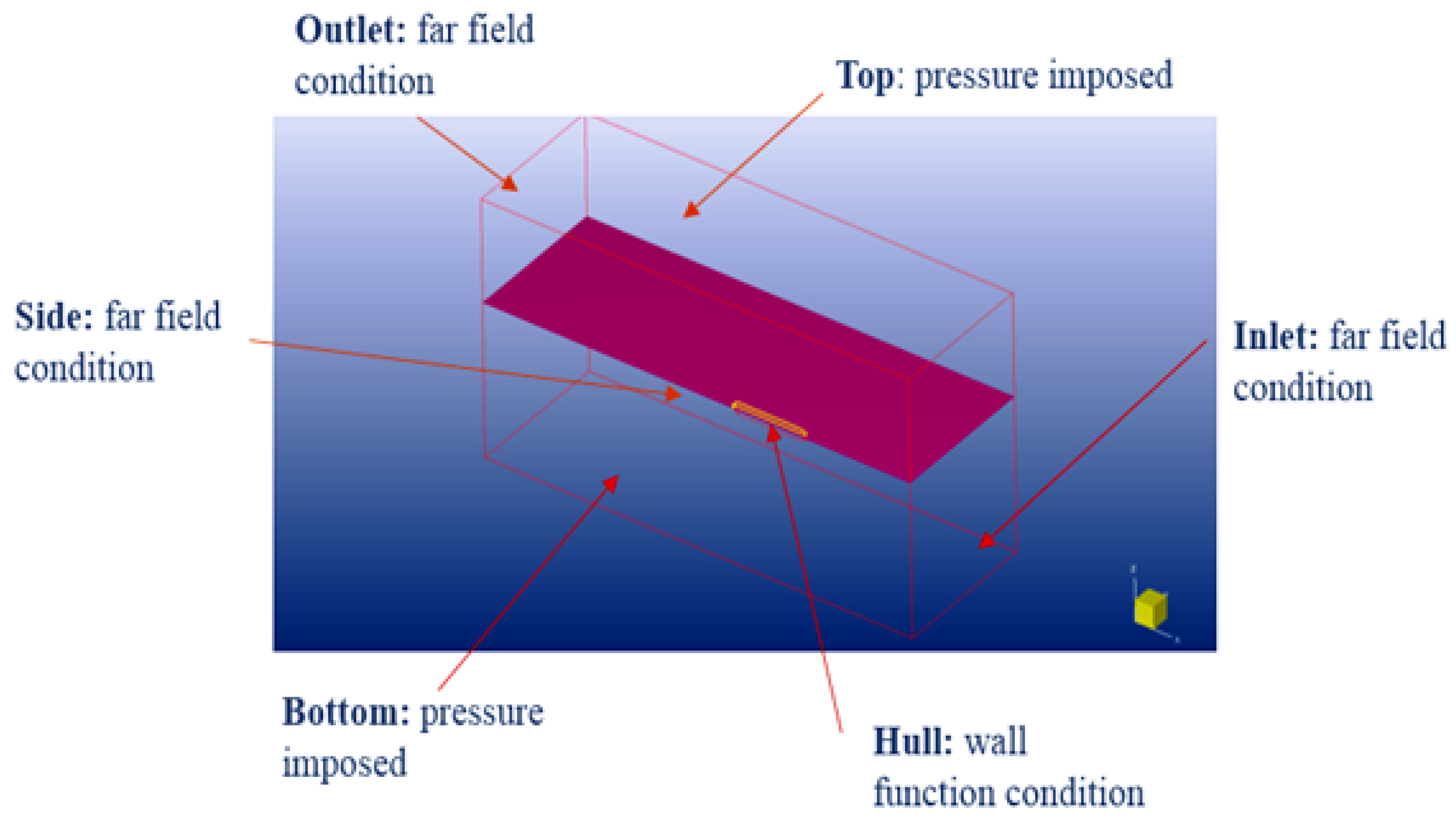
The same conditions were reproduced for all three programs. The domain is constructed by defining a box around the ship and is presented with the boundary conditions in Figure 2. The size of the computational domain is based on the length of the hull and extends [8,9] as follows: 1.5 length overall (Loa) in front of the ship’s hull, 3 Loa behind the hull, 1.5 Loa on the side, 1Loa above the ship’s hull and 1.5 Loa below the model’s keel.
The mesh was generated using a FINE/Marine plugin called C-Wizard [19] and HEXPRESS, the NUMECA grid generator [26,27]. The C-Wizard plugin is a helping tool that guides you through the whole process of setting the mesh and solver parameters.
Grid refinement is one of the most important steps when referring to fluid dynamics simulations [7,28,29], due to the major impact it has on the results obtained. A medium mesh was chosen with an extra refinement of the wave field. The effect of refinement around the free surface, based on wavelength, is to improve the accuracy of capturing the bow wave and the wave pattern behind the ship.
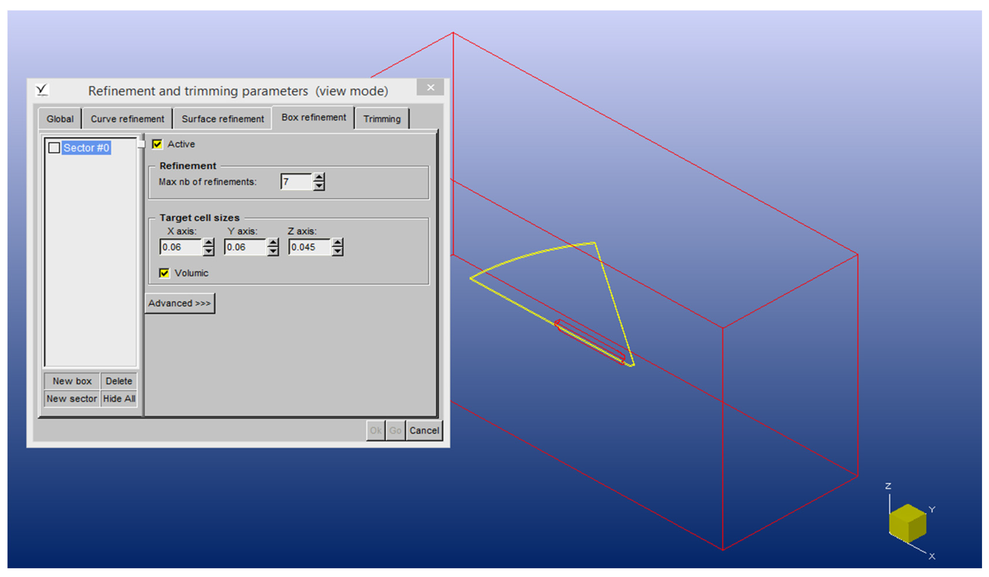
The mesh generation, using HEXPRESS, involves five steps: initial mesh, adapt to geometry, snap to geometry, optimize and viscous layers. The first step, initial mesh, is the module where the domain bounding box is subdivided along the Cartesian axis and an isotropic mesh is generated. In the second one, adapt to geometry, the cells go through several processes of refinement in different regions by splitting the initial volumes. For our case, a mix of refinement criteria was used (curve refinement for diametrical plan deck and transom; surface refinement for shaft, deck, transom and hull; box refinement for increasing the accuracy of the wave capturing (Figure 3)). In snap to geometry, the mesh is snapped onto the geometry and in the optimize step, the mesh is fixed for negative, concave or twisted cells and the quality of the mesh is increased. In the final step, to capture the viscous effect, a number of twelve layers was defined for shaft, transom, hull and deck, with a stretching ratio of 1.2.
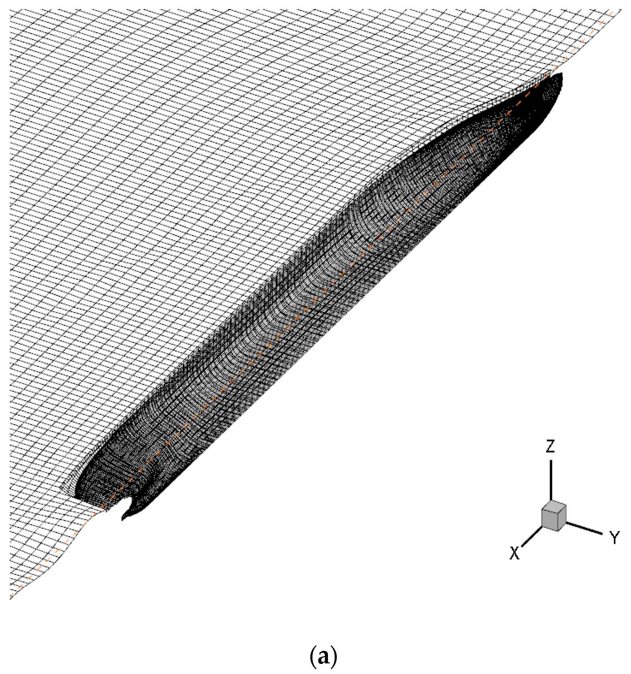
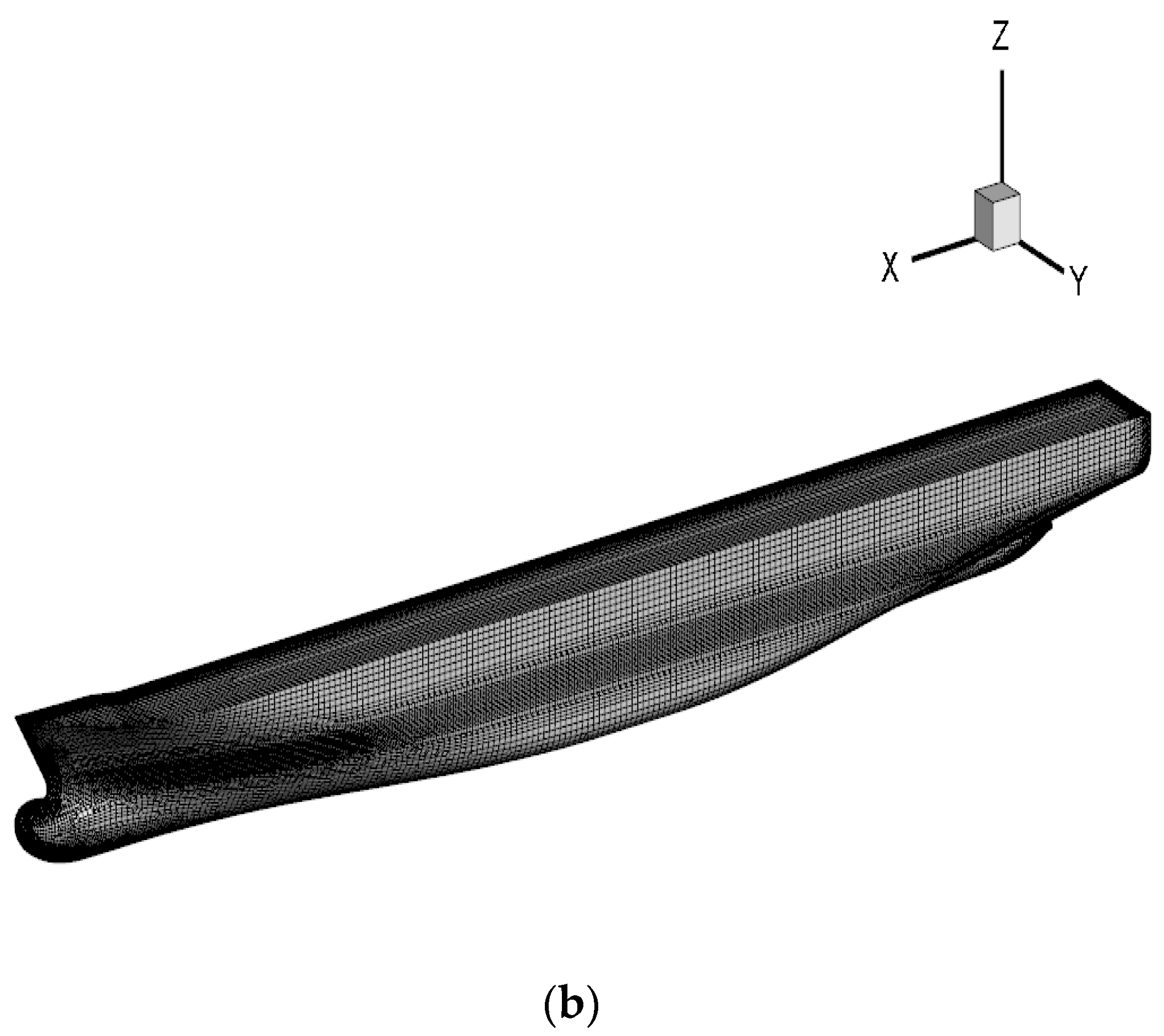
The grid generated in HEXPRESS was exported for use in ANSYS. One of the significant differences between the three CFD simulations is that, although the same network was used for the NUMECA and ANSYS simulations, for SHIPFLOW, the network was automatically generated a medium mesh by the program via the XMESH module. Another difference may be that the computer on which the network for NUMECA and ANSYS was generated, although it had special capabilities, was not as efficient as the one on which the network for SHIPFLOW was created, and therefore the network used for SHIPFLOW had a larger number of discretization cells (1,742,262 cells—SHIPFLOW, versus 1,481,236 cells—NUMECA/ANSYS; see Figure 4) but was performed using similar settings to the other mesh grid.
The setup for time configuration was chosen for a steady flow. The RANS flow solver [19,22,23] was used for all simulations using the Volume of Fluid (VOF) method (free surface capturing approach) and the k-ω (Menter Shear-Stress Transport [30]) turbulence model. The k-ω Shear-Stress Transport (SST) turbulence model, adopted to calculate the vortex viscosity, is a popular model used for performance in near-wall treatment and combines the k-ω turbulence model with the k- turbulence model. Further, this turbulence model is recommended for all basic hydrodynamic computations.
The theory of the VOF method and the turbulence model are explained in [3,19,20,21]. VOF is a numerical method used to model the boundaries of the free surface, in which the fixed network is designed for two or more immiscible fluids in which the position of the interface between fluids is part of the unknown found by the solution methodology.
The body motions, heave and trim, are solved using a quasi-static method, surge is imposed and sway, roll and yaw are fixed. The speed is defined in the center of gravity of the ship and, for each simulated speed, the ship starts from the initial speed of 0 m/second and the initial time of 0 s. The time step was set up to 0.02 s. The y+ parameter was set automatic, and the range of y+ varied from 0.12 to 1.5.
5. Numerical Simulation Results
Resistance was computed in calm water conditions and six speeds were studied: 1.335 m/s, 1.401 m/s, 1.469 m/s, 1.535 m/s, 1.602 m/s and 1.668 m/s. These speeds are correlated with the ship speeds used in towing tanks experiments. The results were processed and analyzed using Tecplot (a data visualization and CFD post-processing software [31]).
The computation was performed on parallel computers with four processors for the NUMECA case and 10 processors for the ANSYS and SHIPFLOW cases. The real simulation times for the solution to reach convergence were about 30 min for SHIPFLOW, around 2 h for ANSYS and 24 h, reaching even 48 h, for NUMECA. The fact that the computations in SHIPFLOW and ANSYS were made on parallel computers with more processors than the one the NUMECA simulations were conducted on led to this considerable difference in real time.
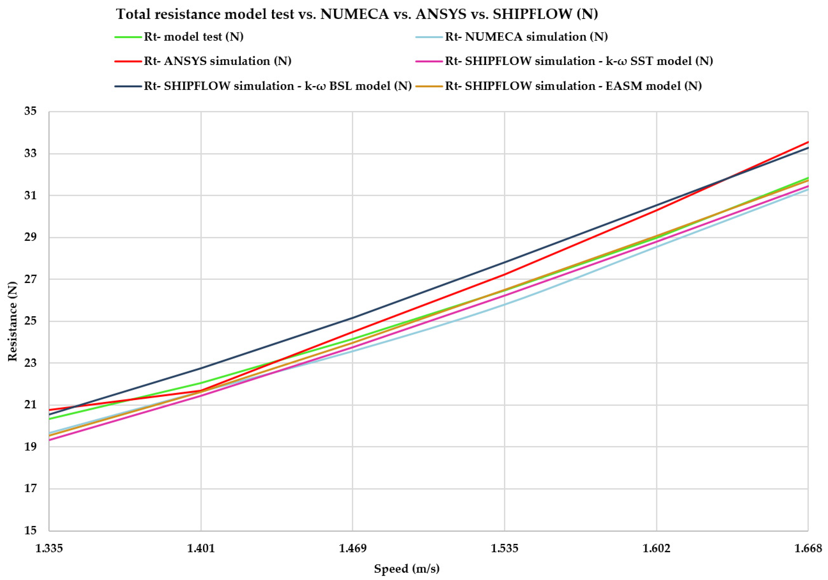
Upon completion of the numerical simulations using NUMECA, ANSYS and SHIPFLOW, the total resistance was generated for all speeds. The results of the three simulations were compared with the total resistance values available from model tests. For each speed, the discrepancy between the test and simulation results was established through the percentage error (PE), which is given by the following relationship:
As can be seen in Table 2 and Figure 5, a satisfactory agreement exists between the test and simulation results. SHIPFLOW generated better solutions than ANSYS Fluent and NUMECA, comparative to the model test regarding the simulation of the free surface around the Duisburg Test Case hull. All simulation results were close to the values of the towing test results. The solution obtained using SHIPFLOW has a lower error (see Table 2) compared with NUMECA and ANSYS solutions. Comparative to SHIPFLOW analysis, where the medium percentage error over the speed domain between the model test and numerical simulation is about 2.01%, for the NUMECA case, the medium percentage error is 2.16 and for the ANSYS case 2.98%.
In order to observe the influence of turbulence, in SHIPFLOW, for the same speed range, two more turbulence models were simulated besides k-ω SST, k-ω BSL and EASM. In the case of turbulence models, the closest results to the test model were achieved by the EASM model with a difference over the speed domain of 1.23%, compared to 2.01% in the case of k-ω SST and 3.9% in the case of k-ω BSL.
As the speed increases, the resistance increases, due to the increase in its components: frictional resistance and wave resistance. Therefore, the most conclusive difference for the three cases can be observed at the highest speed, 1668 m/s, where the percentage error is 1.19% for SHIPFLOW, 1.7% for NUMECA and 5.44% for ANSYS. It can be seen that although in NUMECA and SHIPFLOW simulations, with the increase in the speed, the solution stabilizes faster and the percentage error is smaller, instead for ANSYS at the speed of 1.668 m/s, the highest percentage error resulted.
Since ANSYS is a software used lately in the naval industry when the resistance of a ship or how it behaves in waves is required to be simulated, many users turn to use SHIPFLOW or NUMECA, these being known as software dedicated to numerical simulations in the naval field. On the other hand, for studying the free surface viscous flow around a ship, using ANSYS seems to be more difficult to reproduce the conditions necessary, but with a good knowledge of the software, the initial difficulties can be overcome. Through this study, we also tried to present some options that we have when we want to perform CFD simulations for ships.
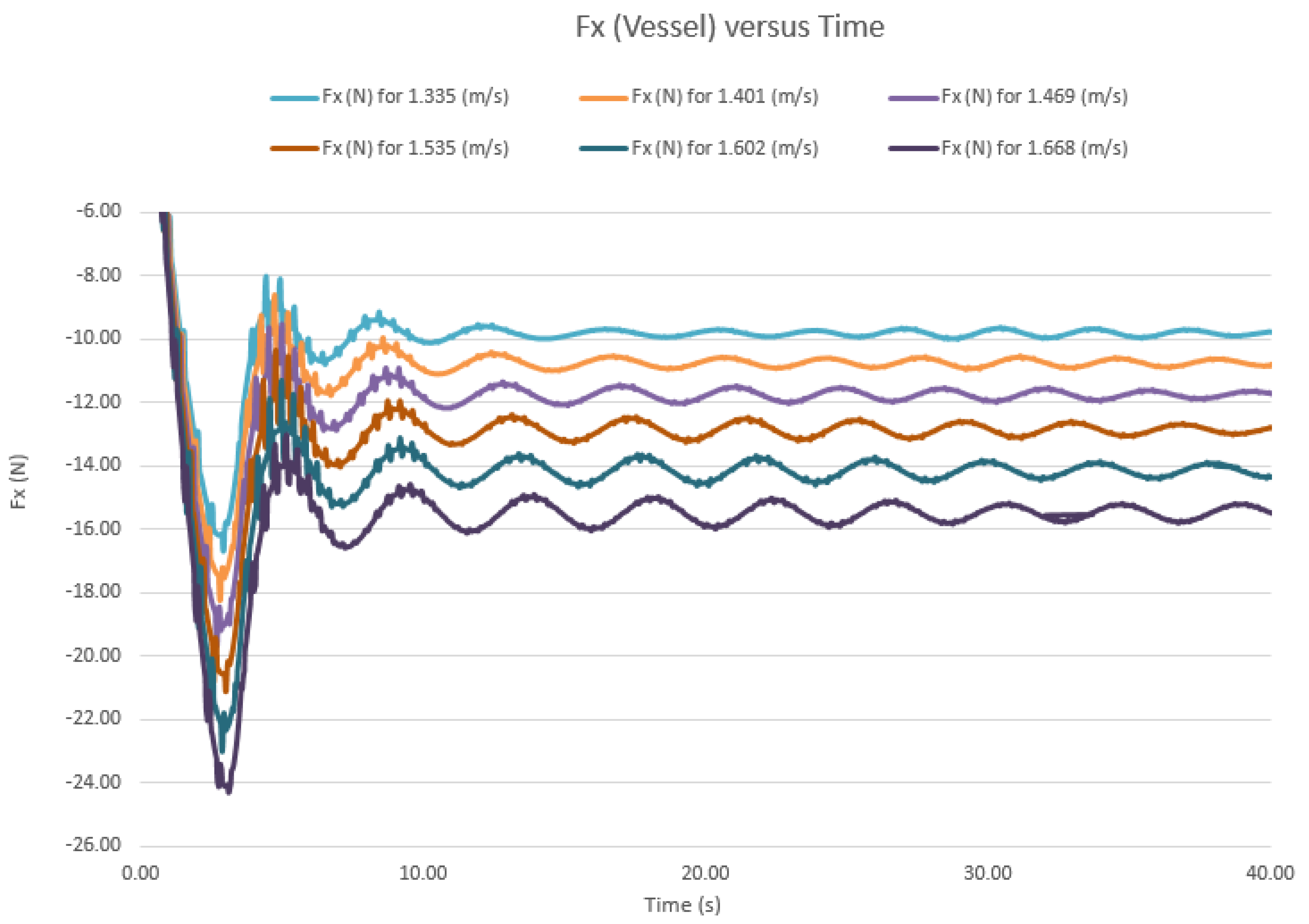
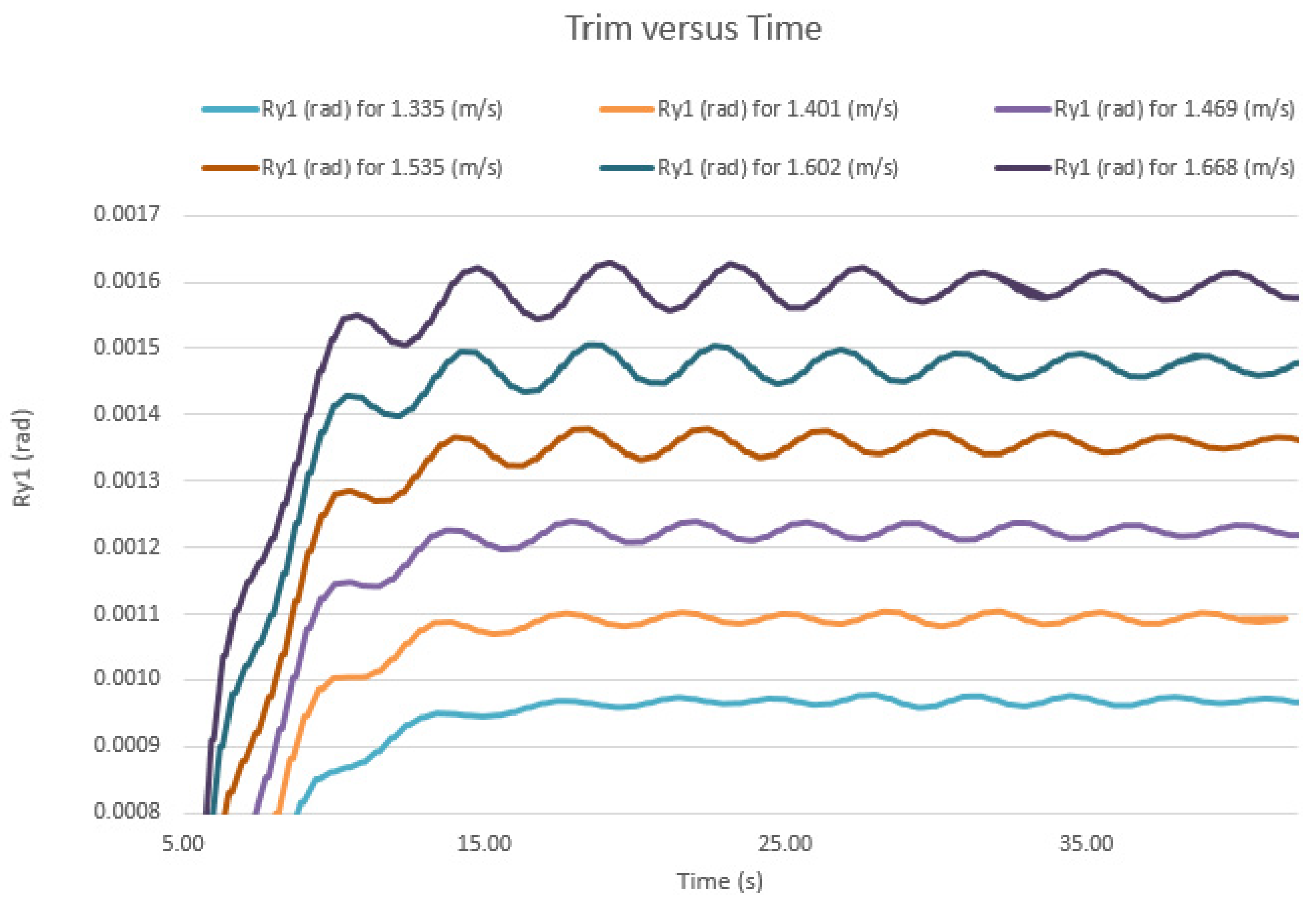
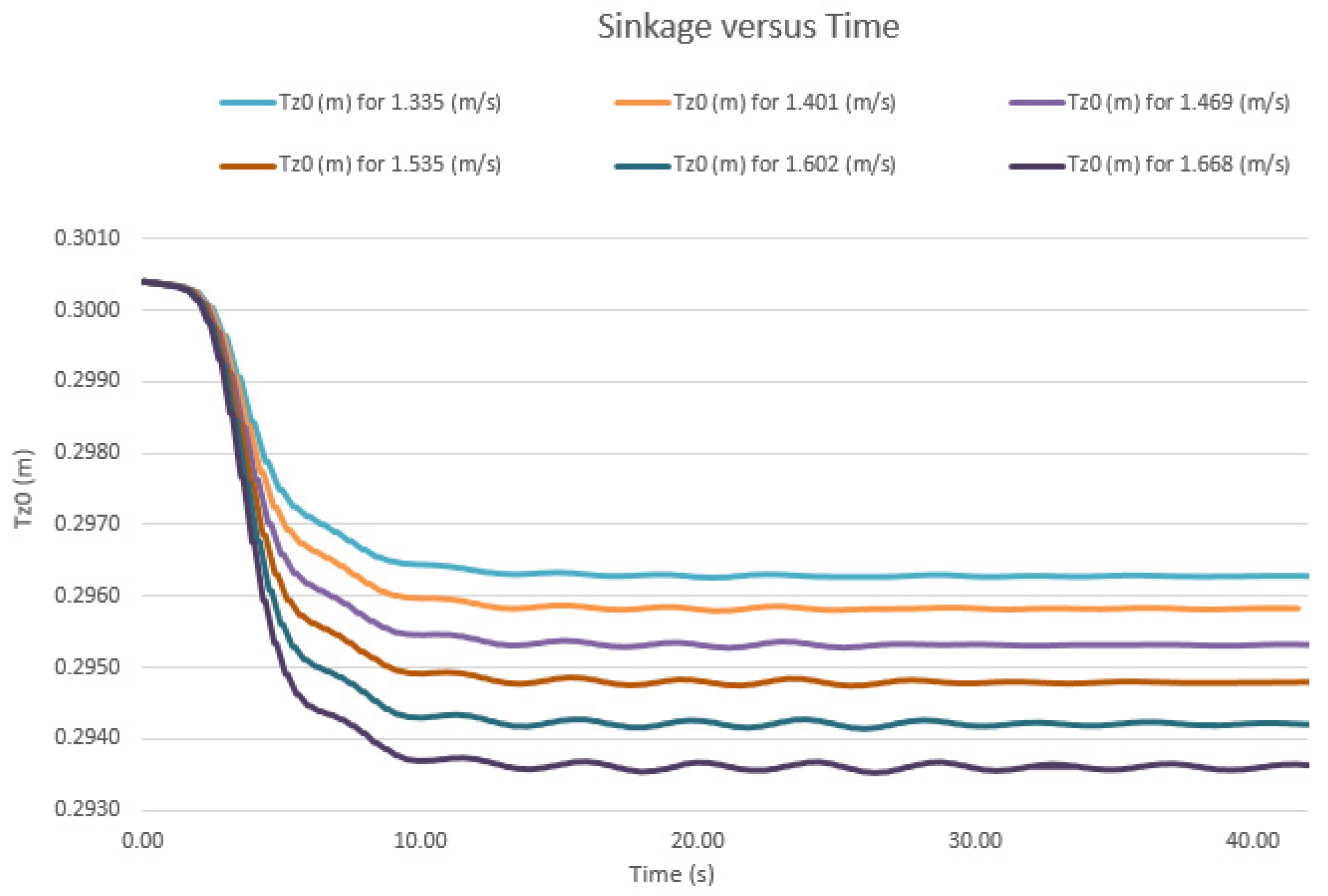
Since the simulation results in SHIPFLOW are the most optimal, the obtained results were processed in Tecplot for a better visualization and analysis of the obtained solution. The three main factors that are important when studying a ship are: sinkage, trim and resistance. The following figures (Figure 6, Figure 7 and Figure 8) show the results for the force on the X-axis (Fx (N)), trim (Ry1 (rad)) and sinkage (Tz0 (m)). The trim is the translation of the center of gravity of the body along the Z-axis in the initial position of reference.
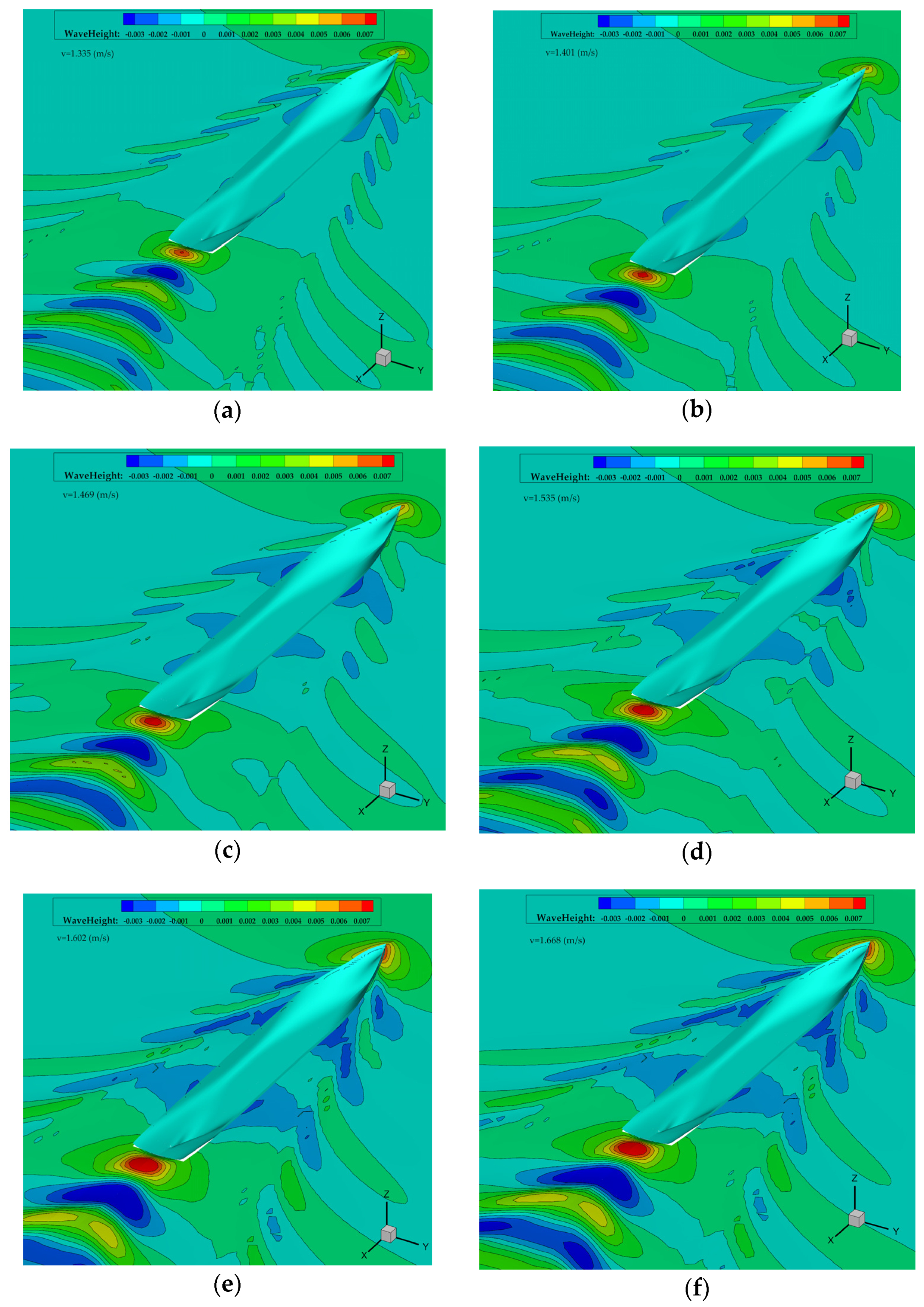
In Figure 9, the wave height generated for all six speeds in SHIPFLOW and processed in Tecplot is presented. As the speed increases, it can be seen that as the wave height increases, the wave component is also more visible.
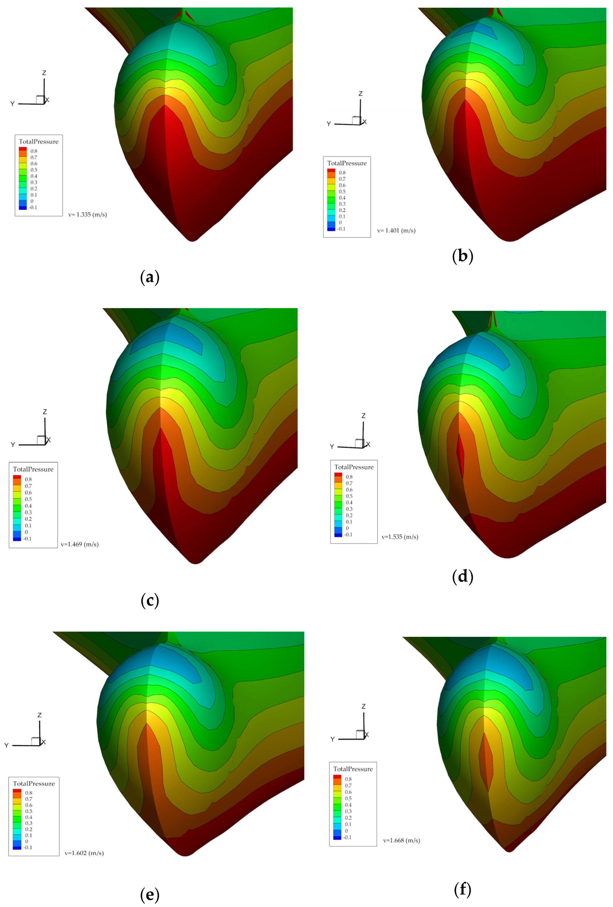
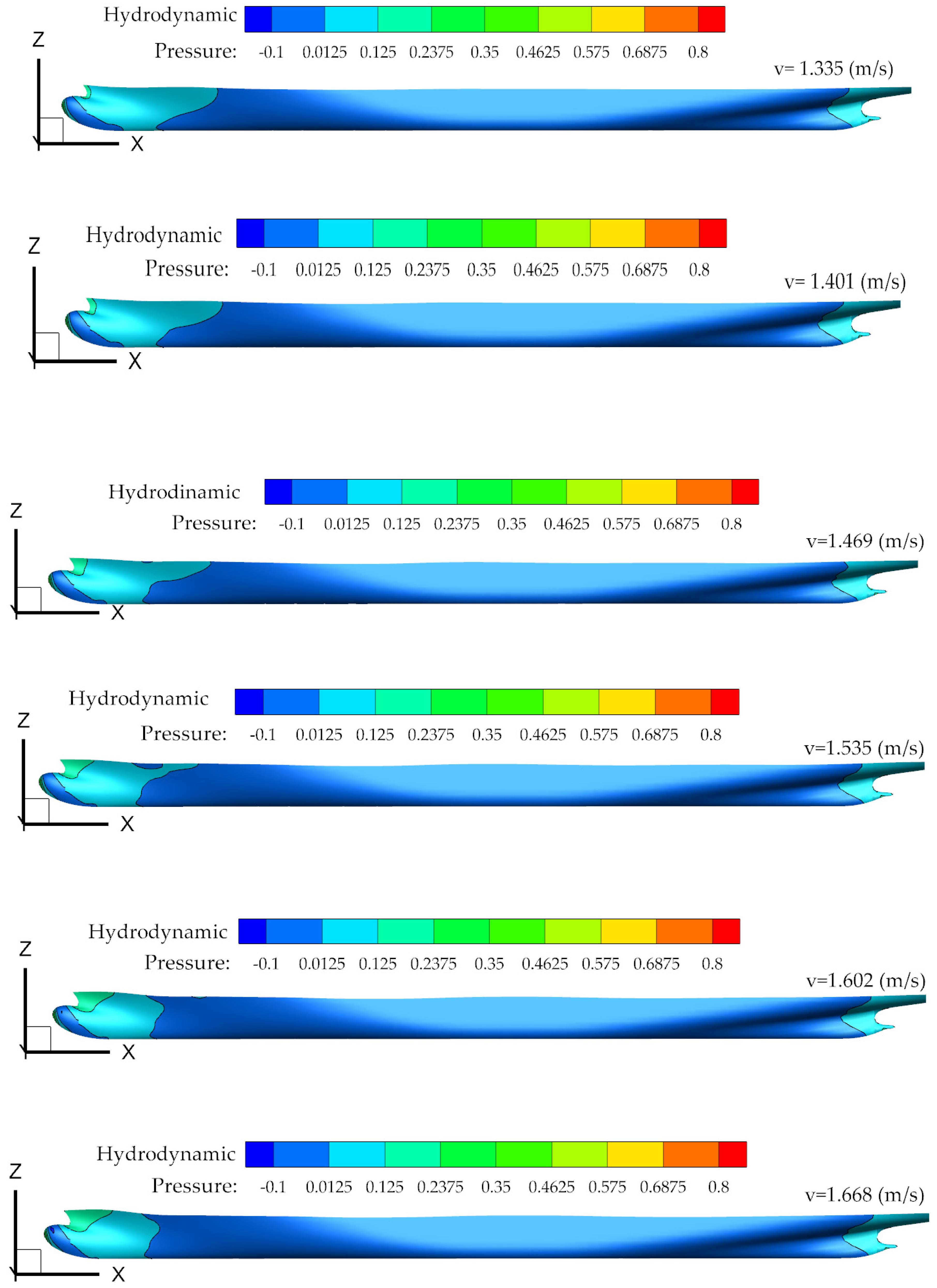
In Figure 10, the total pressure is presented, and in Figure 11, the hydrodynamic pressure is presented, both processed in Tecplot for all numerical simulations. The pressure variation around the ship’s bulb is normal for this type of ship. The pressure around the ship is calculated through all the computational volume, from the inlet to the outlet. The total pressure contains both the influence of the static pressure and of the hydrodynamic pressure. Further, we can see that for steady flows, the initial acceleration waves cause time-dependent values which are explained in Reference [32].
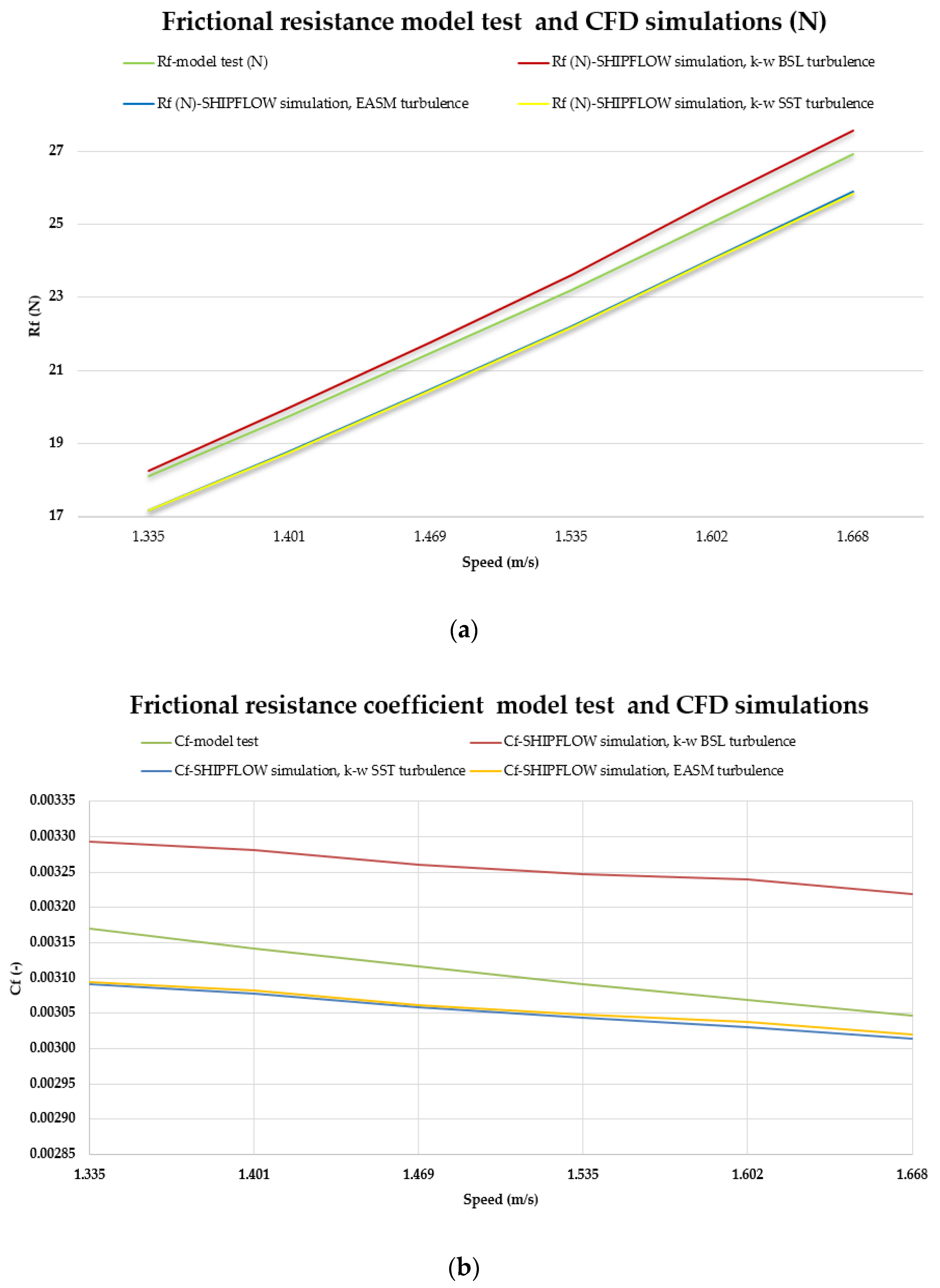
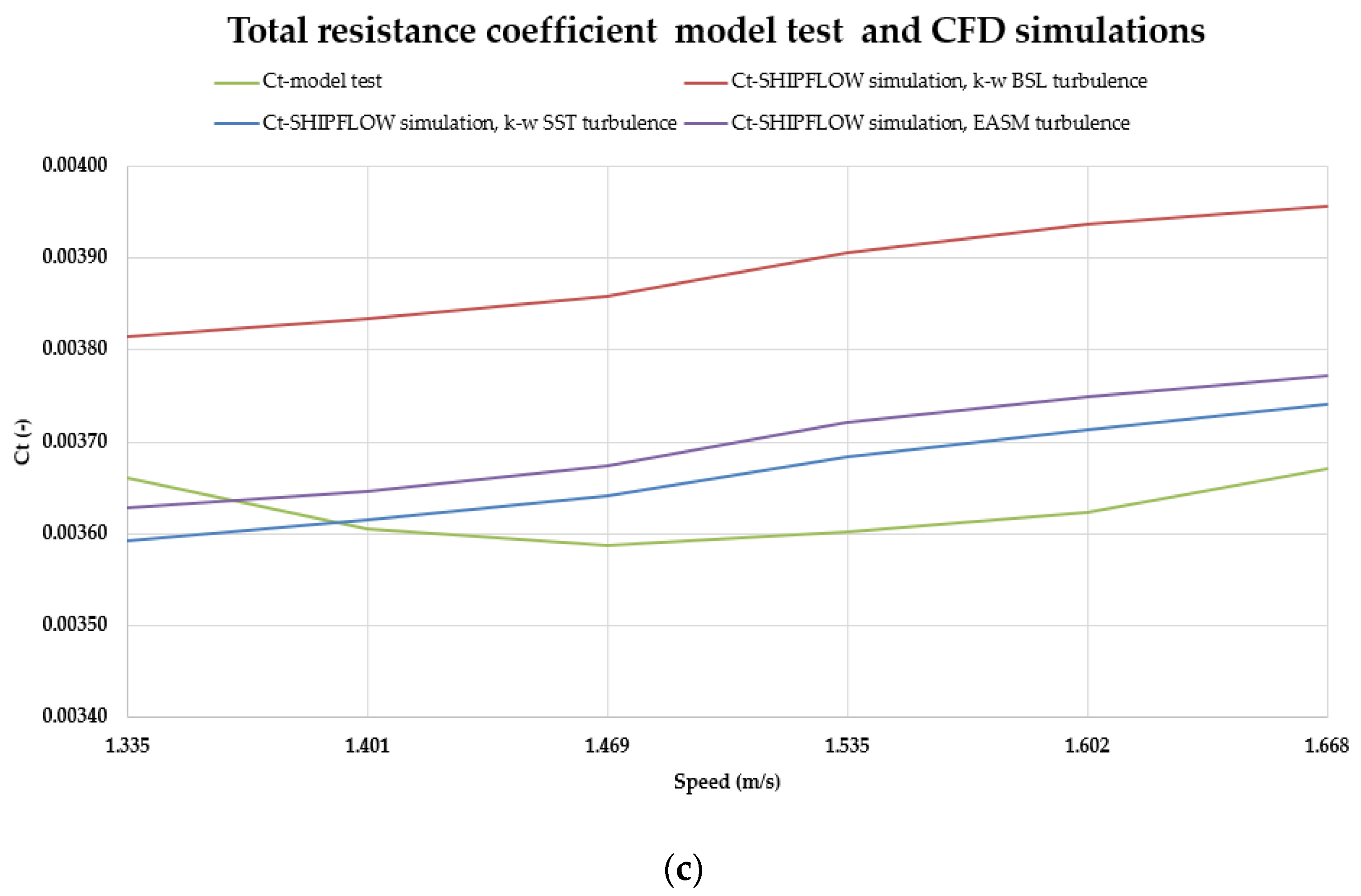
In Figure 12a, a comparison between the frictional resistance values from the CFD simulations and experimental tests is presented, while in Table 3, the percentage errors (computed following Equation (1)) between experimental tests and CFD simulations for the non-dimensional frictional resistance coefficient Cf (calculated according to ITTC 57), non-dimensional total resistance coefficient Ct and frictional resistance Rf (N) are presented. From Figure 12 and the PE values presented in Table 3, Table 4 and Table 5, a good agreement between the model tests and CFD simulations for all parameters can be observed.
6. Conclusions
Due to population growth and economic development, maritime transport has increased, and faster and safer transport solutions have led to find container ships with an optimized design according to these requirements. The current trend is to replace existing ships with new ones, which can carry a much larger cargo and can reach their destination faster. Therefore, this type of ship must be investigated and tested in order to optimize and improve ships.
Systematic calculations were carried out, for six different speeds, aiming to determine the characteristics of ship resistance. The hull studied was the Duisburg Test Case, a benchmark container ship used for validation of numerical methods and the results of the towing test are publicly available.
Three numerical simulations were carried out in order to determine the accuracy of the NUMECA, SHIPFLOW and ANSYS software packages in relation to the model test. The results are presented in this study and they show that more accurate solutions were obtained using SHIPFLOW, instead of using NUMECA or ANSYS simulations, leading to a medium percentage error of 2.01%. The results of numerical simulations can be improved by increasing the time steps and by changing the precision of the mesh, which would increase the accuracy of the results of the total resistance.
One of the reasons why the simulation results in SHIPFLOW had the lowest range of errors is that the grid used had a larger number of cells, which is allowed due to the superior capabilities of the computer on which the simulation was performed. Another reason why these differences between computations appeared, although the methodology was largely the same for all three software packages, is the use of default values for some parameters, such as relaxing factors. Further, the differences in results between the model and CFD simulations arise from the idealization of mathematical equations, as well as their limitations. The conditions imposed by the software solutions used to achieve convergence also play an important role in the development of these differences. As future work, a sensitivity study will be performed in which the extent to which some parameters can affect the accuracy of the results will be assessed.
In conclusion, Computational Fluid Dynamics (CFD) techniques are improving and now are frequently used to augment, and occasionally replace, the experiments. When we talk about CFD, we have a few advantages but also disadvantages compared to model tests. Speed, easy way to change the configuration and parameters and lower price are the main advantages, but the level of accuracy remains the main problem.
Author Contributions
Conceptualization, A.-M.C. and L.R.; software simulations, validation, analysis and visualization, A.-M.C.; writing—original draft preparation, A.-M.C.; supervision and writing final version, L.R. All authors have read and agreed to the published version of the manuscript.
Funding
This research received no external funding.
Institutional Review Board Statement
Not applicable.
Informed Consent Statement
Not applicable.
Data Availability Statement
The data presented in this study are openly available in https://www.uni-due.de/imperia/md/content/ist/dtc_str_vol50no3.pdf, reference number [18].
Conflicts of Interest
The authors declare no conflict of interest.
References
- Molland, A.F.; Turnock, S.R.; Hudson, D.A. Ship Resistance and Propulsion; Cambridge University Press: Cambridge, UK, 2017. [Google Scholar]
- Campana, E.F.; Peri, D.; Tahara, Y.; Stern, F. Shape optimization in ship hydrodynamics using computational fluid dynamics. Comput. Methods Appl. Mech. Eng. 2006, 196, 634–651. [Google Scholar] [CrossRef]
- Zhang, Z.R.; Hui, L.; Zhu, S.P.; Feng, Z.H.A.O. Application of CFD in ship engineering design practice and ship hydrodynamics. J. Hydrodyn. Ser. B 2006, 18, 315–322. [Google Scholar] [CrossRef]
- Liu, C.; Chen, G.; Wan, D. CFD Study of Added Resistance and Motion of DTC in Short and Long Waves. In Proceedings of the International Conference on Offshore Mechanics and Arctic Engineering (OMAE 2018), Madrid, Spain, 17–22 June 2018; American Society of Mechanical Engineers: New York, NY, USA, 2018; Volume 51265, p. V07AT06A011. [Google Scholar]
- Tezdogan, T.; Demirel, Y.K.; Kellett, P.; Khorasanchi, M.; Incecik, A.; Turan, O. Full-scale unsteady RANS CFD simulations of ship behaviour and performance in head seas due to slow steaming. Ocean Eng. 2015, 97, 186–206. [Google Scholar] [CrossRef] [Green Version]
- D’Aure, B.; Mallol, B.; Hirsch, C. (NUMECA Int. Belgium) Resistance and Seakeeping CFD Simulations for the KOREAN Container Ship. In Proceedings of the Tokyo Workshop, Tokyo, Japan, 2–4 December 2015. [Google Scholar]
- Diez, M.; Campana, E.F.; Stern, F. Stochastic optimization methods for ship resistance and operational efficiency via CFD. Struct. Multidiscip. Optim. 2018, 57, 735–758. [Google Scholar] [CrossRef]
- Liu, Z.; Liu, W.; Chen, Q.; Luo, F.; Zhai, S. Resistance reduction technology research of high-speed ships based on a new type of bow appendage. Ocean Eng. 2020, 206, 107246. [Google Scholar] [CrossRef]
- Choi, J.E.; Min, K.S.; Kim, J.H.; Lee, S.B.; Seo, H.W. Resistance and propulsion characteristics of various commercial ships based on CFD results. Ocean Eng. 2010, 37, 549–566. [Google Scholar] [CrossRef]
- Song, S.; Demirel, Y.K.; Atlar, M.; Dai, S.; Day, S.; Turan, O. Validation of the CFD approach for modelling roughness effect on ship resistance. Ocean Eng. 2020, 200, 107029. [Google Scholar] [CrossRef] [Green Version]
- Islam, H.; Soares, C.G. Uncertainty analysis in ship resistance prediction using OpenFOAM. Ocean Eng. 2019, 191, 105805. [Google Scholar] [CrossRef]
- Haase, M.; Zurcher, K.; Davidson, G.; Binns, J.R.; Thomas, G.; Bose, N. Novel CFD-based full-scale resistance prediction for large medium-speed catamarans. Ocean Eng. 2016, 111, 198–208. [Google Scholar] [CrossRef] [Green Version]
- Niklas, K.; Pruszko, H. Full-scale CFD simulations for the determination of ship resistance as a rational, alternative method to towing tank experiments. Ocean Eng. 2019, 190, 106435. [Google Scholar] [CrossRef]
- El Moctar, O.; Sigmund, S.; Schellin, T.E. Numerical and Experimental Analysis of Added Resistance of Ships in Waves. In Proceedings of the ASME 2014 34th International Conference on Ocean, Offshore and Arctic Engineering, OMAE2015-42403, St. John’s, NL, Canada, 31 May–5 June 2015. [Google Scholar]
- Ley, J.; Sigmund, S.; el Moctar, O. Numerical Prediction of the Added Resistance of Ships in Waves. In Proceedings of the 33rd International Conference on Ocean, Offshore, and Arctic Engineering, San Francisco, OMAE, San Francisco, CA, USA, 8–13 June 2014; Volume 24216, p. 2014. [Google Scholar]
- Riesner, M.; el Moctar, O. A time domain boundary element method for wave added resistance of ships taking into account viscous effects. Ocean Eng. 2018, 162, 290–303. [Google Scholar] [CrossRef]
- Xia, L.; Yuan, S.; Zou, Z.; Zou, Z. Uncertainty quantification of hydrodynamic forces on the DTC model in shallow water waves using CFD and non-intrusive polynomial chaos method. Ocean Eng. 2020, 198, 106920. [Google Scholar] [CrossRef]
- El Moctar, O.; Shigunov, V.; Zorn, T. Duisburg Test Case: Post-panamax container ship for benchmarking. Ship Technol. Res. Schiffstechnik 2012, 59, 50–64. [Google Scholar] [CrossRef]
- Theoretical Manual ISIS-CFD. NUMECA Fine/Marine; Version 6.2; NUMECA International: Brussels, Belgium, 2017. [Google Scholar]
- Tutorial Ship Hull—Free Surface Flow around a Ship Hull Using ANSYS Fluent; ANSYS: Canonsburg, PA, USA, 2016.
- SHIPFLOW 6.4 User’s Manual, Flowtech International AB, Rev. 6.4, Gothenburg, Sweden. Available online: http://www.flowtech.se (accessed on 27 February 2020).
- XCHAP. Theoretical Manual, 2007.
- Ansys Fluent. Theory Guide, ANSYS, Inc. Release 15.0, Southpointe, November 2013, 275 Technology Drive Canonsburg, PA 15317 ANSYS, Inc. is Certified to ISO 9001:2008. Available online: http://www.ansys.com (accessed on 27 February 2020).
- Menter, F.R. Zonal Two Equation k-ω Turbulence Models for Aerodynamic Flows. In Proceedings of the 24th Fluid Dynamics Conference, Orlando, FL, USA, 6–9 July 1993. [Google Scholar]
- Deng, G.B.; Queutey, P.; Visonneau, M. Three-Dimensional Flow Computation with Reynolds Stress and Algebraic Stress Models; Elsevier: Amsterdam, The Netherlands, 2005. [Google Scholar]
- Chirosca, A.M. Numerical Simulation of the Free Surface Viscous Flow around a Bare Hull Model. Master’s Thesis, Faculty of Naval Architecture, “Dunarea de Jos” University of Galati, Galați, Romania, 2019. [Google Scholar]
- Chirosca, A.M.; Gasparotti, C. Comparison between Model Test and Numerical Simulations for a Container ship. In Proceedings of the 5th International Conference on Maritime Technology of Engineering (Accepted), Lisbon, Portugal, 15 November 2020. [Google Scholar]
- Wackers, J.; Deng, G.; Leroyer, A.; Queutey, P.; Visonneau, M. Adaptive grid refinement for hydrodynamic flows. Comput. Fluids 2012, 55, 85–100. [Google Scholar] [CrossRef]
- Ali, M.A.; Peng, H.; Qiu, W. Resistance prediction of two fishing vessel models based on RANS solutions. Phys. Chem. Earth Parts A/B/C 2019, 113, 115–122. [Google Scholar] [CrossRef]
- Menter, F.R. Two-equation eddy-viscosity turbulence models for engineering applications. Aiaa J. 1994, 32, 1598–1605. [Google Scholar] [CrossRef] [Green Version]
- Stromeyer, D.; Heidbach, O. User’s Manual, Release 1, Tecplot.360; Tecplot, Inc.: Bellevue, WA, USA, 2013. [Google Scholar]
- John, V. Wehausen, Effect of the Initial Acceleration Upon the Wave Resistance of Ship Models. J. Ship Res. 1964, 7, 38–50. [Google Scholar]
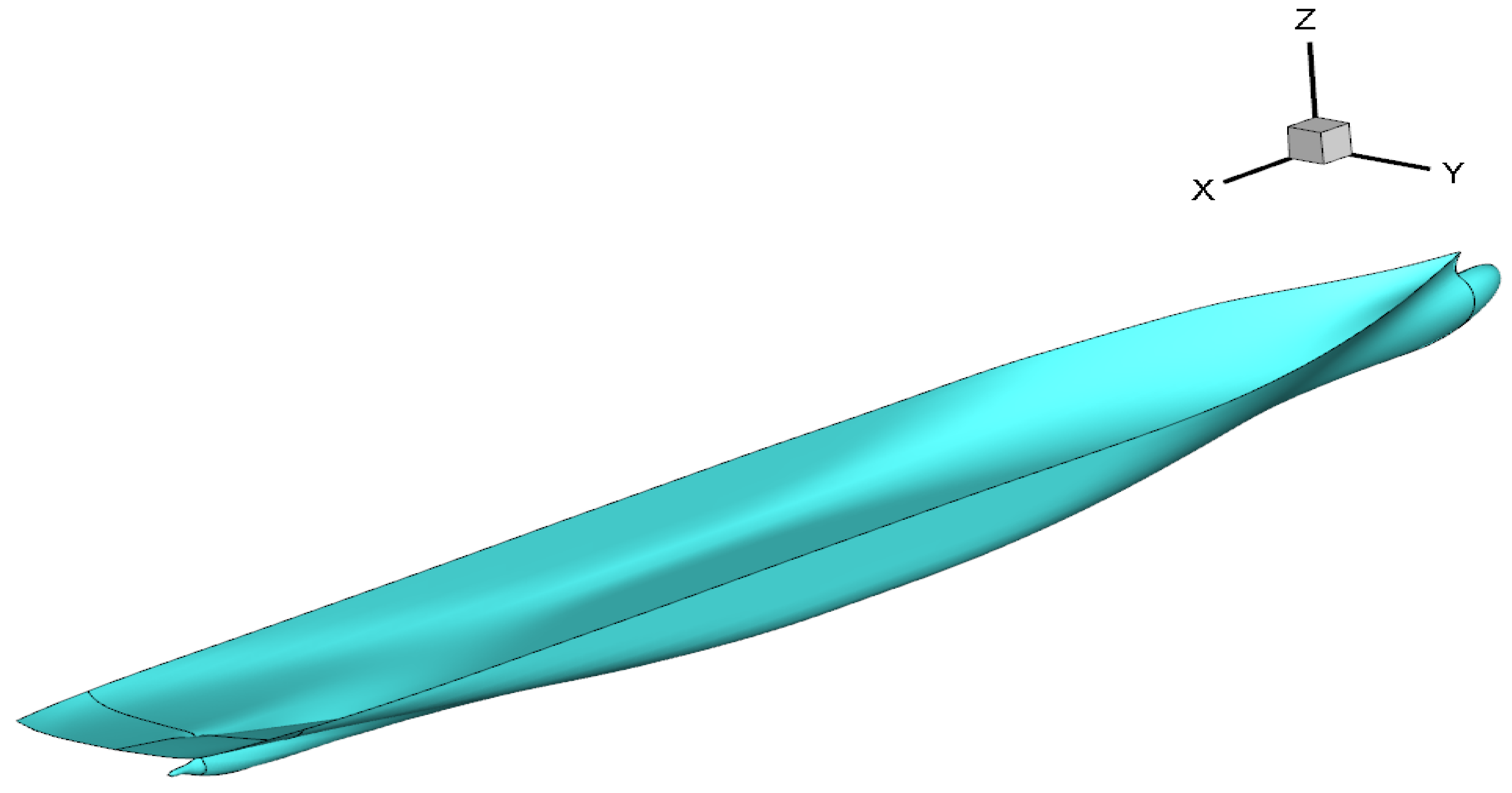
Figure 1.
Duisburg Test Case hull.

Figure 2.
DTC—domain and boundary conditions.

Figure 3.
Box refinement for wave capturing.

Figure 4.
Grid network for: (a) SHIPFLOW; (b) NUMECA/ANSYS.


Figure 5.
Comparison of total resistance between NUMECA, ANSYS and SHIPFLOW simulations.

Figure 6.
Force on the X-axis for all speeds computed.

Figure 7.
Trim for all speeds computed.

Figure 8.
Sinkage for all speeds computed.

Figure 9.
Wave height generated for all speeds—perspective view (Tecplot): (a) v = 1.335 m/s; (b) v = 1.401 m/s; (c) v = 1.469 m/s; (d) v = 1.535 m/s; (e) v = 1.602 m/s; (f) v = 1.668 m/s.
Figure 9.
Wave height generated for all speeds—perspective view (Tecplot): (a) v = 1.335 m/s; (b) v = 1.401 m/s; (c) v = 1.469 m/s; (d) v = 1.535 m/s; (e) v = 1.602 m/s; (f) v = 1.668 m/s.

Figure 10.
Total pressure (N/ for all speeds (Tecplot): (a) v = 1.335 m/s; (b) v = 1.401 m/s; (c) v = 1.469 m/s; (d) v = 1.535 m/s; (e) v = 1.602 m/s; (f) v = 1.668 m/s.
Figure 10.
Total pressure (N/ for all speeds (Tecplot): (a) v = 1.335 m/s; (b) v = 1.401 m/s; (c) v = 1.469 m/s; (d) v = 1.535 m/s; (e) v = 1.602 m/s; (f) v = 1.668 m/s.

Figure 11.
Hydrodynamic pressure (N/ for all speeds (Tecplot).

Figure 12.
Comparison between model test and CFD simulation with SHIPFLOW: (a) frictional resistance; (b) frictional resistance coefficient; (c) total resistance coefficient.
Figure 12.
Comparison between model test and CFD simulation with SHIPFLOW: (a) frictional resistance; (b) frictional resistance coefficient; (c) total resistance coefficient.


Table 1.
Main characteristics of the Duisburg Test Case (DTC).
| Main Particulars | Units | Model | Full Scale |
|---|---|---|---|
| Length between perpendiculars | (m) | 5.976 | 355 |
| Waterline breadth | (m) | 0.859 | 51 |
| Draught midship | (m) | 0.244 | 14.5 |
| Trim angle | (°) | 0 | 0 |
| Volume displacement | (m3) | 0.827 | 173,467 |
| Block coefficient | (-) | 0.661 | 0.661 |
| Wetted surface | (m2) | 6.243 | 22,032 |
| Design speed | (knots) | 3.244 | 25 |
Table 2.
Percentage error between experimental test and each CFD simulation for Rt.
| v (m/s) | PE_NUMECA Simulation (%) | PE_ANSYS Simulation (%) | PE_SHIPFLOW Simulation k-ω SST (%) | PE_SHIPFLOW Simulation k-ω BSL (%) | PE_SHIPFLOW Simulation EASM (%) |
|---|---|---|---|---|---|
| 1.335 | 3.29% | 2.08% | 4.92% | 1.01% | 3.93% |
| 1.401 | 1.90% | 1.68% | 2.81% | 3.12% | 1.94% |
| 1.469 | 2.36% | 1.40% | 1.62% | 4.26% | 0.76% |
| 1.535 | 2.53% | 2.90% | 0.87% | 5.13% | 0.12% |
| 1.602 | 1.55% | 4.42% | 0.66% | 5.34% | 0.29% |
| 1.668 | 1.72% | 5.44% | 1.19% | 4.52% | 0.37% |
Table 3.
Percentage error between experimental test and CFD simulation with SHIPFLOW for the Frictional Resistance (Rf).
Table 3.
Percentage error between experimental test and CFD simulation with SHIPFLOW for the Frictional Resistance (Rf).
| v (m/s) | PE_Rf_k-ω SST (%) | PE_Rf_k-ω BSL (%) | PE_Rf_EASM (%) |
|---|---|---|---|
| 1.335 | 5.46% | 0.70% | 5.33% |
| 1.401 | 5.04% | 1.24% | 4.91% |
| 1.469 | 4.88% | 1.40% | 4.74% |
| 1.535 | 4.55% | 1.80% | 4.41% |
| 1.602 | 4.25% | 2.35% | 4.04% |
| 1.668 | 4.13% | 2.39% | 3.92% |
Table 4.
Percentage error between experimental test and CFD simulation with SHIPFLOW for Frictional Resistance Coefficient (Cf).
Table 4.
Percentage error between experimental test and CFD simulation with SHIPFLOW for Frictional Resistance Coefficient (Cf).
| v (m/s) | PE_Cf_k-ω SST (%) | PE_Cf_k-ω BSL (%) | PE_Cf_EASM (%) |
|---|---|---|---|
| 1.335 | 2.46% | 3.88% | 2.37% |
| 1.401 | 2.04% | 4.46% | 1.88% |
| 1.469 | 1.86% | 4.62% | 1.73% |
| 1.535 | 1.55% | 5.01% | 1.39% |
| 1.602 | 1.24% | 5.57% | 1.01% |
| 1.668 | 1.08% | 5.64% | 0.89% |
Table 5.
Percentage error between experimental test and CFD simulation with SHIPFLOW for Total Resistance Coefficient (Ct).
Table 5.
Percentage error between experimental test and CFD simulation with SHIPFLOW for Total Resistance Coefficient (Ct).
| v (m/s) | PE_Ct_k-ω SST (%) | PE_Ct_k-ω BSL (%) | PE_Ct_EASM (%) |
|---|---|---|---|
| 1.335 | 1.88% | 0.90% | 0.90% |
| 1.401 | 0.28% | 1.17% | 1.17% |
| 1.469 | 1.48% | 2.40% | 2.40% |
| 1.535 | 2.28% | 3.30% | 3.30% |
| 1.602 | 2.48% | 3.48% | 3.48% |
| 1.668 | 1.93% | 2.78% | 2.78% |
Publisher’s Note: MDPI stays neutral with regard to jurisdictional claims in published maps and institutional affiliations. |
© 2021 by the authors. Licensee MDPI, Basel, Switzerland. This article is an open access article distributed under the terms and conditions of the Creative Commons Attribution (CC BY) license (http://creativecommons.org/licenses/by/4.0/).
Share and Cite
MDPI and ACS Style
Chiroșcă, A.-M.; Rusu, L. Comparison between Model Test and Three CFD Studies for a Benchmark Container Ship. J. Mar. Sci. Eng. 2021, 9, 62. https://doi.org/10.3390/jmse9010062
AMA Style
Chiroșcă A-M, Rusu L. Comparison between Model Test and Three CFD Studies for a Benchmark Container Ship. Journal of Marine Science and Engineering. 2021; 9(1):62. https://doi.org/10.3390/jmse9010062
Chicago/Turabian StyleChiroșcă, Ana-Maria, and Liliana Rusu. 2021. "Comparison between Model Test and Three CFD Studies for a Benchmark Container Ship" Journal of Marine Science and Engineering 9, no. 1: 62. https://doi.org/10.3390/jmse9010062
Note that from the first issue of 2016, this journal uses article numbers instead of page numbers. See further details here.