Time-Rescaling of Dirac Dynamics: Shortcuts to Adiabaticity in Ion Traps and Weyl Semimetals


1
Department of Physics, University of Maryland, Baltimore County, Baltimore, MD 21250, USA
2
Instituto de Física ‘Gleb Wataghin’, Universidade Estadual de Campinas, Campinas 13083-859, São Paulo, Brazil
*
Author to whom correspondence should be addressed.
Entropy 2021, 23(1), 81; https://doi.org/10.3390/e23010081
Submission received: 22 December 2020
/
Revised: 5 January 2021
/
Accepted: 5 January 2021
/
Published: 8 January 2021
(This article belongs to the Special Issue Shortcuts to Adiabaticity)
Abstract
:Only very recently, rescaling time has been recognized as a way to achieve adiabatic dynamics in fast processes. The advantage of time-rescaling over other shortcuts to adiabaticity is that it does not depend on the eigenspectrum and eigenstates of the Hamiltonian. However, time-rescaling requires that the original dynamics are adiabatic, and in the rescaled time frame, the Hamiltonian exhibits non-trivial time-dependence. In this work, we show how time-rescaling can be applied to Dirac dynamics, and we show that all time-dependence can be absorbed into the effective potentials through a judiciously chosen unitary transformation. This is demonstrated for two experimentally relevant scenarios, namely for ion traps and adiabatic creation of Weyl points.
1. Introduction
From the very beginning of quantum control, it has been recognized that circumventing the quantum adiabatic theorem [1] poses a formidable challenge. In essence, this theorem asserts that any quantum process that is driven at rates larger than the typical energy gaps, is inevitably accompanied by excitations [2,3,4,5]. In the real world, these parasitic excitations are often not only undesirable, but even detrimental. For instance, in adiabatic quantum computing [6], finite-time effects constitute a major source for computational errors [7,8]. Thus, to circumvent, mitigate, and suppress such finite-time excitations in controlled quantum processes, a wide variety of techniques has been developed. Among the most successful approaches are transitionless quantum driving [9,10,11,12,13], the fast-forward technique [14,15,16,17], and methods that rely on identifying the adiabatic invariants [18,19,20,21], to name just a few. For a comprehensive exposition of the field “shortcuts to adiabaticity”, we refer to recent reviews [22,23], a special collection of articles [24], and a perspective [25].
Somewhat naturally, the majority of work has focused on quantum processes that can be described by time-dependent Schrödinger equations. However, shortcuts to adiabaticty have also found generalizations and applications in, e.g., open system dynamics [26], classical dynamics [27,28], and even biologically relevant settings [29]. Complementing these efforts, the present paper focuses on relativistic quantum dynamics. This is motivated by recent work that has generalized the fast-forward technique [30], transitionless quantum driving [31], and invariant based methods [32] to controlled Dirac dynamics.
The Dirac equation [33] was originally formulated to describe the properties of massive spin- particles, such as electrons and quarks [34,35]. However, in recent years, it has attracted wider attention [36,37,38,39,40,41,42,43], which is mostly motivated by the discovery of so-called Dirac materials [44]. In these systems, the dispersion relation becomes linear, and hence the low-energy excitations behave more akin to massless Dirac particles than fermionic Schrödinger particles.
In the context of shortcuts to adiabaticity, the technical challenges already present for Schrödinger dynamics become significantly more involved for Dirac dynamics [45]. One way or another, implementing most shortcuts requires knowledge of the energy spectrum, or the use of highly non-local control fields. Therefore, any technique that requires less detailed information about the dynamics appears highly desirable [25]. In the following, we propose and demonstrate how the method of “time-rescaling” [46] is generalized to Dirac dynamics. We will see that, while simply applying a scaling transformation is mathematically straight forward, the potential physical implementations are markedly less clear. This originates in the fact that rescaling time leads to an effectively time-dependent mass [46]. We will show how this can be remedied by a judiciously chosen unitary transformation of the Dirac equation. The experimental applicability of our findings is demonstrated for two relevant systems, namely for ion traps and adiabatic pumping in Weyl semimetals.
Due to the wide variety of concepts used in the following analysis, the narrative has been written as self-contained as possible. In Section 2, we summarize the main properties of the Dirac equation, and briefly review time-rescaling for Schrödinger dynamics. In Section 3, we develop the method of time-rescaling for general Dirac dynamics. Section 4 is dedicated to adiabatically driving laser ion traps, and Section 5 presents adiabatic pumping in Weyl semimetals. Finally, the analysis is concluded with a few remarks in Section 6.
2. Preliminaries
We start by outlining notions and notations, and by briefly reviewing instrumental results from the literature.
2.1. Relativistic Quantum Mechanics: The Dirac Equation
The Dirac equation has its origin in an attempt to reconcile special relativity and quantum mechanics [33]. In its original inception and in first quantization, it correctly describes the properties of massive spin- particles. It can be written in space representation as [34],
Here, , the 4-dimensional Dirac spinor, i.e., the wave function of a charged spin- particle with rest mass m at position , and c is the speed of light. As usual, we denote the derivative with respect to time by a dot.
The -matrices are commonly written in terms of sub-matrices with the Pauli-matrices and the identity as,
Finally, is the vector potential, and is the scalar potential. The electric and magnetic fields, and , are given by
Note that the Dirac equation is gauge invariant [35], and we can thus choose mathematically convenient representations.
In the following, it will also prove convenient to introduce the Dirac–Hamiltonian , with which Equation (1) can be expressed in basis-independent form,
Hence, the Dirac Equation (5) becomes formally identical to the time-dependent Schrödinger equation. It is worth emphasizing, however, that the standard Schrödinger Hamiltonian is quadratic in momentum, whereas the Dirac–Hamiltonian is linear. This is a direct consequence of the relativistic energy–momentum relation, and it will become instrumental in the following analysis. Moreover, for massive particles, the Dirac–Hamiltonian contains the rest energy, which is not present in pure spin systems or in Schrödinger dynamics. We will see in the following that when rescaling time, this additional term requires special attention.
2.2. Time-Rescaling of Schrödinger Dynamics
Time-rescaling was put forward by Bernardo in Ref. [46] as an alternative method for finding shortcuts to adiabaticity, that does not depend on the instantaneous eigenstates of the dynamics. To this end, Ref. [46] considers the time-dependent Schrödinger equation
where is the standard Hamiltonian. The solution of Equation (6) can be expressed in terms of the unitary evolution operator,
where denotes time-ordering.
Time-rescaling is then nothing else but a transformation of the time variable in the exponent of the unitary evolution. We have
where is an arbitrary rescaling function. It is then easy to see that Equation (8) can be exploited as a shortcut to adiabaticity for any . If the original dynamics (7) describes an adiabatic process, then Equation (8) achieves the same adiabatic dynamics in shorter time, for all rescaling functions that obey the boundary conditions
where determines the “time contraction factor” [46].
The shortcoming of this technique is that in rescaled variables, the new Hamiltonian becomes . Generically, this leads to a time-dependent mass, which is not easy to realize in experimental scenarios. In Appendix A, we show how this can be remedied with the help of a canonical transformation. In particular, we show that time-rescaling and counterdiabetic driving are equivalent for scale-invariant problems [13].
3. Time-Rescaling of Dirac Dynamics
It is easy to see that the solution of the time-dependent Dirac Equation (5) can be expressed as
Hence, the time-rescaled dynamics become
where is the time-rescaled Dirac–Hamiltonian.
Hence, it appears to be rather straightforward to employ time-rescaling as a shortcut to adiabaticity also in Dirac dynamics. That the situation is not quite that simple becomes apparent when inspecting the explicit form of the Dirac–Hamiltonian (1). Notice, that while time-rescaling Schrödinger dynamics only led to a time-dependent mass, for Dirac dynamics, the time-scaled Hamiltonian is governed by an effectively time-dependent speed of light, , and an effectively time-dependent rest energy .
We will see in the following Section 4 that considering and is perfectly reasonable and realizable in ion traps, which are described by an effective Dirac equation. In general, however, it seems rather implausible that the speed of light and the rest energy can be considered time-dependent control parameters. Thus, we continue the analysis by proposing a canonical transformation that maps the effective time dependence exclusively onto vector and scalar potential, and .
For the sake of simplicity, and without loss of generality, we continue by considering a system that is restricted to the x-direction. In this case, the 4-component Dirac spinor can be separated into two identical 2-component bispinors. For mathematical convenience, we choose a representation in which the -dimensional Dirac equation reads [47,48],
and where we introduced the time-rescaled potentials and .
Absorbing the Time-Dependence into the Potentials
Our goal is now to find a unitary transformation that allows one to write the time-rescaled Hamiltonian in standard form, i.e., with time-independent speed of light and rest mass. Arguably, the simplest ansatz is given by
Thus, we obtain
and the corresponding solution is given by . We immediately observe that the time-dependent rest energy is multiplied by , whereas the kinetic term is modified by . Therefore, the two effectively time-dependent quantities, and , can be fully described by and its derivative , respectively.
We start by choosing
for which the rest energy becomes time-independent. In complete analogy to the Schrödinger case [46], the time-dependence of the kinetic term can then be absorbed into the vector potential. In particular, we define
which is nothing else but expressed in the corresponding interaction picture, plus a position-independent term.
Thus, we are only left with the pseudoscalar term [49,50], that is proportional to . Pseudoscalar potentials correspond physically to driving the system with circularly polarized light. Now, defining a new (scalar) potential
we finally obtain
where all the time dependence has been absorbed into the potentials. At first glance, the momentum-dependent vector potential may look unphysical. However, this is simply a consequence of the fact that the system is non-conservative, and hence the driven system will experience an intertial force [51], due to the “acceleration” from the time-rescaling.
In conclusion, we have shown that, while in Dirac dynamics we have two, instead of only one, effectively time-dependent parameters, a simple unitary transformation allows to absorb the time-dependence entirely into vector and scalar potentials. The resulting vector potential is fully analogous to what was proposed in Ref. [46] for Schrödinger dynamics, and the scalar potential contains a simple pseudoscalar term.
4. Dirac Dynamics in Laser Ion-Traps
It has been experimentally demonstrated that under certain conditions ions in laser traps can be described by effective Dirac dynamics [52,53,54,55]. In general, the applied laser field couples internal vibrational levels of the ion and its motional degrees of freedom. Hence, the total Hamiltonian reads,
where and describe motional and electronic degrees of freedom, respectively.
The interaction Hamiltonian can be written in (1 + 1) dimensions as [53]
where is the Lamb–Dicke parameter, m denotes the mass of the trapped ion, and is the axial frequency of the confining Paul trap. Note that the effective interaction can be tuned by applying an external magnetic field described by . Furthermore, and is the width the ground-state wave-function, and is the strength of the interaction, which is varied by modulating the laser source. Finally, describes the detuning of the laser and the resonance frequency of the two-level atom. In principle, both and can be controlled externally, and varied as a function of time.
Hence, is already in the time-dependent form required to implement a shortcut to adiabaticity by means of time-rescaling.
A Simple Demonstration
Before we continue, it is instructive to demonstrate time-rescaled Dirac dynamics in ion traps with a simple example. To this end, consider a simple scenario, in which we again choose . In the interaction picture, we have
Note that the latter Hamiltonian is written in instantaneous units of . Thus, we simply have and . Its instantaneous eigenstates can be expressed as
where and are basis states of and , where is the instantaneous momentum. We immediately observe that for large enough , this simple Dirac–Hamiltonian (22) describes adiabatic dynamics, i.e., a system prepared in an initial eigenstate will remain in the corresponding, instantaneous eigenstate.
Now let us assume that the desired target state of the dynamics is , which is the instantaneous eigenstate of at . Using time-rescaling, this target state can be reached in a shorter time. To this end, we choose the rescaling function [46] to read
where as before, is the acceleration factor. It is easy to see [46] that this choice fulfills all boundary conditions (9), and notice that, for , we simply have , i.e., we recover the original dynamics.
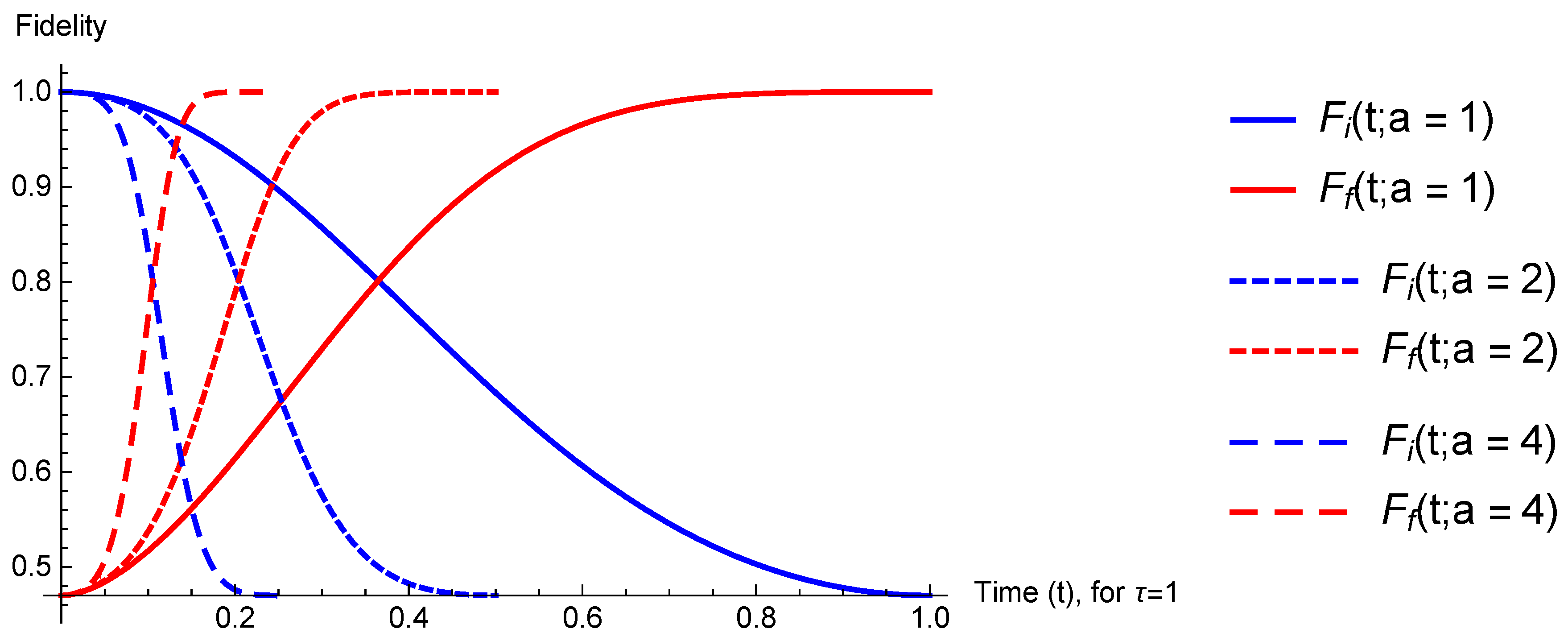
It is then a simple exercise to solve the dynamics numerically for the original Hamiltonian, , (22) and its time-rescaled companion, . To illustrate our findings, we choose the system to be initially prepared in (23), and compute the fidelity of the time-evolved state with respect to initial and target state, and , respectively. These are given by
In Figure 1, we depict the fidelities for a range of values of a. As expected, we see that for , the target state is reached in time .
5. Time-Rescaling Weyl Semimetals: Shortcuts to Adiabatic Pumping
As a second example we discuss time rescaling in the context of adiabatic pumping for Weyl semimetals. To this end, we need to apply the above developed framework to Floquet theory, first.
5.1. Floquet Theory and Time-Rescaling
The solution of periodically driven many-body Hamiltonians can be expanded in the so-called Floquet states [56]. To this end, consider a general Hamiltonian [57],
where k is the wave vector in the first Brilloin zone. Here, a and are the fermionic annihilation and creation operators, and n and m are indices associated with the system’s degrees of freedom. If this Hamiltonian is periodic in time, , the single particle wave function can be written as [56,58],
where is the Floquet mode with periodicity T. The quasienergies are eigenvalues of the Floquet operator equation, and they satisfy,
Hence, the exhibit the corresponding Floquet band structure, if the are also periodic in momentum space. Interestingly, for fermionic systems, Floquet theories predict a variety of topological states of matter [57], which we will be exploiting in the following.
The major advantage of the Floquet ansatz (27) is that the time evolution operator can be factorized. We have [59],
and . Thus, it is not difficult to realize that time rescaling can be used to shorten the periodicity of the solutions, and in particular, we can write
where, as above, s is the re-scaled time variable and is the re-scaling function.
If we again consider time acceleration, i.e., for , then the periodicity of the Floquet states is shorted by a factor of . In the following, we will exploit this observation for adiabatic evolution between Floquet points, or in other words, will we use time rescaling as a shortcut to adiabatic pumping.
In this context, it is also interesting to note that typically, a periodically driven Hamiltonian does not have to be periodic in momentum space. However, it is still possible to introduce the Floquet operator in terms of a periodic momentum transport variable [60]. Experimentally, this transport variable can be manifested by phase-shifting two optical-lattice potentials in a ratchet accelerator (RA) model [60], and its infinitesimal evolution corresponds to tracing out the entire Floquet band topology, by moving between different eigenstates of the Floquet operator.
5.2. Shortcut to Adiabatic Creation of Weyl Points
Only rather recently, it has been shown that Floquet points can exhibit linear dispersion relations. For instance, Refs. [61,62] found topological phases that correspond to Weyl semimetals with three-dimensional Dirac “cones”. This was achieved, by considering a modified, extended kicked Harper model and the careful tuning of “hopping” and “kicking” strengths.
We will now briefly outline how time-rescaling can be applied to create these Weyl points in Floquet theory in shorter time. To this end, we consider the off-diagonal kicked Harper model, whose Hamiltonian reads [62]
where n is the lattice site index, J and are parameters controlling the hopping strength, N is the total number of lattice sites. Furthermore, is the onsite potential, represents the coupling with the harmonic driving field, and . As before, T is the period of driving, and . In this model [62], and are quasimomenta, that can take any value in . Therefore, we can simplify the analysis again to (1 + 1) dimensions. It is also interesting to note, that Weyl chirality can be manifested by observing the time evolution of the mean position, . This is facilitated by adiabatic transport in momentum space [60], or rather by the adiabatic variation of and . Thus, we focus now on applying time rescaling for adiabatic transport to observe the Weyl chirality in .
It can be shown that the corresponding quasienergy spectrum exhibits band touching points with linear dispersion relation [61,62].
For the time-dependent variation of and , Equation (32) can be written as [62]
where . The corresponding time-rescaled Hamiltonian becomes, , and we now need to verify that also exhibits the desired Weyl chirality.
Moreover, we have , , , and . Finally, ℓ denotes the quantum number of the quasienergy. Adiabatic momentum transport is then achieved by parametrizing and according to and and evolving over a time period [62]. Thus, it is worth emphasizing that the relevant Floquet operator quantifies this periodicity, , in momentum space, and not the time period of the driving field T.
Solving for the time evolution operator exactly is hardly feasible. However, the Floquet operator (29) can be obtained from time-dependent perturbation theory. It can be shown [62] that we have for the first period
where is the Bessel function of the first kind. It is then a simple exercise to show that we obtain for the time-rescaled Floquet operator
which is identical to the Floquet operator (36). However, due to time rescaling, has a periodicity of , which for , described sped-up dynamics. Since the time-rescaled Floquet operator is identical to the original , all further steps of the analysis in Ref. [62] remain true, yet the Weyl chirality is obtained with periodicity .
Finally, we briefly remark on the complexity of the time-dependence in the time-rescaled dynamics. As before, in , all original parameters are multiplied by . In particular, this requires both kicking and hopping strengths to be varied with time. However, it is not hard to see that, in complete analogy to the above in Section 3, the time dependence can be absorbed into potentials. This can be facilitated again with, e.g., the simplest unitary transformation (13).
6. Concluding Remarks
Controlling quantum systems is a ubiquitous goal in the development of quantum technologies. To this end, shortcuts to adiabaticity provide a powerful tool kit to steer quantum system towards desired target states. However, most techniques are rather complicated to be implemented in realistic scenarios, since most of them require exquisite knowledge about the eigenspectrum of the driven Hamiltonians.
Time scaling relies on the simple idea that, rather than controlling single states, faster dynamics can be achieved by simply transforming the dynamics to a new time-frame. To utilize time rescaling as a shortcut to adiabaticty, two criteria need to me met: (i) the original dynamics is adiabatic, and (ii) the resulting Hamiltonian has to be realizable and physical.
Using time rescaling as a shortcut was originally proposed only for Schrödinger dynamics. The natural question arose, whether also relativistic dynamics can be treated in this framework. To answer this question, we have analyzed Dirac dynamics in first quantization. In the second quantization, one has to be concerned with pair production and radiation, and hence a quantum field theoretic description becomes inevitable.
In the present paper, we have shown that time-rescaling can be directly applied to Dirac dynamics, and that the aforementioned criteria are met by at least two experimentally relevant scenarios, namely laser ion traps and the adiabatic creation of Weyl points. Thus, we remain optimistic that time-rescaling will, indeed, find applications in experimental settings.
Author Contributions
Conceptualization, A.R. and S.D.; formal analysis, A.R. and S.D.; writing—original draft preparation, A.R. and S.D.; writing—review and editing, A.R. and S.D.; funding acquisition, S.D. All authors have read and agreed to the published version of the manuscript.
Funding
This research was supported by grant number FQXi-RFP-1808 from the Foundational Questions Institute and Fetzer Franklin Fund, a donor-advised fund of Silicon Valley Community Foundation (SD).
Acknowledgments
ARC thanks Pierre Nazé for bringing Ref. [46] to our attention. Enlightening discussions with Akram Touil and Nirnoy Basak are gratefully acknowledged.
Conflicts of Interest
The authors declare no conflict of interest.
Appendix A. Shortcuts to Adiabaticity from Time Rescaling in Scale Invariant Problems
This appendix is dedicated to the question of whether time-rescaling is related to, or even equivalent to, other techniques for shortcuts to adiabaticity. To this end, we analyze the method for scale-invariant problems, in both classical and quantum dynamics.
Appendix A.1. Classical Hamiltonian Dynamics
We start by considering a classical system that evolves under Hamiltonian, scale-invariant dynamics. For such problems, it has been shown that the counterdiabatic field facilitating transitionless quantum driving takes a particularly simple form [13].
The corresponding Hamiltonian is given by
where m is the mass of the particle, = and V are the scale-invariant driving potentials obeying . Note that time rescaling can be applied directly to classical dynamics, by replacing the commutator in the Heisenberg equation of motion with the Poisson bracket.
The corresponding time-rescaled Hamiltonian becomes
which has the same technical problem that we discussed in the main text, namely contains an effectively time-dependent mass. Scaling time is actually a well-studied problem in Hamiltonian dynamics, and it can be expressed in terms of an infinitesimal canonical transformation [63].
Therefore, we now consider a generating function of the second kind [64]
where and are two arbitrary functions of time. Accordingly, we have
Noting , it is then straightforward to show that
where and we suppressed the time-dependence of the parameters to avoid clutter.
Choosing the arbitrary functions and as
the non-local term disappears and the time-dependence of the kinetic terms is remedied. Hence, we can write
with .
In conclusion, we have shown that time-rescaling in scale-invariant problems is equivalent to including an auxiliary field, which is simply given by a harmonic term. Since it also has been shown that the counterdiabatic field in transitionless quantum driving can be reduced to a harmonic term [13], we have that time-rescaling can indeed facilitate transitionless quantum driving.
Appendix A.2. Scale-Invariant Schrödinger Dynamics
The analogous problem can also be solved for Schrödinger dynamics. In this case, we write the quantum generating function as
for two arbitrary functions and , and . Now choosing,
we obtain for
and . In complete analogy to the classical case, time-rescaling in the original frame is facilitated by an auxiliary harmonic term.
References
- Born, M. Das Adiabatenprinzip in der Quantenmechanik. Z. Phys. 1927, 40, 167. [Google Scholar] [CrossRef]
- Messiah, A. Quantum Mechanics; John Wiley & Sons: Amsterdam, The Netherlands, 1966; Volume 2. [Google Scholar]
- Nenciu, G. On the adiabatic theorem of quantum mechanics. J. Phys. A Math. Gen. 1980, 13, L15–L18. [Google Scholar] [CrossRef]
- Nenciu, G. On the adiabatic limit for Dirac particles in external fields. Commun. Math. Phys. 1980, 76, 117. [Google Scholar] [CrossRef]
- Nenciu, G. Adiabatic theorem and spectral concentration. Commun. Math. Phys. 1981, 82, 121. [Google Scholar] [CrossRef]
- Albash, T.; Lidar, D.A. Adiabatic quantum computation. Rev. Mod. Phys. 2018, 90, 015002. [Google Scholar] [CrossRef] [Green Version]
- Young, K.C.; Sarovar, M.; Blume-Kohout, R. Error Suppression and Error Correction in Adiabatic Quantum Computation: Techniques and Challenges. Phys. Rev. X 2013, 3, 041013. [Google Scholar] [CrossRef] [Green Version]
- Gardas, B.; Deffner, S. Quantum fluctuation theorem for error diagnostics in quantum annealers. Sci. Rep. 2018, 8, 17191. [Google Scholar] [CrossRef]
- Demirplak, M.; Rice, S.A. Adiabatic Population Transfer with Control Fields. J. Chem. Phys. A 2003, 107, 9937. [Google Scholar] [CrossRef]
- Demirplak, M.; Rice, S.A. Assisted adiabatic passage revisited. J. Phys. Chem. B 2005, 109, 6838. [Google Scholar] [CrossRef]
- Berry, M. Transitionless quantum driving. J. Phys. A Math. Theor. 2009, 42, 365303. [Google Scholar] [CrossRef] [Green Version]
- Del Campo, A. Shortcuts to Adiabaticity by Counterdiabatic Driving. Phys. Rev. Lett. 2013, 111, 100502. [Google Scholar] [CrossRef] [PubMed] [Green Version]
- Deffner, S.; Jarzynski, C.; del Campo, A. Classical and quantum shortcuts to adiabaticity for scale-invariant driving. Phys. Rev. X 2014, 4, 021013. [Google Scholar] [CrossRef] [Green Version]
- Masuda, S.; Nakamura, K. Fast-forward of adiabatic dynamics in quantum mechanics. Proc. R. Soc. A 2010, 466, 1135. [Google Scholar] [CrossRef]
- Masuda, S.; Nakamura, K. Acceleration of adiabatic quantum dynamics in electromagnetic fields. Phys. Rev. A 2011, 84, 043434. [Google Scholar] [CrossRef]
- Masuda, S.; Rice, S.A. Fast-Forward Assisted STIRAP. J. Phys. Chem. A 2015, 119, 3479. [Google Scholar] [CrossRef] [Green Version]
- Masuda, S.; Nakamura, K.; Nakahara, M. Fast-forward scaling theory for phase imprinting on a BEC: Creation of a wave packet with uniform momentum density and loading to Bloch states without disturbance. New J. Phys. 2018, 20, 025008. [Google Scholar] [CrossRef]
- Chen, X.; Ruschhaupt, A.; Schmidt, S.; del Campo, A.; Guéry-Odelin, D.; Muga, J.G. Fast Optimal Frictionless Atom Cooling in Harmonic Traps: Shortcut to Adiabaticity. Phys. Rev. Lett. 2010, 104, 063002. [Google Scholar] [CrossRef]
- Torrontegui, E.; Martínez-Garaot, S.; Muga, J.G. Hamiltonian engineering via invariants and dynamical algebra. Phys. Rev. A 2014, 89, 043408. [Google Scholar] [CrossRef] [Green Version]
- Kiely, A.; McGuinness, J.P.L.; Muga, J.G.; Ruschhaupt, A. Fast and stable manipulation of a charged particle in a Penning trap. J. Phys. B At. Mol. Opt. Phys. 2015, 48, 075503. [Google Scholar] [CrossRef] [Green Version]
- Jarzynski, C.; Deffner, S.; Patra, A.; Subaşı, Y.B.U. Fast forward to the classical adiabatic invariant. Phys. Rev. E 2017, 95, 032122. [Google Scholar] [CrossRef] [Green Version]
- Torrontegui, E.; Ibáñez, S.; Martínez-Garaot, S.; Modugno, M.; del Campo, A.; Guéry-Odelin, D.; Ruschhaupt, A.; Chen, X.; Muga, J.G. Shortcuts to Adiabaticity. Adv. At. Mol. Opt. Phys. 2013, 62, 117. [Google Scholar] [CrossRef] [Green Version]
- Guéry-Odelin, D.; Ruschhaupt, A.; Kiely, A.; Torrontegui, E.; Martínez-Garaot, S.; Muga, J.G. Shortcuts to adiabaticity: Concepts, methods, and applications. Rev. Mod. Phys. 2019, 91, 045001. [Google Scholar] [CrossRef]
- Del Campo, A.; Kim, K. Focus on Shortcuts to Adiabaticity. New J. Phys. 2019, 21, 050201. [Google Scholar] [CrossRef]
- Deffner, S.; Bonança, M.V.S. Thermodynamic control—An old paradigm with new applications. EPL (Europhys. Lett.) 2020, 131, 20001. [Google Scholar] [CrossRef]
- Alipour, S.; Chenu, A.; Rezakhani, A.T.; del Campo, A. Shortcuts to Adiabaticity in Driven Open Quantum Systems: Balanced Gain and Loss and Non-Markovian Evolution. Quantum 2020, 4, 336. [Google Scholar] [CrossRef]
- Patra, A.; Jarzynski, C. Classical and Quantum Shortcuts to Adiabaticity in a Tilted Piston. J. Phys. Chem. B 2017, 121, 3403–3411. [Google Scholar] [CrossRef] [PubMed] [Green Version]
- Patra, A.; Jarzynski, C. Shortcuts to adiabaticity using flow fields. New J. Phys. 2017, 19, 125009. [Google Scholar] [CrossRef]
- Iram, S.; Dolson, E.; Chiel, J.; Pelesko, J.; Krishnan, N.; Güngör, Ö.; Kuznets-Speck, B.; Deffner, S.; Ilker, E.; Scott, J.G.; et al. Controlling the speed and trajectory of evolution with counterdiabatic driving. Nat. Phys. 2020. [Google Scholar] [CrossRef]
- Deffner, S. Shortcuts to adiabaticity: Suppression of pair production in driven Dirac dynamics. New J. Phys. 2015, 18, 012001. [Google Scholar] [CrossRef]
- Fan, Q.Z.; Cheng, X.H.; Chen, X. Counter-diabatic driving for Dirac dynamics. In Young Scientists Forum 2017; Zhuang, S., Chu, J., Pan, J.W., Eds.; International Society for Optics and Photonics, SPIE: Philadelphia, PA, USA, 2018; Volume 10710, pp. 42–47. [Google Scholar] [CrossRef]
- Song, X.K.; Deng, F.G.; Lamata, L.; Muga, J.G. Robust state preparation in quantum simulations of Dirac dynamics. Phys. Rev. A 2017, 95, 022332. [Google Scholar] [CrossRef] [Green Version]
- Dirac, P.A.M. The quantum theory of the electron. Proc. R. Soc. A 1928, 117, 778. [Google Scholar] [CrossRef] [Green Version]
- Thaller, B. The Dirac Equation; Springer: Berlin, Germany, 1956. [Google Scholar]
- Peskin, M.E.; Schroeder, D.V. An Introduction to Quantum Field Theory (Frontiers in Physics); Westview Press: Boulder, CO, USA, 1995. [Google Scholar]
- Pickl, P.; Dürr, D. On Adiabatic Pair Creation. Commun. Math. Phys. 2008, 282, 161. [Google Scholar] [CrossRef] [Green Version]
- Fillion-Gourdeau, F.; Lorin, E.; Bandrauk, A.D. Landau-Zener-Stückelberg interferometry in pair production from counterpropagating lasers. Phys. Rev. A 2012, 86, 032118. [Google Scholar] [CrossRef] [Green Version]
- Fillion-Gourdeau, F.; Lorin, E.; Bandrauk, A.D. Resonantly Enhanced Pair Production in a Simple Diatomic Model. Phys. Rev. Lett. 2013, 110, 013002. [Google Scholar] [CrossRef] [PubMed] [Green Version]
- Fillion-Gourdeau, F.; Lorin, E.; Bandrauk, A.D. Enhanced Schwinger pair production in many-centre systems. J. Phys. B At. Mol. Opt. Phys. 2013, 46, 175002. [Google Scholar] [CrossRef] [Green Version]
- Fillion-Gourdeau, F.; MacLean, S. Time-dependent pair creation and the Schwinger mechanism in graphene. Phys. Rev. B 2015, 92, 035401. [Google Scholar] [CrossRef]
- Villamizar, D.V.; Duzzioni, E.I. Quantum speed limit for a relativistic electron in a uniform magnetic field. Phys. Rev. A 2015, 92, 042106. [Google Scholar] [CrossRef] [Green Version]
- Schmidt, M.; Peano, V.; Marquardt, F. Optomechanical Dirac physics. New J. Phys. 2015, 17, 023025. [Google Scholar] [CrossRef] [Green Version]
- Deffner, S.; Saxena, A. Quantum work statistics of charged Dirac particles in time-dependent fields. Phys. Rev. E 2015, 92, 032137. [Google Scholar] [CrossRef] [Green Version]
- Wehling, T.O.; Black-Schaffer, A.M.; Balatsky, A.V. Dirac materials. Adv. Phys. 2014, 63, 1. [Google Scholar] [CrossRef] [Green Version]
- Faisal, F.H.M. Adiabatic solutions of a Dirac equation of a new class of quasi-particles and high harmonic generation from them in an intense electromagnetic field. J. Phys. B At. Mol. Opt. Phys. 2011, 44, 111001. [Google Scholar] [CrossRef]
- Bernardo, B.d.L. Time-rescaled quantum dynamics as a shortcut to adiabaticity. Phys. Rev. Res. 2020, 2, 013133. [Google Scholar] [CrossRef] [Green Version]
- De Castro, A.S. Bound states by a pseudoscalar Coulomb potential in one-plus-one dimensions. Phys. Lett. A 2003, 318, 40. [Google Scholar] [CrossRef] [Green Version]
- Solomon, D. An exact solution of the Dirac equation for a time-dependent Hamiltonian in 1-1 dimension space-time. Can. J. Phys. 2010, 88, 137. [Google Scholar] [CrossRef] [Green Version]
- Haouat, S.; Chetouani, L. The (1+1)-Dimensional Dirac Equation with Pseudoscalar Potentials: Path Integral Treatment. Int. J. Theo. Phys. 2007, 46, 1528. [Google Scholar] [CrossRef]
- Haouat, S.; Chetouani, L. The (1+1)-dimensional Dirac equation with pseudoscalar potentials: Quasi-classical approximation. Phys. Scri. 2008, 78, 065005. [Google Scholar] [CrossRef]
- Gardas, B.; Deffner, S.; Saxena, A. Repeatability of measurements: Non-Hermitian observables and quantum Coriolis force. Phys. Rev. A 2016, 94, 022121. [Google Scholar] [CrossRef] [Green Version]
- Leibfried, D.; Blatt, R.; Monroe, C.; Wineland, D. Quantum dynamics of single trapped ions. Rev. Mod. Phys. 2003, 75, 281–324. [Google Scholar] [CrossRef] [Green Version]
- Lamata, L.; León, J.; Schätz, T.; Solano, E. Dirac Equation and Quantum Relativistic Effects in a Single Trapped Ion. Phys. Rev. Lett. 2007, 98, 253005. [Google Scholar] [CrossRef] [Green Version]
- Gerritsma, R.; Kirchmair, G.; Zähringer, F.; Solano, E.; Blatt, R.; Roos, C.F. Quantum simulation of the Dirac equation. Nature 2010, 463, 68–71. [Google Scholar] [CrossRef] [Green Version]
- Muga, J.G.; Simón, M.A.; Tobalina, A. How to drive a Dirac system fast and safe. New J. Phys. 2016, 18, 021005. [Google Scholar] [CrossRef] [Green Version]
- Floquet, G. Sur les équations différentielles linéaires à coefficients périodiques. Ann. Sci. l’École Norm. Supérieure 1883, 12, 47–88. [Google Scholar] [CrossRef] [Green Version]
- Lindner, N.H.; Refael, G.; Galitski, V. Floquet topological insulator in semiconductor quantum wells. Nat. Phys. 2011, 7, 490–495. [Google Scholar] [CrossRef] [Green Version]
- Shirley, J.H. Solution of the Schrödinger Equation with a Hamiltonian Periodic in Time. Phys. Rev. 1965, 138, B979–B987. [Google Scholar] [CrossRef]
- Dittrich, T.; Hänggi, P.; Ingold, G.L.; Kramer, B.; Schön, G.; Zwerger, W. Quantum Transport and Dissipation; Wiley-VCH: Weinheim, Germany, 1998. [Google Scholar]
- Ho, D.Y.H.; Gong, J. Quantized Adiabatic Transport In Momentum Space. Phys. Rev. Lett. 2012, 109, 010601. [Google Scholar] [CrossRef] [Green Version]
- Bomantara, R.W.; Raghava, G.N.; Zhou, L.; Gong, J. Floquet topological semimetal phases of an extended kicked Harper model. Phys. Rev. E 2016, 93, 022209. [Google Scholar] [CrossRef] [Green Version]
- Bomantara, R.W.; Gong, J. Generating controllable type-II Weyl points via periodic driving. Phys. Rev. B 2016, 94, 235447. [Google Scholar] [CrossRef] [Green Version]
- Carinena, J.F.; Ibort, L.A.; Lacomba, E.A. Time Scaling as an Infinitesimal Canonical Transformation. Celest. Mech. 1988, 42, 201–213. [Google Scholar] [CrossRef]
- Goldstein, H. Classical Mechanics; Addison-Wesley: Reading, MA, USA, 1980. [Google Scholar]
Figure 1.
Fidelity of the time-evolved state with respect to initial and target state (25) for and . Other parameters are set such that .
Figure 1.
Fidelity of the time-evolved state with respect to initial and target state (25) for and . Other parameters are set such that .

Publisher’s Note: MDPI stays neutral with regard to jurisdictional claims in published maps and institutional affiliations. |
© 2021 by the authors. Licensee MDPI, Basel, Switzerland. This article is an open access article distributed under the terms and conditions of the Creative Commons Attribution (CC BY) license (http://creativecommons.org/licenses/by/4.0/).
Share and Cite
MDPI and ACS Style
Roychowdhury, A.; Deffner, S. Time-Rescaling of Dirac Dynamics: Shortcuts to Adiabaticity in Ion Traps and Weyl Semimetals. Entropy 2021, 23, 81. https://doi.org/10.3390/e23010081
AMA Style
Roychowdhury A, Deffner S. Time-Rescaling of Dirac Dynamics: Shortcuts to Adiabaticity in Ion Traps and Weyl Semimetals. Entropy. 2021; 23(1):81. https://doi.org/10.3390/e23010081
Chicago/Turabian StyleRoychowdhury, Agniva, and Sebastian Deffner. 2021. "Time-Rescaling of Dirac Dynamics: Shortcuts to Adiabaticity in Ion Traps and Weyl Semimetals" Entropy 23, no. 1: 81. https://doi.org/10.3390/e23010081
Note that from the first issue of 2016, this journal uses article numbers instead of page numbers. See further details here.