Characteristics of Locally Occurring High PM2.5 Concentration Episodes in a Small City in South Korea


1
Department of Interdisciplinary Graduate Program in Environmental and Biomedical Convergence, Kangwon National University, Chuncheon, Gangwon-do 24341, Korea
2
Division of Chemical Research, National Institute of Environmental Research, Incheon 22689, Korea
3
Department of Environmental Science, Kangwon National University, Chuncheon, Gangwon-do 24341, Korea
*
Author to whom correspondence should be addressed.
Atmosphere 2021, 12(1), 86; https://doi.org/10.3390/atmos12010086
Submission received: 14 December 2020
/
Revised: 30 December 2020
/
Accepted: 5 January 2021
/
Published: 8 January 2021
(This article belongs to the Section Aerosols)
Abstract
:In this study, the ionic and carbonaceous compounds in PM2.5 were analysed in the small residential city of Chuncheon, Korea. To identify the local sources that substantially influence PM2.5 concentrations, the samples were divided into two groups: samples with PM2.5 concentrations higher than those in the upwind metropolitan area (Seoul) and samples with lower PM2.5 concentrations. During the sampling period (December 2016–August 2018), the average PM2.5 was 23.2 μg m−3, which exceeds the annual national ambient air quality standard (15 μg m−3). When the PM2.5 concentrations were higher in Chuncheon than in Seoul, the organic carbon (OC) and elemental carbon (EC) concentrations increased the most among all the PM2.5 components measured in this study. This is attributable to secondary formation and biomass burning, because secondary OC was enhanced and water soluble OC was strongly correlated with K+, EC, and OC. A principal component analysis identified four factors contributing to PM2.5: fossil-fuel combustion, secondary inorganic and organic reactions in biomass burning plumes, crustal dust, and secondary NH4+ formation.
1. Introduction
Particles less than 2.5 μm in diameter (PM2.5) contribute to many serious issues, including adverse effects on human health, deteriorating visibility, and transboundary transport. PM2.5 has also been reported to have direct and indirect effects on climate change, as the particles effectively scatter solar radiation and act as cloud condensation nuclei [1,2,3,4]. PM2.5 is emitted directly from anthropogenic (such as mobile sources, coal power plants, and biomass burning) and natural sources (such as sea salt, soil re-suspension, and volcanic eruptions) or is formed secondarily in the atmosphere through complex homo- and heterogeneous reactions [5,6]. These PM2.5 types are primary and secondary PM2.5, respectively. Many studies have identified possible sources and/or formation pathways of PM2.5 based on detailed chemical composition data [7,8,9]. PM2.5 mainly consists of water-soluble ionic compounds and organic and elemental carbon, with trace levels of metallic elements. Elemental carbon (EC) is emitted primarily by combustion processes [10,11,12,13,14]. On the other hand, organic carbon (OC) can be either directly emitted by both natural and anthropogenic sources or formed secondarily in the ambient air through homogeneous gas-phase oxidation, gas–aerosol partitioning, and/or heterogeneous oxidation of volatile organic compounds. In previous studies, secondary OC (SOC) has often been estimated using the EC tracer method [15,16,17]. OC can be classified into water-soluble OC (WSOC) and water-insoluble OC (WIOC). WSOC has been suggested as a proxy for SOC [18,19,20,21,22], but some studies have also indicated that WSOC is also emitted by non-fossil fuel combustion, including biomass combustion [23,24,25,26]. Previous studies have shown that approximately 50–80% of PM2.5 mass is secondary, mainly existing as NH4NO3, (NH4)2SO4, and various forms of OC [27,28].
PM2.5 has recently emerged as the most important air pollutant in South Korea, while concentrations of other representative pollutants, including SO2 and CO, have decreased steadily in recent decades. According to the 2018 World Air Quality Report by AirVisual [29], South Korea is second behind Chile among the organization for economic cooperation and development (OECD) countries, and 44 Korean cities are among the worst 100 cities. Approximately 98% of the sites in the National Monitoring Network of Air Quality exceeded the South Korean annual National Ambient Air Quality Standard (NAAQS) of 15 μg m−3. Since PM2.5 is a significant transboundary pollutant and due to South Korea’s proximity to China, the contributions of Chinese sources to PM2.5 concentrations in South Korea have been considered to be as large or larger than those of national sources [27,28,30,31].
In this study, we measured the atmospheric concentrations of PM2.5 and its ionic and carbonaceous compounds in the relatively small residential city of Chuncheon, South Korea. Chuncheon is located −100 km northeast of Seoul, South Korea. According to the National Emissions Inventory (2017), the PM2.5 emission rate from anthropogenic sources in Chuncheon is quite low (167.3 metric tons) compared to Seoul (1629.4 metric tons). However, PM2.5 concentrations in Chuncheon have often been similar to or higher than those in Seoul. Although the sources affecting PM2.5 concentrations in Chuncheon are considered to be different from the major source types in metropolitan and industrial cities, only a few studies have identified potential PM2.5 sources in small cities with low anthropogenic emissions [7,32]. Because westerly winds dominate this area, episodes of high PM2.5 concentrations in Chuncheon are presumed to be caused by regional and long-range transport from urban and industrial areas of Korea and China; therefore, there have been few attempts to identify local PM2.5 sources in the city. In addition, previous studies have identified PM2.5 sources using PM2.5 chemical compositions [33,34], relationships with other pollutants [35,36], and receptor modelling such as positive matrix factorisation (PMF) [37,38]; however, it is difficult to determine whether the identified source is local or whether it has been affected by long-range transport. In this study, PM2.5 samples were divided into two groups: PM2.5 concentrations that were higher and lower than those in the upwind area (Seoul). The characteristics of PM2.5 in these two groups and their major components were then compared.
2. Methods
2.1. Sample Collection
PM2.5 samples were collected on the roof of a 4 story building at Kangwon National University in Chuncheon, South Korea, from December 2016 to August 2018. Chuncheon is a small residential city with no large anthropogenic sources because the city has been designated as a water resource protected area. The city is located −100 km northeast of Seoul (the capital and largest city in South Korea) and is along the border of Gyeonggi Province, where various large industries are located. Therefore, air pollutants emitted by Seoul and the adjacent industrial areas are likely transported to Chuncheon by the prevailing westerly winds (Figure 1). Samples were collected for 24 h every 6 d from December 2016 to November 2017, and additional measurements were conducted when high PM2.5 concentrations were forecasted. From December 2017 to August 2018, samples were continuously collected over consecutive 71 h periods (for example, one sample was collected from 11 am on December 3 to 10 am on 6 December 2017). A 47 mm Teflon filter with a supported polypropylene ring (2.0 μm pore size, Pall Co., Port Washington, NY, USA) was used in a PMS-103 sampler (APM Engineering, Bucheon-si, Korea) at a flow rate of 16.7 L min−1 to determine the PM2.5 mass concentrations. A 47 mm quartz filter (2.2 μm pore size, Whatman International Ltd., Maidstone, UK) that was previously baked in a furnace at 500 °C for 24 h was used at a flow rate of 16.7 L min−1 to measure the carbonaceous compounds in the PM2.5. A carbon denuder was connected to the system between a cyclone and a filter pack to remove possible artefacts after February 2018.
To collect ionic compounds, a cyclone (URG-2000-30EN), two 3 channel annular denuders (242 mm length, URG Co., Chapel Hill, NC, USA), and a 3 stage Teflon filter pack (URG Co., Chapel Hill, NC, USA) were connected in sequence at a flow rate of 10 L min−1 to eliminate any positive and/or negative artefacts. The filter pack contained Zeflour (1 μm pore size, Pall Co., Port Washington, NY, USA), nylon (1 μm pore size, Pall Co., Port Washington, NY, USA), and paper filters (2 μm pore size, Whatman International Ltd., Maidstone, UK) that were soaked in 10% citric acid prior to deployment. HNO3 and NH3 volatilised from NH4NO3 that collected on the Zeflour filter were collected using the nylon and paper filters, respectively [28]. The annular denuder was coated with a mixture of 50 mL of ethanol, 1 g N2CO3, 1 g of glycerol, and 50 mL of deionised water to collect acidic gases (SO2, HNO3, HNO2), and with a mixture of 100 mL of ethanol, 1 g of citric acid, and 1 g of glycerol to collect basic gas (NH3).
2.2. Analyses
The Teflon filters were stored in controlled temperature (20 °C) and relative humidity (50%) conditions for at least 24 h before and after sampling, and were weighed at least twice using an analytical balance (Sartorius, Germany, 10−5 g accuracy). After sampling, all of the filters were wrapped in aluminium foil and stored in a freezer until analysis. For the carbonaceous compounds, the quartz filters were punched to a size of 1.5 cm2 and analysed using the National Institute of Occupational Safety and Health (NIOSH) method 5040 for thermal-optical analysis (Sunset Laboratory Inc., Tigard, OR, USA) to measure the OC and EC concentrations (Sunset Laboratory Inc., Tigard, OR, USA) [39]. A detailed description of the analytical protocol can be found in previous studies [40]. The remaining quartz filters were extracted using a sonicator with ultra-pure water for 1 h, followed by filtration through 0.2 μm PTFE syringe filters (Pall Co., Port Washington, NY, USA), and were then analysed using a total organic carbon (TOC) analyser (Sievers 5310C Laboratory, GE Analytical Instruments, Boulder, CO., Boulder, CO, USA) to quantify the WSOC. The TOC analyser is based on the oxidation of organic compounds to form CO2 using UV radiation and a chemical oxidising agent (NH4)2S2O8, and the CO2 is measured using a selective membrane-based conductivity detection technique [9]. Total inorganic carbon (TIC) concentrations were first quantified, and the total carbon (TC) contents were measured after oxidising the organic compounds. The total organic carbon (TOC) concentrations were then calculated as the difference between the TC and TIC [9,20]. In this study, water insoluble organic carbon (WIOC) was calculated by subtracting the WSOC from OC. For the ionic compounds, the Zeflour, nylon, and paper filters were extracted using a sonicator with ultra-pure water for 2 h, filtered using a 0.45 μm syringe filter (PVDF, Pall Co., Port Washington, NY, USA), and analysed using ion chromatography (Thermo Dionex ICS-5000+ system, Thermo Fisher Scientific, Waltham, MA, USA).
All instruments used in the analyses were washed using Alconox and acetone, then rinsed with ultra-pure water. A filtered blank was collected every sixth sample, and the concentrations reported in this study have been field-blank corrected. The method detection limit (MDL) was calculated as three times the standard deviation of the field blank, and concentrations below the MDL were replaced with 0.5 × MDL. The quality assurance/quality control (QA/QC) results, including the relative percent differences between the triplicate analyses, are shown in Table 1.
2.3. Meteorological and Other Data
Meteorological data, including temperature, wind speed, wind direction, and relative humidity (RH) were measured by a meteorological tower (Vintage Pro2, Davis Instruments, Hayward, CA, USA) at the sampling site every 5 min. The concentrations of other air pollutants, including PM10, SO2, NO2, CO, and O3, were obtained from the national ambient air quality monitoring station, which is located approximately 1.5 km south of the PM2.5 sampling site used in this study.
Three day backward trajectories were calculated using the NOAA-HYSPLIT with Global Data Assimilation System (GDAS) meteorological data, which consist of 3 h, global 1° latitude by 1° longitude datasets of pressure surfaces [9]. The backward trajectories were then calculated every 3 h and every 6 h for the 24 h averaged and 71 h averaged samples, respectively. An arrival height of 500 m was used to describe the regional transport meteorological pattern.
A principal component analysis (PCA) was performed using the Statistical Package for the Social Sciences ((SPSS)Ver. 24, IBM, Armonk, NY, USA) to better understand potential PM2.5 sources. The PM2.5 concentrations and chemical compositions were transformed into a standardised form, then Varimax rotation was used to redistribute the variance and provide an interpretable structure to the factors [37]. The lowest eigenvalue for the extracted factors was limited to more than 1.0. All other statistical analyses were conducted using SPSS.
3. Results and Discussion
3.1. PM2.5 and Its Chemical Species
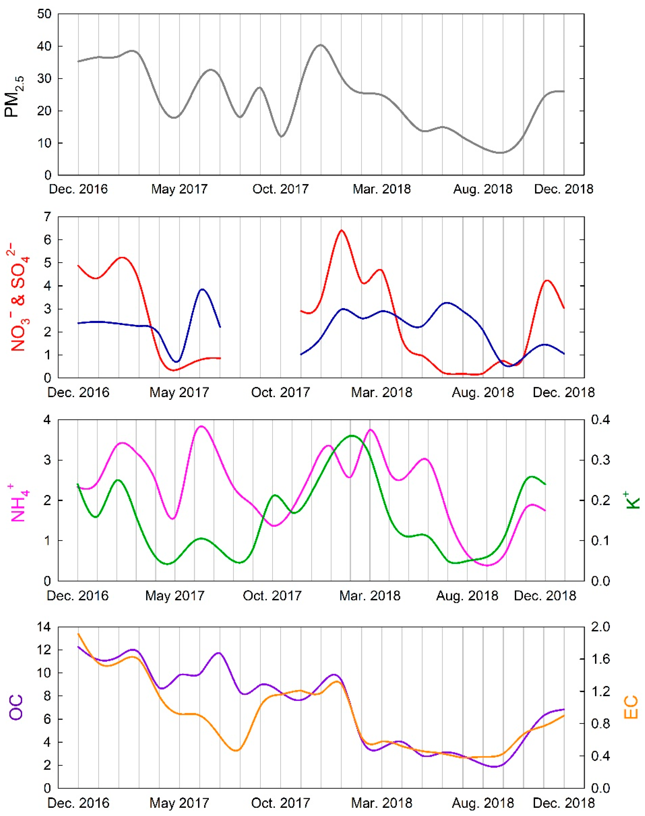
The average PM2.5 concentration was 23.2 ± 14.2 μg m−3 for the entire sampling period, which exceeds the current annual national ambient air quality standard (NAAQS) for PM2.5 (15 μg m−3). Approximately 16% of the samples (N = 31) exceeded a 24 h NAAQS (35 μg m−3), and more than 50% of the high concentration episodes were observed during winter (December, January, and February) (N = 20). There were distinct seasonal variations, with average concentrations of 23.4 ± 11.8, 16.3 ± 10.3, 18.4 ± 11.2, and 32.5 ± 16.4 μg m−3 in spring (March, April, and May), summer (June, July, and August), fall (September, October, and November), and winter, respectively (Figure 2). According to previous studies in Chuncheon [7,9,28], PM2.5 concentrations in the summer are typically much lower than in spring or winter, mainly because the prevailing westerly winds that transport material from the polluted areas of South Korea and China are dominant during the spring and winter. Relatively clean air masses are transported from the east and the south during the summer. In this study, PM2.5 was low in the summer of 2018 as anticipated; however, it was quite high in June and July of 2017, along with OC and NH4+ (Figure 2). In order to identify regional meteorological transport patterns, the backward trajectories for June and July of 2017 and 2018 were compared. Most of the backward trajectories came from Eastern China in 2017. However, in 2018, they originated from all directions, including southern and eastern areas of relatively clean air (Figure S1). In July 2017, when monthly PM2.5 concentrations were the lowest of the entire study period, the backward trajectories originated from the East and South Seas and passed through the southern and eastern regions of Korea. There is evidence that PM2.5 is typically enhanced when air masses are transported from China [31,41,42,43], which is also supported by these findings.
Among the PM2.5 constituents, OC exhibited the highest concentration (6.7 ± 4.3 μg m−3), while the EC concentration (0.9 ± 0.5 μg m−3) was quite low (Table 2). The average WSOC concentration was 4.3 ± 2.2 μg m−3, comprising a significant portion of OC. Both OC and EC exhibited their highest concentrations during the winter and their lowest concentrations during the summer, while WSOC was observed to be high during the spring (Table 2).
The average correlation coefficient (Pearson r) between OC and EC was 0.85 (Figure 3), indicating that the major sources of both carbonaceous species overlapped considerably throughout the study period. The correlation coefficient between OC and EC was higher during the spring (r = 0.91) and winter (r = 0.90), and lower during the summer (r = 0.76) and fall (r = 0.83) (Figure S2), likely because SOC was actively forming in strong solar radiation and high temperature conditions [21,44,45]. The correlations of WSOC with both OC and EC were statistically significant (Pearson r = 0.67 for OC and EC) (Figure 3). EC has been used previously as a tracer for anthropogenic combustion sources [46,47,48], while OC is either emitted by combustion and biogenic sources or formed secondarily in ambient air [49]. WSOC is also emitted by biomass burning [23,24,34,50] or is formed secondarily in ambient air [51]. The strong correlations between OC and EC and between WSOC and EC indicate that the carbonaceous compounds were likely influenced by primary combustion sources. Previous studies have suggested that the OC/EC ratio is 1.0–4.2 for a mobile source, ~7.7 for biomass burning, and 2.5–10.5 for coal combustion [52]. Based on the results of this study, which exhibited high OC/EC ratios (7.8 average) throughout the entire sampling period (7.4, 9.9, 7.2, and 7.2 for spring, summer, fall, and winter, respectively), the main combustion source was anticipated to be biomass burning. However, secondary OC was also likely important during warm months, given the highest OC/EC ratio and the lower correlation coefficient between OC and EC during the summer (Figure S2). It should be noted that OC concentrations from the initial part of the sampling period were likely overestimated (due to sorption of organic vapour) because the carbon denuder was not deployed upstream of the filter until February 2018. Subramanian et al. (2004) [53] observed an almost constant positive artefact of 0.5 μg m−3 for 24 h bare quartz samples without a denuder throughout the study period. Kim (2016) [54] and Cheng et al. (2012) [55] also showed that OC concentrations were overestimated by approximately 10% during the spring and fall and by approximately 15% during the summer, respectively, due to a positive sampling artefact.
The total contributions of the 7 ionic components (SO42-, NO3-, NH4+, Na+, K+, Mg2+, and Ca2+) to PM2.5 mass was 32.0%, and NO3- was the largest contribution to PM2.5 mass, followed by NH4+ and SO42− (Table 2). As reported by previous studies, the contribution of NO3- was high in cold months due to active gas–particle conversion at low temperatures [9,56]. However, SO42−, which is mostly formed secondarily, was the largest contributor to PM2.5 mass in the summer because of vigorous photochemical reactions that produce H2SO4, which is the intermediate species to the SO42− aerosol [57]. NH4+ did not exhibit any seasonal variations because it is mostly present as NH4NO3 and (NH4)2SO4 [58], although the average concentration was the highest during the winter (Table 2). The trends in the NO3–, SO42−, NH4+, and K+ concentrations were all very similar from November to March, indicating the effect of the same source (Figure 2).
3.2. Comparison with PM2.5 in Seoul
Since Chuncheon is −100 km east of the metropolitan area of South Korea (Seoul), its air quality is anticipated to be affected by Seoul and nearby areas via the prevailing westerly winds. In this study, we compared PM2.5 concentrations between Chuncheon and Seoul. PM2.5 concentration data from Seoul were obtained from the national ambient air quality monitoring station located at the centre of Seoul (Jung-Gu) (Figure 1). Samples from Chuncheon had PM2.5 concentrations more than 1.2 times higher than those in Seoul on day 49 during the sampling period (higher concentration in Chuncheon, HC), while samples from Chuncheon had PM2.5 concentrations more than 1.2 times lower than those in Seoul on day 106 during the sampling period (lower concentration in Chuncheon, LC). In this study, the HC sample was assumed to represent a locally occurring episode of high concentration in Chuncheon. There were 60 d with no significant difference between the two sites during the sampling period. HC samples generally were observed in 2017, while LC samples were observed in 2018 (Figure 4). It should be noted that samples were taken for 24 h until November 2017 and collected for 71 h thereafter. Therefore, the frequent occurrence of HC samples only in 2017 may suggest that high PM2.5 concentration episodes in Chuncheon were unlikely to have lasted longer than 3 d.
3.2.1. Differences between HC and LC Samples
In this study, we compared the characteristics of PM2.5 and its chemical constituents in the HC and LC samples collected at the sampling site in Chuncheon. Concentrations of most of the constituents, as well as PM2.5 mass, were higher in the HC samples than in the LC samples (Table 3). However, except for OC, the percentage of each element in the PM2.5 mass was lower in the HC samples, resulting in a higher contribution of an undetermined portion in the HC samples (Figure 5). Metallic elements that were not measured in this study are typically considered as core constituents of PM2.5. These elements are directly emitted by natural and anthropogenic sources and are not formed secondarily [59]. Therefore, a higher contribution of an undetermined PM2.5 composition indicates the potential significance of primary emission sources when PM2.5 concentrations were higher in Chuncheon than in Seoul. Excluding the undetermined fraction, the highest mass contributors were OC and EC in the HC samples, with increases of 1.8 and 1.5 times their contributions to the LC samples, respectively (Figure 5).
While PM2.5 concentrations of the HC samples were 1.7 times higher than the LC samples, the PM10 concentrations of the HC samples (43.2 ± 21.4 μg m−3) were very similar to those of the LC samples (44.5 ± 22.4 μg m−3), resulting in a much higher PM2.5/PM10 ratio for the HC samples (74.3%) than the LC samples (41.4%). Considering that the average PM2.5/PM10 ratio was 49.8% for the entire sampling period, the elevated PM2.5/PM10 ratios of the HC samples suggest that primary sources and/or secondary formation pathways that generated only PM2.5 and not PM2.5–10 caused the local high concentration episodes in Chuncheon. In addition, the correlation between PM2.5 and PM2.5–10 was statistically significant in the LC samples (r = 0.471, p < 0.001), but was not significant in the HC samples (r = 0.225, p-value = 0.193), indicating that the major sources of PM2.5 were likely different from those of PM2.5–10 when the PM2.5 concentrations in Chuncheon were higher than in Seoul.
3.2.2. Possible Sources for HC Samples
The total contributions of the seven ionic components to the PM2.5 mass were 23.1% and 40.0% for the HC and LC samples, respectively, although the PM2.5 concentrations of the HC samples were higher than those of the LC samples (Table 3). The contributions of NO3−, SO42−, and NH4+ were 6.0, 7.2, and 8.1% in the HC samples and 8.9, 13.7, and 13.6% in the LC samples, respectively. The major contribution of NH4+ among the ionic components indicates an NH4+ surplus existed when the PM2.5 concentrations were higher in Chuncheon than in Seoul. This suggests that NH3 emissions from agricultural areas, which comprise a large portion of land cover in Chuncheon, were important to increased PM2.5 concentrations. Since NH3 is not likely to undergo long-range transport due to its short atmospheric residence time [58,60], it would be useful to reduce NH3 emissions from local sources in order to reduce PM2.5 concentrations. The contribution of SO42- to the PM2.5 mass was approximately two times greater in the LC samples than the HC samples because the LC samples were often collected during warm months (the fraction of LC samples collected in spring and summer was 75% of the total samples, while the fraction of HC samples was 30%) when the formation of H2SO4 occurs due to the high concentrations of hydroxyls (OH−) [18,61].
OC and EC concentrations were higher in the HC than in the LC samples, with average values of 9.3 ± 1.1 μg m−3 and 1.1 ± 0.6 μg m−3, respectively (Table 3). The correlation coefficient between OC and EC was much higher for LC samples (r = 0.94) than for HC samples (r = 0.71) (Figure 6). In addition, the OC/EC ratios were 9.7 ± 5.2 and 7.0 ± 1.8 for the HC and LC samples, respectively. These results, including higher OC concentrations, lower correlation coefficients between OC and EC, and higher OC/EC ratios for HC samples, suggest that carbonaceous compounds were affected by diverse sources including secondary formation during high concentration episodes that occurred locally in Chuncheon. The OC/EC ratios in the HC samples during the summer were more than two times larger (16.6 ± 5.7) than those of the LC samples (7.3 ± 2.3), indicating that OC in the HC samples was mainly formed secondarily either in situ in Chuncheon, or during regional or long-range transport to Chuncheon during the summer. The secondary formation of OC is also supported by the relatively low correlation coefficients between OC and EC in the HC samples (Figure 6).
SOC was estimated indirectly using the EC tracer method [62], which assumes that primary OC can be calculated from EC concentrations using the following equation:
where b is the fraction of POC emitted along with EC from the combustion source and a indicates non-combustion-derived POC [63]. The slope, b, and the offset, a, were determined from a regression line of plotted OC vs. EC data, including points aligned at the lower end of the graph (Figure 6) [17,63,64]. The concentrations of SOC were then estimated using the following equation:
POC = b·EC + a
SOC = OC − POC = OC − (b·EC + a),
In both HC and LC samples, the fractions of POC emitted along with EC from the combustion source (slope b) were almost identical, and the non-combustion-derived POC (offset a) was negligible (Figure 6). The slope obtained in this study was somewhat larger than those obtained in previous studies (−1.0–2.5) [17,64], likely because of a smaller influence of mobile sources (with low OC/EC ratios) than other combustion sources [65] in this small city. SOC was more important in the HC samples (SOC = 4.4 ± 3.0 μg m−3, SOC/OC ratio = 47%) than in the LC samples (1.8 ± 1.7 μg m−3, 35%), which is also supported by the lower correlation coefficient between OC and EC for the HC samples than the LC samples (Figure 6). The SOC concentrations and SOC/OC fractions increased to 7.5 μg m−3 and 71% during summer in the HC samples. Relative humidity had a major impact on SOC formation [63], as aqueous phase chemistry is a major pathway for SOC formation, particularly under high NOx conditions [66,67]. Galindo et al. (2019) [63] observed significant increases in SOC concentrations when RH > 70%. In this study, the impact of RH on SOC concentration was significant only in the HC samples, and the coefficient of determination (r2) increased further when only winter data were considered (Figure 7). This result indicates that the gas–particle partitioning of organic compounds via aqueous phase reactions is important, especially during the winter, for locally occurring high concentration episodes. During other seasons, volatile organic compounds are likely converted into low-volatility products through active gas phase photochemical oxidation and condensed into the particulate phase [63,68].
Meanwhile, WSOC had a much stronger correlation with EC, as well as with OC, in the HC samples than the LC samples (Figure 6), indicating that primary combustion emissions had a significant influence on the PM2.5 carbonaceous component as a local source in Chuncheon. WSOC is known to be either directly emitted by combustion sources or formed by the oxidation of volatile organic compounds (VOCs) in the atmosphere [69]. Although secondary formation is believed to be the major formation pathway of WSOC, a number of studies have found that non-fossil fuel sources, such as biomass burning, are a major source of WSOC [70]. On the other hand, WIOC usually better represents primary OC emitted directly by fossil-fuel combustion [70]. In this study, WSOC was better correlated with EC in the HC samples than the LC samples (Figure 6), indicating that it was mainly emitted by primary combustion sources in the HC samples because EC is not a secondary pollutant [71]. WSOC was also highly correlated with secondary inorganic aerosols including NO3−, SO42−, and NH4+ as well as with K+, a marker for biomass burning, in the HC samples (Table 4), while it showed weak correlations only with OC and EC in the LC samples (Table 5). These results suggest that the strong co-emissions or common source (or formation pathway) of the highly correlated species were significant local sources in Chuncheon. It has been suggested that the particles derived from the burning of fresh biomass can be readily converted to KNO3 and K2SO4 via heterogeneous reactions [72,73]. In the HC samples, K+ was strongly correlated with NO3− (Table 4), as well as with WSOC, suggesting that biomass burning was likely an important local source for both WSOC and PM2.5 in Chuncheon.
A PCA analysis was performed for the HC samples to interpret the PM2.5 sources using PM2.5, its chemical constituents, and meteorological parameters. Four factors were extracted, which accounted for 98.5% of the total variance (Table 6). Factor 1, which contributed −63.2% of the total variance, was interpreted as fossil fuel combustion during the winter because NO2, CO, SO2, and WIOC exhibited high factor loadings, while temperature had a negative loading. Factor 2, which accounted for −20% of the total variance, exhibited high loadings of NO3−, SO42−, NH4+, K+, and WSOC, and was presumed to be biomass burning. This implies that the formation of WSOC is associated with secondary inorganic reactions in biomass burning plumes [9,72,73,74]; hence, secondary OC can also be considered to be explained by Factor 2. Factor 3 was interpreted as crustal dust, as PM2.5–10, Na+, Mg2+, and Ca2+ were all enriched. Factor 4 exhibited high loadings of temperature, RH, and NH4+, indicating secondary NH4+ formation during warm days when NH3+ emissions typically increase due to fertiliser application and cattle farming [75]. Both NO3- and SO42− did not exhibit high loadings in Factor 4, indicating that NH4+ may have existed in other forms (e.g., NH4Cl) [9] as well as (NH4)2SO4 and NH4NO3, as shown by Factor 2.
4. Conclusions
In this study, PM2.5 and its major chemical compositions were measured in Chuncheon, South Korea, a small residential city, which experiences local high PM2.5 concentration episodes that cannot be linked to particulate transport from upwind urban and industrial areas. Of the 215 samples collected in Chuncheon, 49 had PM2.5 concentrations of at least 1.2 times higher than those in the upwind metropolitan area of Seoul. While PM2.5 concentrations were clearly higher in the HC samples than in the LC samples, the PM10 concentrations were very similar to each other, suggesting that there were certain primary sources and/or secondary formations that generated only PM2.5, and not PM2.5–10. For the HC samples, PM2.5 was strongly correlated with carbonaceous compounds, including OC and EC, and the SOC fraction contributed to OC was much higher than in the LC samples, indicating the significance of the formation of secondary organic aerosols in locally occurring high PM2.5 episodes in Chuncheon. However, WSOC, a potential indicator of secondary OC or non-fossil fuel sources, was highly correlated with EC and K+ in the HC samples, suggesting that biomass burning was also an important local source in Chuncheon. A PCA analysis identified four possible factors: fossil-fuel combustion during the winter, represented by high loadings of NO2, CO, SO2, and WIOC (Factor 1); secondary inorganic and organic reactions in biomass burning plumes (Factor 2); crustal dust (Factor 3); and secondary NH4+ formation during warm days (Factor 4). Factors 2 and 4 exhibited high PM2.5 loading values, suggesting that secondary organic/inorganic formation and biomass burning were the most significant sources of variation in PM2.5 concentrations in Chuncheon. Based on the results of this study, it is clear that local policies to reduce biomass burning and NH3 emissions should be applied to decrease the PM2.5 concentrations in Chuncheon. In addition, high RH and low WS conditions in the city are suitable for the formation of secondary aerosols; therefore, cooperation with adjacent regions and countries to reduce NOx and SO2 emissions is also very important because these precursor gases can undergo long-range transport.
Supplementary Materials
The following are available online at https://www.mdpi.com/2073-4433/12/1/86/s1, Figure S1: Backward trajectories for June and July in 2017 (a) and 2018 (b); Figure S2: Relationship between OC and EC in spring (top left), summer (top right), fall (bottom left), and winter (bottom right).
Author Contributions
The work presented in this article was carried out through collaboration between all authors. S.-Y.C. analysed the data and wrote the paper. J.-Y.B. and S.-W.P. performed the experiments. Y.-J.H. acquired the funding, defined the research theme, interpreted the results, and wrote the paper. All authors have read and agreed to the published version of the manuscript.
Funding
This research was funded by a grant from the Ministry of Environment, Korea, and by a grant from the National Research Foundation of Korea (NRF-2017K1A13A1A12073373 and NRF-2020R1A2C2013445).
Institutional Review Board Statement
Not applicable.
Informed Consent Statement
Not applicable.
Data Availability Statement
Data is contained within the article.
Acknowledgments
We would like to thank the Central Laboratory of Kangwon National University for helping with chemical analysis.
Conflicts of Interest
The authors declare no conflict of interest. The funders had no role in the design of the study; in the collection, analyses, or interpretation of data; in the writing of the manuscript, or in the decision to publish the results.
References
- Jacob, D.J.; Winner, D.A. Effect of climate change on air quality. Atmos. Environ. 2009, 43, 51–63. [Google Scholar] [CrossRef] [Green Version]
- IPCC. Climate Change 2007: The Physical Science Basis. Contribution of Working Group I to the Fourth Assessment Report of the Intergovernmental Panel on Climate Change; Solomon, S., Qin, D., Manning, M., Chen, Z., Marquis, M., Averyt, K.B., Tignor, M., Miller, H.L., Eds.; Cambridge University Press: Cambridge, UK, 2007. [Google Scholar]
- Lohmann, U.; Feichter, J. Global indirect aerosol effects: A review. Atmos. Chem. Phys. Discuss. 2005, 5, 715–737. [Google Scholar] [CrossRef] [Green Version]
- Kaufman, Y.J.; Tanré, D.; Boucher, O. A satellite view of aerosols in the climate system. Nature 2002, 419, 215–223. [Google Scholar] [CrossRef] [PubMed]
- Hallquist, M.; Wenger, J.C.; Baltensperger, U.; Rudich, Y.; Simpson, D.; Claeys, M.; Dommen, J.; Donahue, N.M.; George, C.; Goldstein, A.H.; et al. The formation, properties and impact of secondary organic aerosol: Current and emerging issues. Atmos. Chem. Phys. 2009, 9, 5155–5236. [Google Scholar] [CrossRef] [Green Version]
- Choi, A.; Lee, J.; Shin, H.J.; Lee, M.; Lim, J. Characteristics of organic compounds in PM2.5 at urban and remote areas in Korea. AGUFM 2016, 2016, A51D-0077. [Google Scholar]
- Han, Y.J.; Kim, H.W.; Cho, S.H.; Kim, P.R.; Kim, W.J. Metallic elements in PM2.5 in different functional areas of Korea: Concentrations and source identifica-tion. Atmos. Res. 2015, 153, 416–428. [Google Scholar] [CrossRef]
- Byun, J.-Y.; Cho, S.-H.; Kim, H.-W.; Han, Y.-J. Long-term Characteristics of PM2.5 and Its Metallic Components in Chuncheon, Korea. J. Korean Soc. Atmos. Environ. 2018, 34, 406–417. [Google Scholar] [CrossRef]
- Byun, J.-Y.; Kim, H.; Han, Y.-J.; Lee, S.-D.; Park, S.-W. High PM2.5 Concentrations in a Small Residential City with Low Anthropogenic Emissions in South Korea. Atmosphere 2020, 11, 1159. [Google Scholar] [CrossRef]
- Xiao, R.; Takegawa, N.; Zheng, M.; Kondo, Y.; Miyazaki, Y.; Miyakawa, T.; Hu, M.; Shao, M.; Zeng, L.; Gong, Y.; et al. Characterization and source apportionment of submicron aerosol with aerosol mass spectrometer during the PRIDE-PRD 2006 campaign. Atmos. Chem. Phys. Discuss. 2011, 11, 1891–1937. [Google Scholar] [CrossRef]
- Guofeng, S.; Siye, W.; Wen, W.; Yanyan, Z.; Yujia, M.; Bin, W.; Rong, W.; Wei, L.; Huizhong, S.; Ye, H.; et al. Emission Factors, Size Distributions, and Emission Inventories of Carbonaceous Particulate Matter from Residential Wood Combustion in Rural China. Environ. Sci. Technol. 2012, 46, 4207–4214. [Google Scholar] [CrossRef] [Green Version]
- Verma, V.; Rico-Martinez, R.; Kotra, N.; King, L.; Liu, J.; Snell, T.W.; Weber, R.J. Contribution of Water-Soluble and Insoluble Components and Their Hydrophobic/Hydrophilic Subfractions to the Reactive Oxygen Species-Generating Potential of Fine Ambient Aerosols. Environ. Sci. Technol. 2012, 46, 11384–11392. [Google Scholar] [CrossRef] [PubMed]
- Timonen, H.; Carbone, S.; Aurela, M.; Saarnio, K.; Saarikoski, S.; Ng, N.L.; Canagaratna, M.R.; Kulmala, M.; Kerminen, V.-M.; Worsnop, D.R.; et al. Characteristics, sources and water-solubility of ambient submicron organic aerosol in springtime in Helsinki, Finland. J. Aerosol Sci. 2013, 56, 61–77. [Google Scholar] [CrossRef]
- Ji, D.; Yan, Y.; Wang, Z.; He, J.; Liu, B.; Sun, Y.; Gao, M.; Li, Y.; Cao, W.; Cui, Y.; et al. Two-year continuous measurements of carbonaceous aerosols in urban Beijing, China: Temporal variations, characteristics and source analyses. Chemosphere 2018, 200, 191–200. [Google Scholar] [CrossRef] [PubMed]
- Liu, H.; Tian, H.; Zhang, K.; Liu, S.; Cheng, K.; Yin, S.; Liu, Y.; Liu, X.; Wu, Y.; Liu, W.; et al. Seasonal variation, formation mechanisms and potential sources of PM2.5 in two typical cit-ies in the Central Plains Urban Agglomeration, China. Sci. Total Environ. 2019, 657, 657–670. [Google Scholar] [CrossRef]
- Liu, S.; Zhu, C.; Tian, H.; Wang, Y.; Zhang, K.; Wu, B.; Liu, X.; Hao, Y.; Liu, W.; Bai, X.; et al. Spatiotemporal Variations of Ambient Concentrations of Trace Elements in a Highly Polluted Region of China. J. Geophys. Res. Atmos. 2019, 124, 4186–4202. [Google Scholar] [CrossRef]
- Castro, L.; Pio, C.; Harrison, R.M.; Smith, D. Carbonaceous aerosol in urban and rural European atmospheres: Estimation of secondary organic carbon concentrations. Atmos. Environ. 1999, 33, 2771–2781. [Google Scholar] [CrossRef]
- Seinfeld, J.H.; Pandis, S.N.; Noone, K. Atmospheric Chemistry and Physics: From Air Pollution to Climate Change. Phys. Today 1998, 51, 88. [Google Scholar] [CrossRef]
- Weber, R.J.; Sullivan, A.P.; Peltier, R.E.; Russell, A.G.; Yan, B.; Zheng, M.; De Gouw, J.; Warneke, C.; Brock, C.; Holloway, J.S.; et al. A study of secondary organic aerosol formation in the anthropogenic-influenced southeastern United States. J. Geophys. Res. Space Phys. 2007, 112. [Google Scholar] [CrossRef]
- Park, S.; Schauer, J.J.; Cho, S.Y. Sources and their contribution to two water-soluble organic carbon fractions at a roadway site. Atmos. Environ. 2013, 77, 348–357. [Google Scholar] [CrossRef]
- Yu, G.-H.; Cho, S.-Y.; Bae, M.-S.; Park, S. Difference in production routes of water-soluble organic carbon in PM2.5 observed during non-biomass and biomass burning periods in Gwangju, Korea. Environ. Sci. Process. Impacts 2014, 16, 1726–1736. [Google Scholar] [CrossRef]
- Kuang, B.Y.; Lin, P.; Huang, X.H.H.; Yu, J.Z. Sources of humic-like substances in the Pearl River Delta, China: Positive matrix factorization analysis of PM2.5 major components and source markers. Atmos. Chem. Phys. Discuss. 2015, 15, 1995–2008. [Google Scholar] [CrossRef] [Green Version]
- Du, Z.; He, K.; Cheng, Y.; Duan, F.; Ma, Y.; Liu, J.; Zhang, X.; Zheng, M.; Weber, R. A yearlong study of water-soluble organic carbon in Beijing I: Sources and its primary vs. secondary nature. Atmos. Environ. 2014, 92, 514–521. [Google Scholar] [CrossRef]
- Wonaschutz, A.; Hersey, S.P.; Sorooshian, A.; Craven, J.S.; Metcalf, A.R.; Flagan, R.C.; Seinfeld, J.H. Impact of a large wildfire on water-soluble organic aerosol in a major urban area: The 2009 Station Fire in Los Angeles County. Atmos. Chem. Phys. Discuss. 2011, 11, 8257–8270. [Google Scholar] [CrossRef] [Green Version]
- Huang, X.F.; Yu, J.Z.; He, L.Y.; Yuan, Z. Water-soluble organic carbon and oxalate in aerosols at a coastal urban site in China: Size distribu-tion characteristics, sources, and formation mechanisms. J. Geophys. Res. Atmos. 2006, 111, D22. [Google Scholar] [CrossRef]
- Ruellan, S.; Cachier, H. Characterisation of fresh particulate vehicular exhausts near a Paris high flow road. Atmos. Environ. 2001, 35, 453–468. [Google Scholar] [CrossRef]
- Heo, J.-B.; Hopke, P.K.; Yi, S.-M. Source apportionment of PM2.5 in Seoul, Korea. Atmos. Chem. Phys. Discuss. 2009, 9, 4957–4971. [Google Scholar] [CrossRef] [Green Version]
- Cho, S.-H.; Kim, P.-R.; Han, Y.-J.; Kim, H.-W.; Yi, S.-M. Characteristics of Ionic and Carbonaceous Compounds in PM2.5 and High Concentration Events in Chuncheon, Korea. J. Korean Soc. Atmos. Environ. 2016, 32, 435–447. [Google Scholar] [CrossRef] [Green Version]
- IQAir AirVisual. 2018 World Air Quality Report; Region & City PM2.5 Ranking; IQAir AirVisual: 2018. Available online: https://www.iqair.com/world-most-polluted-cities/world-air-quality-report-2018-en.pdf (accessed on 6 January 2021).
- Jung, J.-H.; Han, Y.-J. Study on Characteristics of PM2.5 and Its Ionic Constituents in Chuncheon, Korea. J. Korean Soc. Atmos. Environ. 2008, 24, 682–692. [Google Scholar] [CrossRef] [Green Version]
- Han, Y.-J.; Kim, T.-S.; Kim, H. Ionic constituents and source analysis of PM2.5 in three Korean cities. Atmos. Environ. 2008, 42, 4735–4746. [Google Scholar] [CrossRef]
- Vellingiri, K.; Kim, K.-H.; Ma, C.-J.; Kang, C.-H.; Lee, J.-H.; Kim, I.-S.; Brown, R.J. Ambient particulate matter in a central urban area of Seoul, Korea. Chemosphere 2015, 119, 812–819. [Google Scholar] [CrossRef]
- Bari, A.; Kindzierski, W.B. Concentrations, sources and human health risk of inhalation exposure to air toxics in Edmonton, Canada. Chemosphere 2017, 173, 160–171. [Google Scholar] [CrossRef]
- Tian, Y.; Chen, J.-B.; Zhang, L.-L.; Du, X.; Wei, J.-J.; Fan, H.; Xu, J.; Wang, H.-T.; Guan, L.; Shi, G.-L.; et al. Source profiles and contributions of biofuel combustion for PM2.5, PM10 and their compositions, in a city influenced by biofuel stoves. Chemosphere 2017, 189, 255–264. [Google Scholar] [CrossRef]
- Kang, C.-M.; Kang, B.-W.; Lee, H.S. Source identification and trends in concentrations of gaseous and fine particulate principal species in Seoul, South Korea. J. Air Waste Manag. Assoc. 2006, 56, 911–921. [Google Scholar] [CrossRef] [Green Version]
- Khare, P.; Baruah, B.P. Elemental characterization and source identification of PM2. 5 using multivariate anal-ysis at the suburban site of North-East India. Atmos. Res. 2010, 98, 148–162. [Google Scholar] [CrossRef]
- Song, Y.; Zhang, Y.; Xie, S.; Zeng, L.; Zheng, M.; Salmon, L.G.; Shao, M.; Slanina, S. Source apportionment of PM2.5 in Beijing by positive matrix factorization. Atmos. Environ. 2006, 40, 1526–1537. [Google Scholar] [CrossRef]
- Paatero, P.; Tapper, U. Positive matrix factorization: A non-negative factor model with optimal utilization of error estimates of data values. Environmetrics 1994, 5, 111–126. [Google Scholar] [CrossRef]
- Birch, M.E.; Cary, R.A. Elemental Carbon-Based Method for Monitoring Occupational Exposures to Particulate Diesel Exhaust. Aerosol Sci. Technol. 1996, 25, 221–241. [Google Scholar] [CrossRef]
- Park, S.; Bae, M.S.; Schauer, J.J.; Ryu, S.Y.; Kim, Y.J.; Cho, S.Y.; Kim, S.J. Evaluation of the TMO and TOT methods for OC and EC measurements and their characteristics in PM2.5 at an urban site of Korea during ACE-Asia. Atmos. Environ. 2005, 39, 5101–5112. [Google Scholar] [CrossRef]
- Sahu, L.K.; Kondo, Y.; Miyazaki, Y.; Kuwata, M.; Koike, M.; Takegawa, N.; Tanimoto, H.; Matsueda, H.; Yoon, S.C.; Kim, Y.J. Anthropogenic aerosols observed in Asian continental outflow at Jeju Island, Korea, in spring 2005. J. Geophys. Res. Space Phys. 2009, 114, D3. [Google Scholar] [CrossRef]
- Pani, S.K.; Ou-Yang, C.-F.; Wang, S.-H.; Ogren, J.A.; Sheridan, P.J.; Sheu, G.-R.; Lin, N.-H. Relationship between long-range transported atmospheric black carbon and carbon monoxide at a high-altitude background station in East Asia. Atmos. Environ. 2019, 210, 86–99. [Google Scholar] [CrossRef]
- Kanaya, Y.; Pan, X.; Miyakawa, T.; Komazaki, Y.; Taketani, F.; Uno, I.; Kondo, Y. Long-term observations of black carbon mass concentrations at Fukue Island, western Japan, during 2009–2015: Constraining wet removal rates and emission strengths from East Asia. Atmos. Chem. Phys. Discuss. 2016, 16, 10689–10705. [Google Scholar] [CrossRef] [Green Version]
- Sullivan, A.P.; Weber, R.J. Chemical characterization of the ambient organic aerosol soluble in water: 1. Isolation of hydrophobic and hydrophilic fractions with a XAD-8 resin. J. Geophys. Res. Space Phys. 2006, 111, 111. [Google Scholar] [CrossRef] [Green Version]
- Jung, J.; Kim, Y.J. Tracking sources of severe haze episodes and their physicochemical and hygroscopic properties under Asian continental outflow: Long-range transport pollution, postharvest biomass burning, and Asian dust. J. Geophys. Res. Space Phys. 2011, 116, 116. [Google Scholar] [CrossRef]
- Lee, H.-W.; Lee, T.-J.; Kim, D.-S. Identifying Ambient PM2.5 Sources and Estimating their Contributions by Using PMF: Separation of Gasoline and Diesel Automobile Sources by Analyzing ECs and OCs. J. Korean Soc. Atmos. Environ. 2009, 25, 75–89. [Google Scholar] [CrossRef] [Green Version]
- Ho, K.; Lee, S.; Chan, C.K.; Yu, J.C.; Chow, J.C.; Yao, X. Characterization of chemical species in PM2.5 and PM10 aerosols in Hong Kong. Atmos. Environ. 2003, 37, 31–39. [Google Scholar] [CrossRef]
- Streets, D.G.; Bond, T.C.; Carmichael, G.R.; Fernandes, S.D.; Fu, Q.; He, D.; Klimont, Z.; Nelson, S.M.; Tsai, N.Y.; Wang, M.Q.; et al. An inventory of gaseous and primary aerosol emissions in Asia in the year 2000. J. Geophys. Res. Space Phys. 2003, 108, GTE-30. [Google Scholar] [CrossRef]
- Park, S.; Hur, J.-Y.; Cho, S.-Y.; Kim, S.-J.; Kim, Y.-J. Characteristics of Organic Carbon Species in Atmospheric Aerosol Particles at a Gwangju Area During Summer and Winter. J. Korean Soc. Atmos. Environ. 2007, 23, 675–688. [Google Scholar] [CrossRef] [Green Version]
- Park, S.; Cho, S.Y. Tracking sources and behaviors of water-soluble organic carbon in fine particulate matter measured at an urban site in Korea. Atmos. Environ. 2011, 45, 60–72. [Google Scholar] [CrossRef]
- Kawamura, K.; Seméré, R.; Imai, Y.; Fujii, Y.; Hayashi, M. Water soluble dicarboxylic acids and related compounds in Antarctic aerosols. J. Geophys. Res. Space Phys. 1996, 101, 18721–18728. [Google Scholar] [CrossRef]
- Schauer, J.J.; Kleeman, M.J.; Cass, G.R.; Simoneit, B.R. Measurement of emissions from air pollution sources. 5. C1− C32 organic compounds from gaso-line-powered motor vehicles. Environ. Sci. Technol. 2002, 36, 1169–1180. [Google Scholar] [CrossRef]
- Subramanian, R.; Khlystov, A.Y.; Cabada, J.C.; Robinson, A.L. Positive and negative artifacts in particulate organic carbon measurements with denuded and un-denuded sampler configurations special issue of aerosol science and technology on findings from the fine particulate matter supersites program. Aerosol Sci. Technol. 2004, 38, 27–48. [Google Scholar] [CrossRef] [Green Version]
- Kim, D.-Y. The Effect of Gas Phase Organic Carbon for the Determination of Particulate Organic Carbon and Elemental Carbon in the Atmosphere. Master’s Thesis, Hannam University, Chungcheong, Korea, 2016. [Google Scholar]
- Cheng, Y.; Duan, F.K.; He, K.B.; Du, Z.Y.; Zheng, M.; Ma, Y.L. Sampling artifacts of organic and inorganic aerosol: Implications for the speciation measurement of par-ticulate matter. Atmos. Environ. 2012, 55, 229–233. [Google Scholar] [CrossRef]
- Finlayson–Pitts, B.J.; Pitts, J.N.J. Chemistry of the Upper and Lower Atmosphere; Academic Press: San Diego, CA, USA, 2000; pp. 349–360. [Google Scholar]
- Christoforou, C.S.; Salmon, L.G.; Hannigan, M.P.; Solomon, P.A.; Cass, G.R. Trends in fine particle concentration and chemical composition in southern California. J. Air Waste Manag. Assoc. 2000, 50, 43–53. [Google Scholar] [CrossRef] [Green Version]
- Won, S.-R.; Choi, Y.-J.; Kim, A.-R.; Choi, S.-H.; Kim, Y.-S.; Kang, C.-H. Ionic Compositions of Particulate Matter in Yong-in in Spring and November. In: Proceedings of the Ko-rea Air Pollution Research Association Conference. Korean Soc. Atmos. Environ. 2008, 24, 175–176. [Google Scholar]
- Pekney, N.J.; Davidson, C.I.; Zhou, L.; Hopke, P.K. Application of PSCF and CPF to PMF-Modeled Sources of PM2.5 in Pittsburgh. Aerosol Sci. Technol. 2006, 40, 952–961. [Google Scholar] [CrossRef] [Green Version]
- Kim, Y.-P. Air pollution in Seoul caused by aerosols. J. Korean Soc. Atmos. Environ. 2006, 22, 535–553. [Google Scholar]
- Eatough, D.J.; Caka, F.M.; Farber, R.J. The conversion of SO2 to suflate in the atmosphere. Israel J. Chem. 1994, 34, 301–314. [Google Scholar]
- Turpin, B.J.; Huntzicker, J.J. Identification of secondary organic aerosol episodes and quantitation of primary and secondary organic aerosol concentrations during SCAQS. Atmos. Environ. 1995, 29, 3527–3544. [Google Scholar] [CrossRef]
- Galindo, N.; Yubero, E.; Clemente, A.; Nicolás, J.; Navarro-Selma, B.; Crespo, J. Insights into the origin and evolution of carbonaceous aerosols in a mediterranean urban environment. Chemosphere 2019, 235, 636–642. [Google Scholar] [CrossRef]
- Yubero, E.; Galindo, N.; Nicolas, J.-F.; Crespo, J.; Calzolai, G.; Lucarelli, F. Temporal variations of PM1 major components in an urban street canyon. Environ. Sci. Pollut. Res. 2015, 22, 13328–13335. [Google Scholar] [CrossRef]
- Lee, Y.-J.; Park, M.-K.; Jung, S.-A.; Kim, S.-J.; Jo, M.-R.; Song, I.-H.; Lyu, Y.-S.; Lim, Y.-J.; Kim, J.-H.; Jung, H.-J.; et al. Characteristics of Particulate Carbon in the Ambient Air in the Korean Peninsula. J. Korean Soc. Atmos. Environ. 2015, 31, 330–344. [Google Scholar] [CrossRef]
- Ervens, B.; Turpin, B.J.; Weber, R.J. Secondary organic aerosol formation in cloud droplets and aqueous particles (aqSOA): A review of laboratory, field and model studies. Atmos. Chem. Phys. Discuss. 2011, 11, 22301–22383. [Google Scholar] [CrossRef]
- Liu, J.-M.; Du, Z.-Y.; Gordon, M.; Liang, L.; Ma, Y.; Zheng, M.; Cheng, Y.; He, K.-B. The characteristics of carbonaceous aerosol in Beijing during a season of transition. Chemosphere 2018, 212, 1010–1019. [Google Scholar] [CrossRef] [PubMed]
- Kroll, J.H.; Seinfeld, J.H. Chemistry of secondary organic aerosol: Formation and evolution of low-volatility organics in the atmosphere. Atmos. Environ. 2008, 42, 3593–3624. [Google Scholar] [CrossRef]
- Kumagai, K.; Iijima, A.; Tago, H.; Tomioka, A.; Kozawa, K.; Sakamoto, K. Seasonal characteristics of water-soluble organic carbon in atmospheric particles in the inland Kanto plain, Japan. Atmos. Environ. 2009, 43, 3345–3351. [Google Scholar] [CrossRef]
- Zhang, Y.-L.; Li, J.; Zhang, G.; Zotter, P.; Huang, R.-J.; Tang, J.-H.; Wacker, L.; Prévôt, A.S.H.; Szidat, S. Radiocarbon-Based Source Apportionment of Carbonaceous Aerosols at a Regional Background Site on Hainan Island, South China. Environ. Sci. Technol. 2014, 48, 2651–2659. [Google Scholar] [CrossRef] [PubMed]
- Kim, H.; Jung, J.; Lee, J.; Lee, S. Seasonal characteristics of organic carbon and elemental carbon in PM2.5 in Daejeon. J. Korean Soc. Atmos. Environ. 2015, 31, 28–40. [Google Scholar] [CrossRef] [Green Version]
- Li, J.; Pósfai, M.; Hobbs, P.V.; Buseck, P.R. Individual aerosol particles from biomass burning in southern Africa: 2, Compositions and aging of inorganic particles. J. Geophys. Res. Space Phys. 2003, 108, 8484. [Google Scholar] [CrossRef] [Green Version]
- Liu, X.D.; Van Espen, P.; Adams, F.; Cafmeyer, J.; Maenhaut, W. Biomass burning in southern Africa: Individual particle characterization of atmospheric aerosols and savanna fir samples. J. Atmos. Chem. 2000, 36, 135–155. [Google Scholar] [CrossRef]
- Wen, J.; Shi, G.; Tian, Y.; Chen, G.; Liu, J.; Huang-Fu, Y.; Ivey, C.E.; Feng, Y. Source contributions to water-soluble organic carbon and water-insoluble organic carbon in PM2.5 during Spring Festival, heating and non-heating seasons. Ecotoxicol. Environ. Saf. 2018, 164, 172–180. [Google Scholar] [CrossRef]
- Park, J.; Ryoo, J.; Lee, J.; Song, M. Origins and distributions of atmospheric ammonia in Jeonju during 2019–2020. J. Korean Soc. Atmos. Environ. 2020, 36, 262–274. [Google Scholar] [CrossRef]
Figure 1.
Sampling site used in this study. Location of South Korea (left). Map of South Korea (right). Red star indicates the location of the PM2.5 sampling site in Chuncheon, and the blue circle indicates the national ambient air quality monitoring station in Seoul.
Figure 1.
Sampling site used in this study. Location of South Korea (left). Map of South Korea (right). Red star indicates the location of the PM2.5 sampling site in Chuncheon, and the blue circle indicates the national ambient air quality monitoring station in Seoul.

Figure 2.
Monthly concentrations of PM2.5 and its major components expressed as arithmetic means. Units are μg m−3 for PM2.5 and its species.
Figure 2.
Monthly concentrations of PM2.5 and its major components expressed as arithmetic means. Units are μg m−3 for PM2.5 and its species.

Figure 3.
Correlations between EC and OC (left) and between WSOC and EC (green squares) and between WSOC and OC (orange circles).
Figure 3.
Correlations between EC and OC (left) and between WSOC and EC (green squares) and between WSOC and OC (orange circles).

Figure 4.
Monthly occurrence rates of higher concentration (HC) and lower concentration (LC) samples throughout the sampling period.
Figure 4.
Monthly occurrence rates of higher concentration (HC) and lower concentration (LC) samples throughout the sampling period.

Figure 5.
Concentrations of PM2.5 components (left) and the fraction of each component in the PM2.5 mass (right) for HC and LC samples. Green circles in the left plot indicate the concentration ratios of HC to LC samples for each PM2.5 component.
Figure 5.
Concentrations of PM2.5 components (left) and the fraction of each component in the PM2.5 mass (right) for HC and LC samples. Green circles in the left plot indicate the concentration ratios of HC to LC samples for each PM2.5 component.

Figure 6.
Correlations between carbonaceous compounds in the HC (left panels) and LC (right panels) samples.
Figure 6.
Correlations between carbonaceous compounds in the HC (left panels) and LC (right panels) samples.

Figure 7.
The effect of RH on SOC concentrations for all HC samples (left) and only winter HC samples (right).
Figure 7.
The effect of RH on SOC concentrations for all HC samples (left) and only winter HC samples (right).


Table 1.
Summarized QA/QC results for PM2.5 components.
| NO3− | SO42− | Na+ | NH4+ | K+ | Mg2+ | Ca2+ | OC | EC | WSOC | |
|---|---|---|---|---|---|---|---|---|---|---|
| F.B. (μg m−3) | 0.11 | 0.15 | 0.05 | 1.08 | 0.02 | 0.002 | 0.05 | 0.36 | 0.001 | 1.83 |
| MDL (μg m−3) | 0.20 | 0.23 | 0.07 | 0.81 | 0.05 | 0.003 | 0.04 | 0.42 | 0.093 | 1.42 |
| <MDL * (%) | 21.1 | 6.2 | 21.4 | 14.8 | 16.8 | 12.2 | 13.8 | 0.5 | 0.5 | 7.3 |
| RPD (%) | 2.37 | 1.67 | 0.47 | 0.38 | 0.30 | 0.18 | 0.19 | 5.11 | 6.46 | 1.28 |
* indicates the percentage of samples below the method detection limit (MDL).
Table 2.
Seasonally averaged PM2.5 constituent concentrations (μg m−3).
| Spring | Summer | Fall | Winter | Annual | |
|---|---|---|---|---|---|
| OC | 6.3 ± 4.3 | 5.1 ± 4.0 | 6.0 ± 3.4 | 8.9 ± 4.5 | 6.7 ± 4.3 |
| EC | 0.8 ± 0.5 | 0.5 ± 0.3 | 0.8 ± 0.5 | 1.2 ± 0.6 | 0.9 ± 0.5 |
| WSOC | 5.1 ± 2.5 | 3.2 ± 2.0 | 4.5 ± 1.9 | 4.3 ± 2.2 | |
| SO42− | 2.2 ± 1.6 | 2.8 ± 1.8 | 0.9 ± 0.8 | 2.2 ± 1.7 | 2.1 ± 1.7 |
| NO3− | 2.1 ± 2.3 | 0.4 ± 0.6 | 1.7 ± 2.2 | 4.5 ± 3.4 | 2.4 ± 3.0 |
| NH4+ | 2.8 ± 1.5 | 2.2 ± 1.5 | 1.2 ± 1.0 | 2.6 ± 1.5 | 2.3 ± 1.5 |
| Na+ | 0.23 ± 0.33 | 0.17 ± 0.13 | 0.14 ± 0.18 | 0.29 ± 0.43 | 0.22 ± 0.31 |
| K+ | 0.16 ± 0.14 | 0.07 ± 0.01 | 0.14 ± 0.10 | 0.26 ± 0.15 | 0.16 ± 0.14 |
| Mg2+ | 0.06 ± 0.06 | 0.01 ± 0.01 | 0.02 ± 0.01 | 0.05 ± 0.05 | 0.01 ± 0.05 |
| Ca2+ | 0.18 ± 0.23 | 0.04 ± 0.02 | 0.28 ± 0.68 | 0.15 ± 0.13 | 0.16 ± 0.36 |
Table 3.
Average PM2.5 concentrations of HC, LC, and other samples and their major chemical components.
Table 3.
Average PM2.5 concentrations of HC, LC, and other samples and their major chemical components.
| Type | PM2.5 | PM10 | NO3− | SO42− | Na+ | NH4+ | K+ | Mg2+ | Ca2+ | OC | EC | WSOC |
|---|---|---|---|---|---|---|---|---|---|---|---|---|
| HC | 32.1 ± 15.9 | 43.2 ± 21.4 | 2.5 ± 3.2 | 2.3 ± 1.6 | 0.24 ± 0.35 | 2.5 ± 1.4 | 0.17 ± 0.12 | 0.03 ± 0.05 | 0.13 ± 0.12 | 9.3 ± 4.3 | 1.1 ± 0.6 | 4.0 ± 2.1 |
| LC | 18.4 ± 11.7 | 44.5 ± 22.4 | 1.9 ± 2.3 | 2.0 ± 1.5 | 0.19 ± 0.20 | 2.2 ± 1.6 | 0.15 ± 0.15 | 0.03 ± 0.05 | 0.15 ± 0.31 | 5.2 ± 3.6 | 0.7 ± 0.5 | 4.8 ± 2.2 |
Table 4.
Pearson correlation coefficients between PM2.5 components in HC samples. Number in bold with two starts and with one star indicate that the correlations were significant at the 0.01 and 0.05 levels, respectively.
Table 4.
Pearson correlation coefficients between PM2.5 components in HC samples. Number in bold with two starts and with one star indicate that the correlations were significant at the 0.01 and 0.05 levels, respectively.
| NO3 | SO4 | Na | NH4 | K | Mg | Ca | OC | EC | WSOC | |
|---|---|---|---|---|---|---|---|---|---|---|
| PM2.5 | 0.71 ** | 0.32 | 0.44 ** | 0.64 ** | 0.64 ** | 0.53 ** | 0.16 | 0.83 ** | 0.79 ** | 0.86 ** |
| NO3 | 1 | |||||||||
| SO4 | 0.28 | 1 | ||||||||
| Na | 0.37 | 0.20 | 1 | |||||||
| NH4 | 0.53 * | 0.70 ** | 0.42 ** | 1 | ||||||
| K | 0.94 ** | 0.24 | 0.20 | 0.41 ** | 1 | |||||
| Mg | 0.46 | −0.17 | 0.76 ** | 0.36 * | 0.29 | 1 | ||||
| Ca | 0.18 | −0.29 | 0.55 ** | 0.04 | 0.25 | 0.59 ** | 1 | |||
| OC | 0.72 ** | 0.34 | 0.44 ** | 0.42 * | 0.50 ** | 0.37 * | −0.02 | 1 | ||
| EC | 0.72 ** | 0.08 | 0.32 | 0.27 | 0.60 ** | 0.55 ** | 0.10 | 0.71 ** | 1 | |
| WSOC | 0.91 * | 0.86 * | 0.45 * | 0.71 ** | 0.76 ** | 0.56 ** | 0.21 | 0.83 ** | 0.83 ** | 1 |
Table 5.
Pearson correlation coefficients between PM2.5 components in LC samples. Number in bold with two starts and with one star indicate that the correlations were significant at the 0.01 and 0.05 levels, respectively.
Table 5.
Pearson correlation coefficients between PM2.5 components in LC samples. Number in bold with two starts and with one star indicate that the correlations were significant at the 0.01 and 0.05 levels, respectively.
| NO3 | SO4 | Na | NH4 | K | Mg | Ca | OC | EC | WSOC | |
|---|---|---|---|---|---|---|---|---|---|---|
| PM2.5 | 0.70 ** | 0.53 ** | 0.12 | 0.72 ** | 0.67 ** | 0.37 ** | 0.09 | 0.69 ** | 0.67 ** | 0.23 |
| NO3 | 1 | |||||||||
| SO4 | 0.33 * | 1 | ||||||||
| Na | 0.18 | 0.14 | 1 | |||||||
| NH4 | 0.54 ** | 0.60 ** | 0.09 | 1 | ||||||
| K | 0.76 ** | 0.40 ** | 0.05 | 0.66 ** | 1 | |||||
| Mg | 0.24 | 0.10 | 0.33 ** | 0.16 | 0.01 | 1 | ||||
| Ca | 0.21 | −0.06 | 0.39 ** | −0.01 | 0.10 | 0.26 * | 1 | |||
| OC | 0.52 ** | 0.21 | 0.27 * | 0.39 ** | 0.40 ** | 0.47 ** | 0.10 | 1 | ||
| EC | 0.54 ** | 0.19 | 0.26 * | 0.38 ** | 0.44 ** | 0.46 ** | 0.08 | 0.94 ** | 1 | |
| WSOC | −0.40 | −0.04 | −0.02 | 0.04 | −0.15 | 0.44 * | 0.19 | 0.43 * | 0.39 * | 1 |
Table 6.
Factor loadings in PM2.5 components with representative gaseous pollutants and meteorological parameters from principal component analysis (PCA).
Table 6.
Factor loadings in PM2.5 components with representative gaseous pollutants and meteorological parameters from principal component analysis (PCA).
| Factor 1 | Factor 2 | Factor 3 | Factor 4 | |
|---|---|---|---|---|
| PM2.5 | 0.478 | 0.602 | 0.185 | 0.591 |
| PM2.5−10 | 0.206 | 0.190 | 0.919 | 0.190 |
| O3 | −0.870 | −0.301 | 0.016 | 0.381 |
| NO2 | 0.886 | 0.444 | −0.025 | 0.129 |
| CO | 0.859 | 0.489 | −0.120 | 0.026 |
| SO2 | 0.845 | 0.428 | −0.069 | 0.174 |
| T | 0.044 | 0.101 | 0.504 | 0.842 |
| RH | 0.641 | 0.516 | 0.088 | 0.557 |
| WS | −0.871 | −0.038 | −0.161 | −0.448 |
| NO3− | 0.391 | 0.911 | 0.018 | 0.089 |
| SO42− | 0.205 | 0.962 | 0.148 | −0.006 |
| Na+ | −0.008 | 0.271 | 0.958 | 0.049 |
| NH4+ | 0.253 | 0.726 | 0.166 | 0.612 |
| K+ | 0.398 | 0.915 | 0.062 | 0.016 |
| Mg2+ | 0.378 | −0.110 | 0.841 | 0.353 |
| Ca2+ | −0.469 | 0.020 | 0.878 | 0.048 |
| OC | 0.637 | 0.666 | 0.256 | 0.270 |
| EC | 0.874 | 0.382 | 0.137 | 0.258 |
| WSOC | 0.445 | 0.789 | 0.213 | 0.321 |
| WIOC | 0.758 | 0.544 | 0.279 | 0.220 |
| Variance explained (%) | 63.2 | 83.0 | 92.2 | 98.5 |
Publisher’s Note: MDPI stays neutral with regard to jurisdictional claims in published maps and institutional affiliations. |
© 2021 by the authors. Licensee MDPI, Basel, Switzerland. This article is an open access article distributed under the terms and conditions of the Creative Commons Attribution (CC BY) license (http://creativecommons.org/licenses/by/4.0/).
Share and Cite
MDPI and ACS Style
Choi, S.-Y.; Park, S.-W.; Byun, J.-Y.; Han, Y.-J. Characteristics of Locally Occurring High PM2.5 Concentration Episodes in a Small City in South Korea. Atmosphere 2021, 12, 86. https://doi.org/10.3390/atmos12010086
AMA Style
Choi S-Y, Park S-W, Byun J-Y, Han Y-J. Characteristics of Locally Occurring High PM2.5 Concentration Episodes in a Small City in South Korea. Atmosphere. 2021; 12(1):86. https://doi.org/10.3390/atmos12010086
Chicago/Turabian StyleChoi, Su-Yeon, Sung-Won Park, Jin-Yeo Byun, and Young-Ji Han. 2021. "Characteristics of Locally Occurring High PM2.5 Concentration Episodes in a Small City in South Korea" Atmosphere 12, no. 1: 86. https://doi.org/10.3390/atmos12010086
Note that from the first issue of 2016, this journal uses article numbers instead of page numbers. See further details here.