ROMS Based Hydrodynamic Modelling Focusing on the Belgian Part of the Southern North Sea

 , , , , ,
Abstract
:1. Introduction
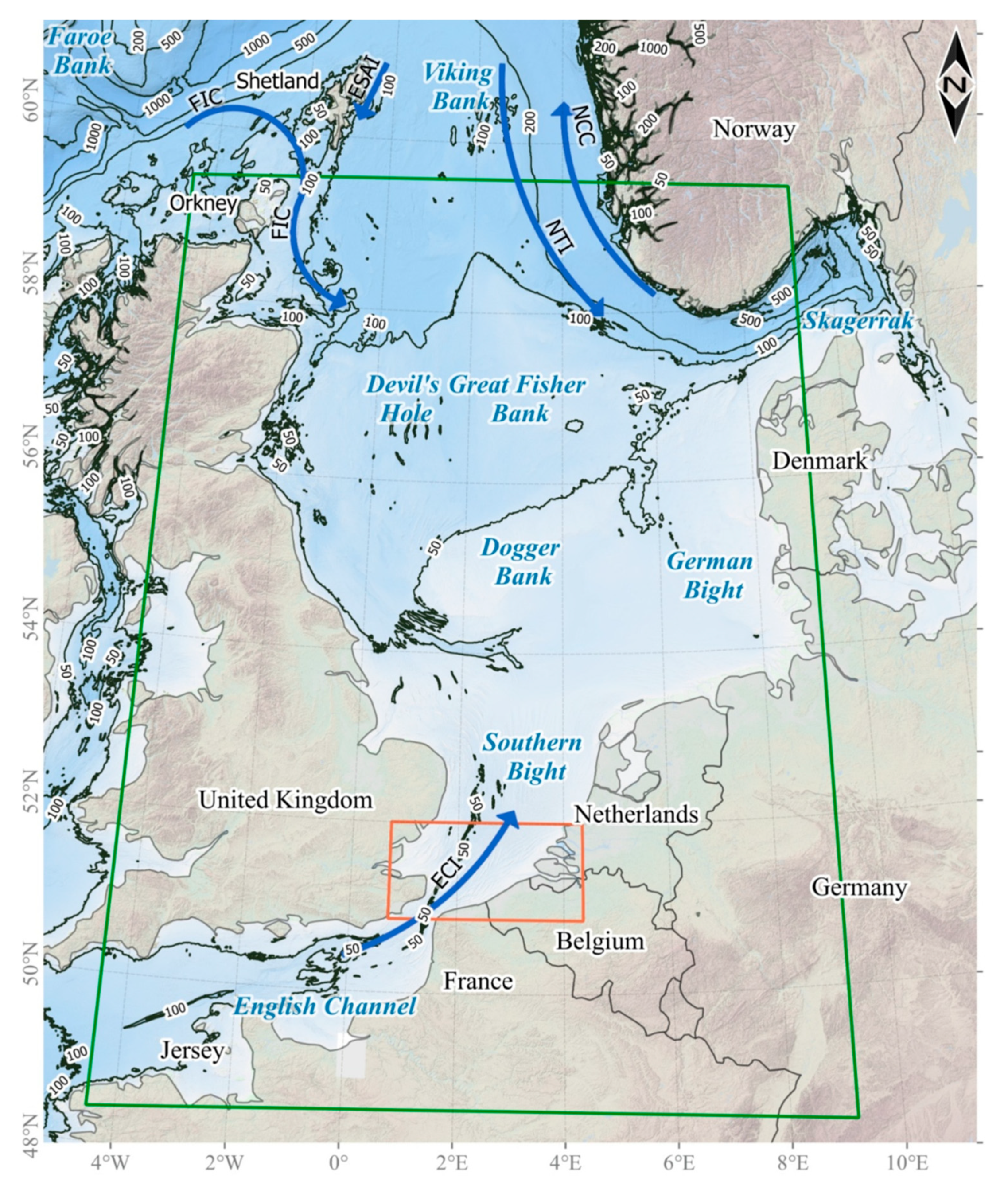
2. Dynamics of the North Sea
3. Model Configuration
3.1. Mathematical Background
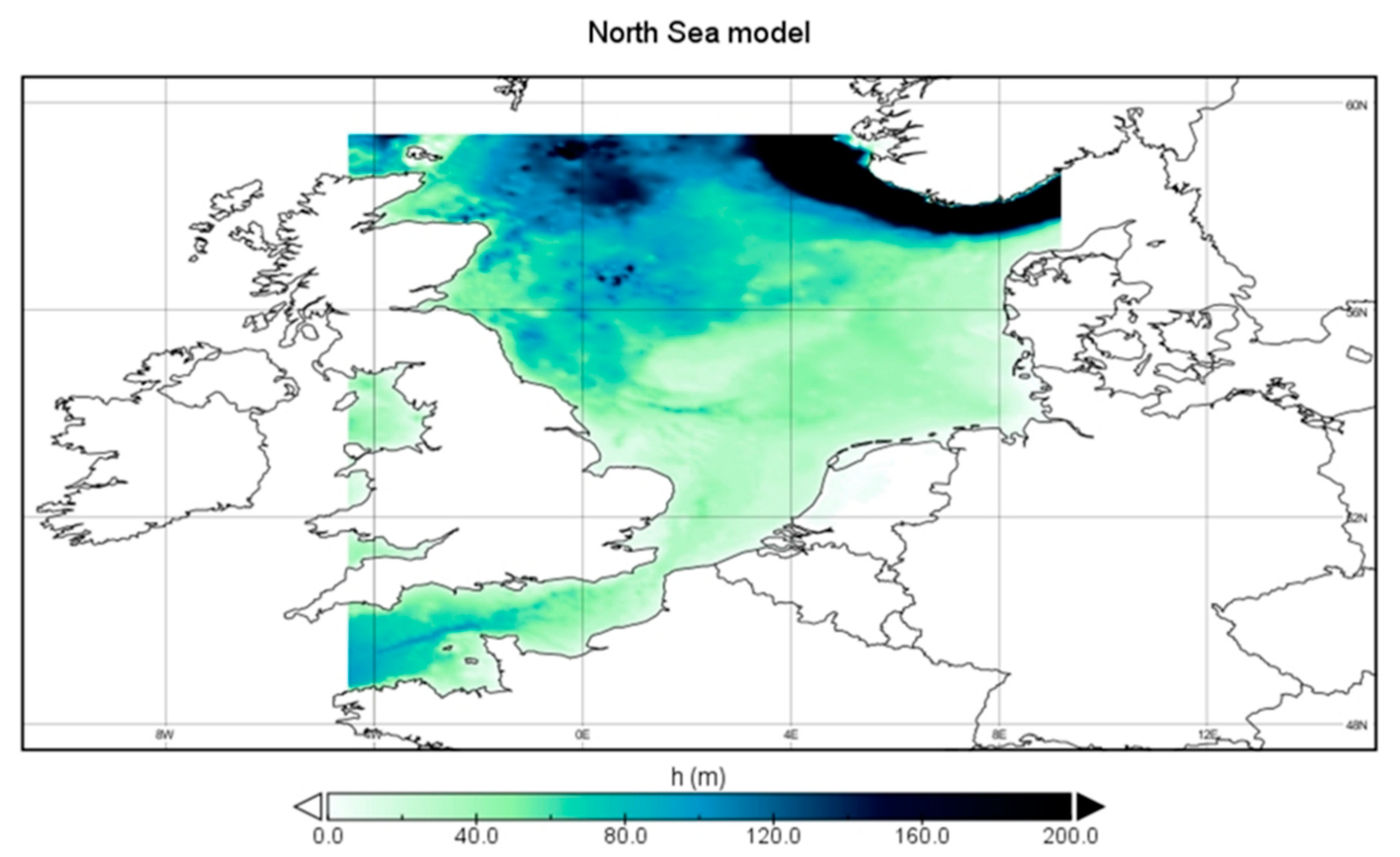
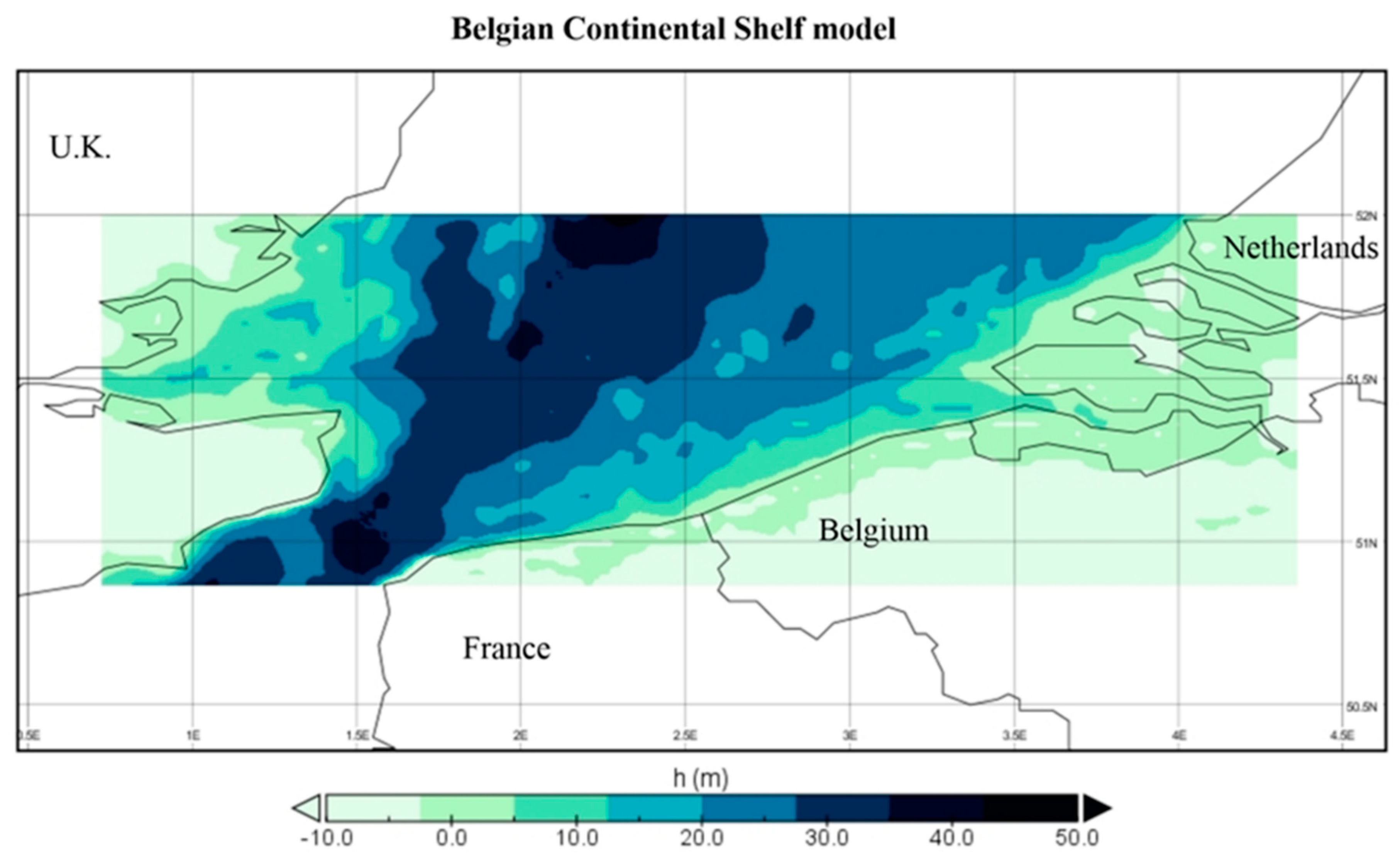
3.2. Study Area—Computational Grid
3.3. Model Settings
3.4. Model Forcing
4. Model Validation
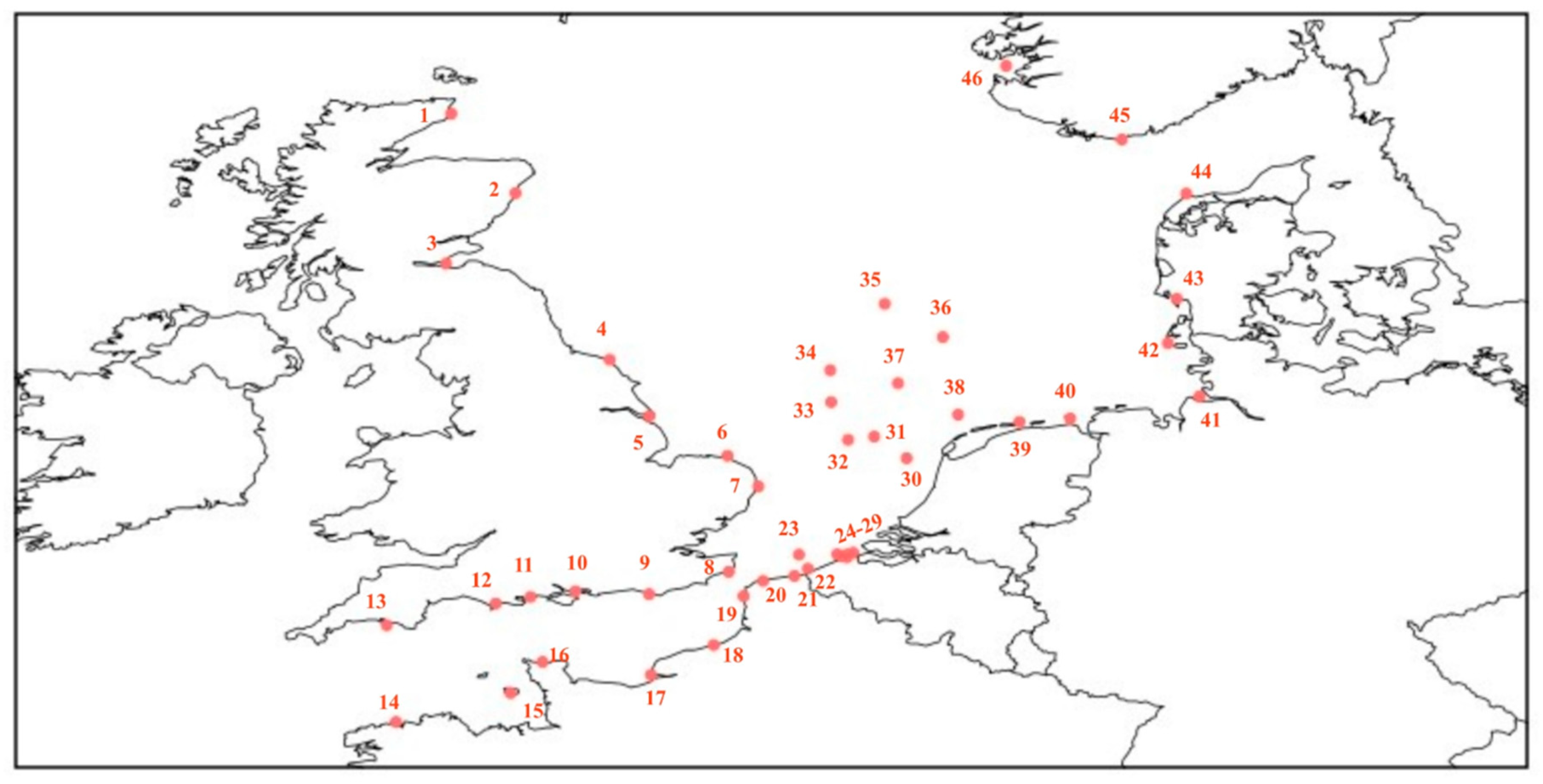
4.1. Observational Data
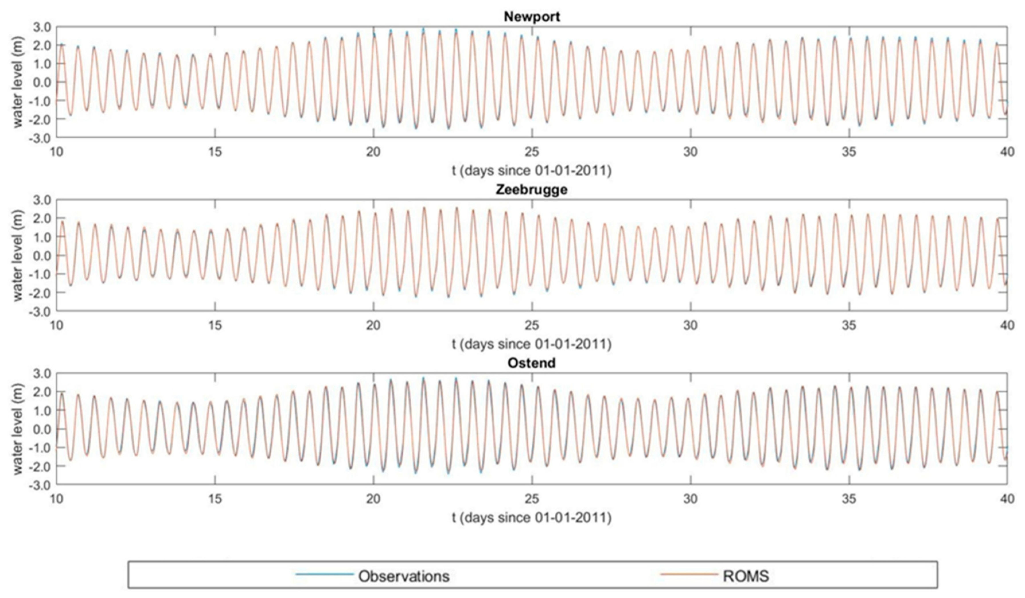
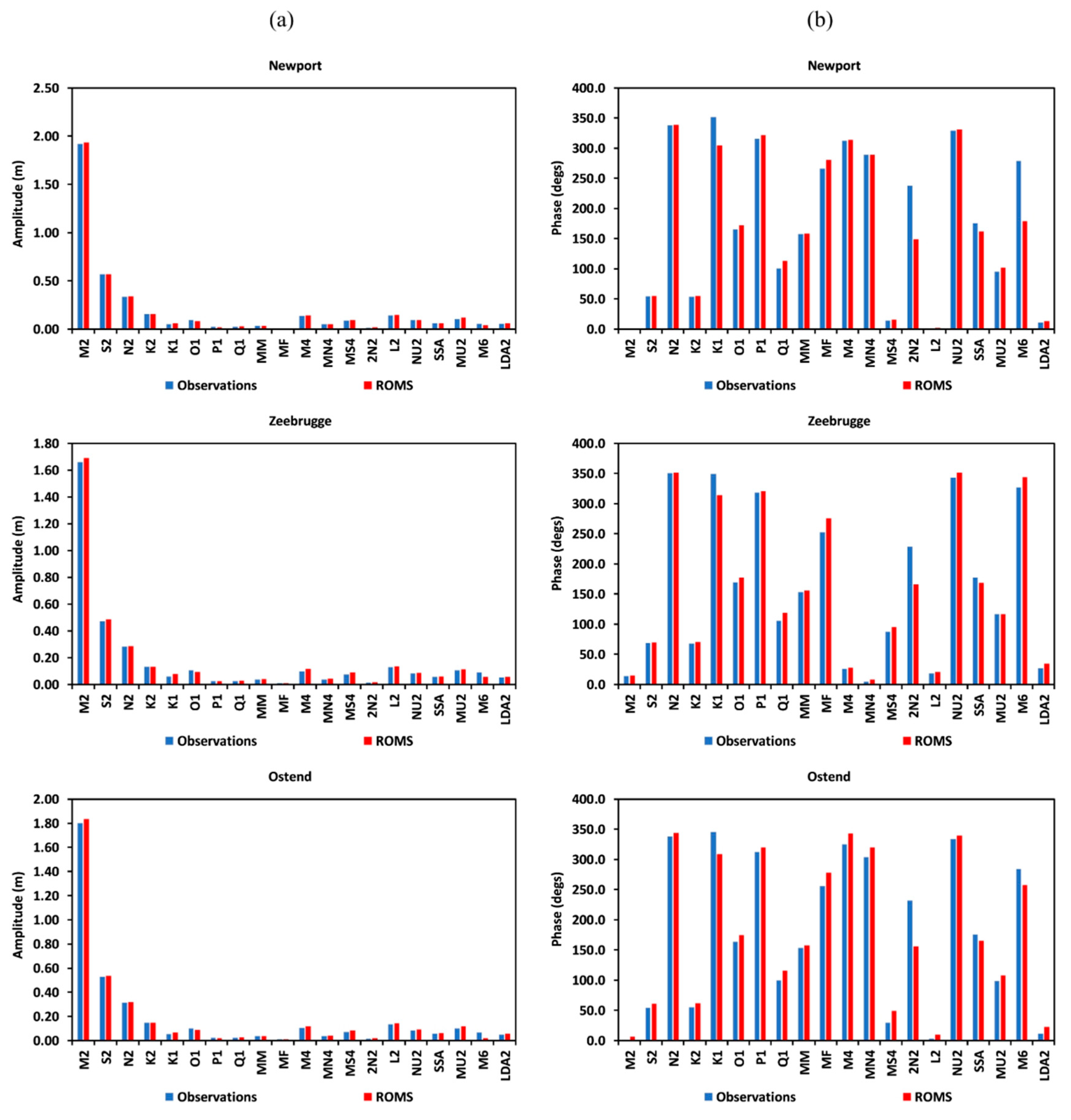
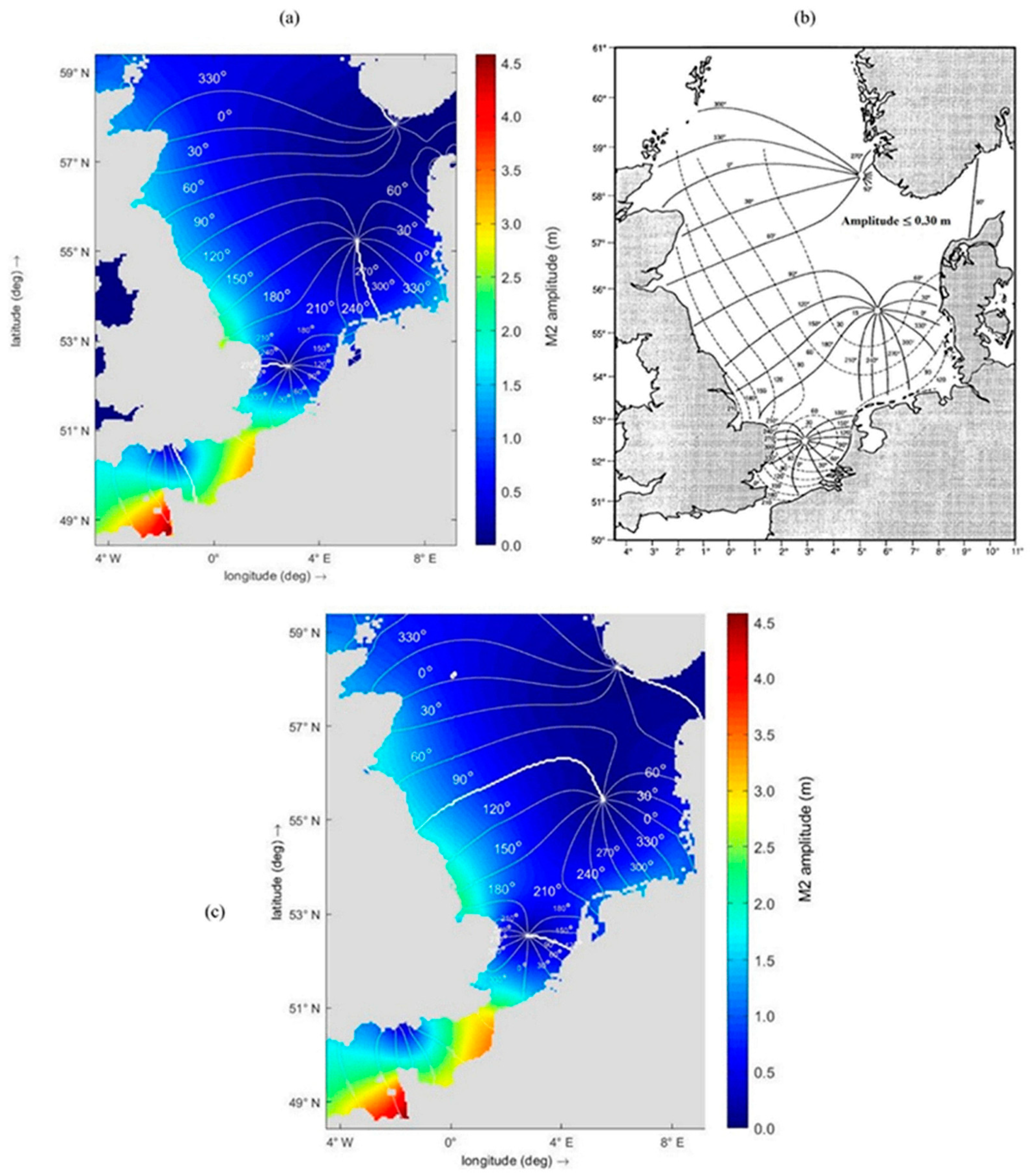
4.2. Model Results for Astronomical Tides
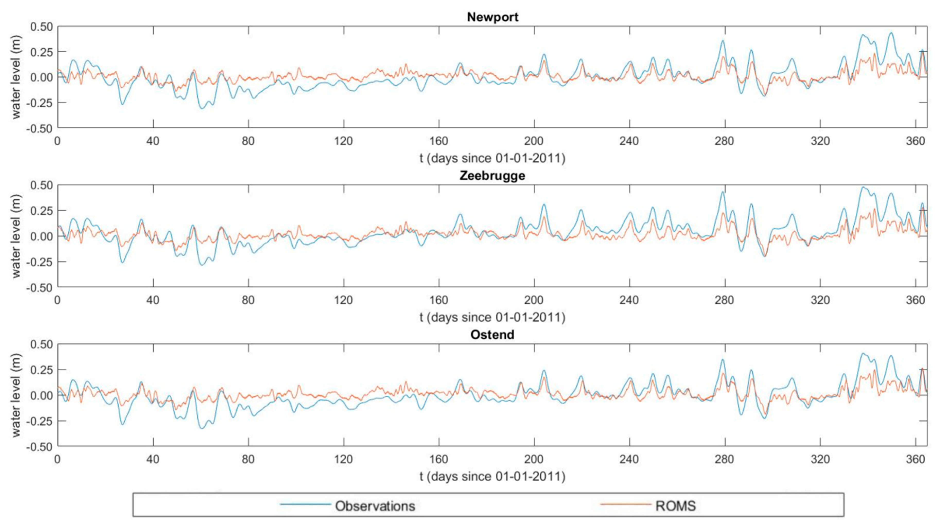
4.3. Model Subtidal Results
4.4. Thermohaline Variation and Atmospheric Surface Fluxes
5. Discussion and Conclusions
Author Contributions
Funding
Institutional Review Board Statement
Informed Consent Statement
Data Availability Statement
Acknowledgments
Conflicts of Interest
References
- Otto, L.; Zimmerman, J.T.F.; Furnes, G.K.; Mork, M.; Saetre, R.; Becker, G. Review of the physical oceanography of the North Sea. Neth. J. Sea Res. 1990. [Google Scholar] [CrossRef]
- Charnock, H.; Dyer, K.R.; Huthnance, J.M.; Liss, P.; Simpson, B.H. Understanding the North Sea System; Springer: Dordrecht, The Netherlands, 2012; ISBN 9789401112369. [Google Scholar]
- Deltares. Delft3D-FLOW. Simulation of Multi-Dimensional Hydrodynamic Flows and Transport Phenomena, Including Sediments User Manual Hydro-Morphodynamics; Version: 3.15.34158; Deltares: Delft, The Netherlands, 2014. [Google Scholar]
- DHI. D.H.I. MIKE 21/MIKE 3 Flow Model FM: Hydrodynamic and Transport Module Scientific Documentation; DHI: Horsholm, Denmark, 2008. [Google Scholar]
- Zijl, F.; Sumihar, J.; Verlaan, M. Application of data assimilation for improved operational water level forecasting on the northwest European shelf and North Sea. Ocean Dyn. 2015, 65, 1699–1716. [Google Scholar] [CrossRef] [Green Version]
- Janin, J.M.; Lepeintre, F.; Péchon, P. TELEMAC-3D: A Finite Element Code to Solve 3D Free Surface Flow Problems. In Computer Modelling of Seas and Coastal Regions; Partridge, P.W., Ed.; Springer: Dordrecht, The Netherlands, 1992; ISBN 978-1-85166-779-6. [Google Scholar]
- Pohlmann, T. Predicting the thermocline in a circulation model of the North sea—Part I: Model description, calibration and verification. Cont. Shelf Res. 1996, 16, 131–146. [Google Scholar] [CrossRef]
- Skogen, M.D.; Søiland, H. A User’s Guide to Norwecom V2.0: The Norwegian Ecological Model System; Fisken og Havet; Institute of Marine Research: Bergen, Norway, 1998. [Google Scholar]
- Proctor, R.; James, I.D. A fine-resolution 3D model of the Southern North Sea. J. Mar. Syst. 1996, 8, 285–295. [Google Scholar] [CrossRef]
- Luyten, P.J.; Jones, J.E.; Proctor, R.; Tabor, A.; Tett, P.; Wild-Allen, K. COHERENS–A Coupled Hydrodynamical-Ecological Model for Regional and Shelf Seas: User Documentation; MUMM Report; Management Unit of the Mathematical Models of the North Sea: Brussels, Belgium, 1999; 914p. [Google Scholar]
- Berg, P.; Poulsen, J.W. Implementation Details for HBM; DMI Technical Report No. 12-11; DMI: Copenhagen, Denmark, 2012. [Google Scholar]
- Lander, J.W.M.; Blokland, P.A.; de Kok, J.M. The Three-Dimensional Shallow Water Model TRIWAQ with a Flexible Vertical Grid Definition; Tech. Rep. RIKZ/OS-96.104x, SIMON A Report 96-01; National Institute for Coastal and Marine Management/RIKZ: The Hague, The Netherlands, 1994. [Google Scholar]
- Lazure, P.; Jegou, A.M. 3D modelling of seasonal evolution of Loire and Gironde plumes on Biscay Bay continental shelf. Oceanol. Acta 1998. [Google Scholar] [CrossRef] [Green Version]
- Delhez, E.; Martin, G. Preliminary results of 3-D baroclinic numerical models of the mesoscale and macroscale circulations on the North-Western Europena Continental Shelf. J. Mar. Syst. 1992. [Google Scholar] [CrossRef]
- Proctor, R.; Damm, P.; Delhez, E.J.M.; Dumas, F.; Gerritsen, H.; de Goede, E.; Jones, J.E.; de Kok, J.; Ozer, J.; Pohlmann, T.; et al. NOMADS—North Sea Model Advection Dispersion Study 2: Assessments of Model Variability (Final Report); Intern. Doc. No. 144; Proudman Oceanogr. Lab.: Liverpool, UK, 2002. [Google Scholar]
- ICES. Flushing times of the North Sea. ICES Coop. Res. Rep. 1983, 123, 159. [Google Scholar]
- Werner, F.E. A field test case for tidally forced flows: A review of the tidal flow forum. In Quantitative Skill Assessment for Coastal Ocean Models, Coastal and Estuarine Studies; Lynch, D.R., Davies, A.M., Eds.; American Geophysical Union: Washington DC, USA, 1995; Volume 47, pp. 269–283. [Google Scholar]
- Hackett, B.; Røed, L.F.; Gjevik, B.; Martinsen, E.A.; Eide, L.I. A review of the Metocean Modeling Project (MOMOP) Part 2: Model validation study. In Quantitative Skill Assessment for Coastal Ocean Models, Coastal and Estuarine Studies; Lynch, D.R., Davies, A.M., Eds.; American Geophysical Union: Washington, DC, USA, 1995; Volume 47, pp. 307–327. [Google Scholar]
- OSPAR. On the use of models in environments in the shipping and offshore industries. In Rep. ASMO Workshop—OSPAR Com. 96; OSPAR: The Hague, The Netherlands, 1996; 75p. [Google Scholar]
- Delhez, É.J.M.; Damm, P.; De Goede, E.; De Kok, J.M.; Dumas, F.; Gerritsen, H.; Jones, J.E.; Ozer, J.; Pohlmann, T.; Rasch, P.S.; et al. Variability of shelf-seas hydrodynamic models: Lessons from the NOMADS2 Project. J. Mar. Syst. 2004. [Google Scholar] [CrossRef]
- Yang, Z.; Zheng, L.; Richardson, P.; Myers, E.; Zhang, A. Model development and hindcast simulations of NOAA’s Integrated Northern Gulf of Mexico Operational Forecast System. J. Mar. Sci. Eng. 2018, 6, 135. [Google Scholar] [CrossRef] [Green Version]
- Lenhart, H.J.; Pohlmann, T. North sea hydrodynamic modelling: A review. Senckenbergiana Marit. 2004. [Google Scholar] [CrossRef]
- Hashemi, M.R.; Neill, S.P.; Davies, A.G. A coupled tide-wave model for the NW European shelf seas. Geophys. Astrophys. Fluid Dyn. 2015. [Google Scholar] [CrossRef] [Green Version]
- Robins, P.E.; Neill, S.P.; Lewis, M.J.; Ward, S.L. Characterising the spatial and temporal variability of the tidal-stream energy resource over the northwest European shelf seas. Appl. Energy 2015. [Google Scholar] [CrossRef] [Green Version]
- Breugem, A.; Verbrugghe, T.; Decrop, B. A continental shelf model in TELEMAC 2D. In Proceedings of the TELEMAC User Conference, Grenoble, France, 15–17 October 2014; Bertrand, O., Coulet, C., Eds.; ARTELIA Eau & Environnement: Echirolles, France, 2014; pp. 43–46. [Google Scholar]
- Delhez, E.J.M.; Carabin, G. Integrated modelling of the Belgian Coastal Zone. Estuar. Coast. Shelf Sci. 2001, 53, 477–491. [Google Scholar] [CrossRef] [Green Version]
- Delhez, E.J.M. Macroscale ecohydrodynamic modeling on the Northwest European continental shelf. J. Mar. Syst. 1998, 16, 171–190. [Google Scholar] [CrossRef]
- Guillou, N.; Chapalain, G.; Thais, L. Three-dimensional modeling of tide-induced suspended transport of seabed multicomponent sediments in the eastern English Channel. J. Geophys. Res. Ocean. 2009. [Google Scholar] [CrossRef] [Green Version]
- Sündermann, J.; Pohlmann, T. A brief analysis of North Sea physics. Oceanologia 2011, 53, 663–689. [Google Scholar] [CrossRef] [Green Version]
- Banner, F.T.; Frederick, T.; Collins, M.B.; Massie, K.S. The North-West European Shelf Seas: The Sea Bed and the Sea in Motion; Elsevier Scientific: Amsterdam, The Netherlands, 1979; ISBN 9780444417343. [Google Scholar]
- Gruwez, V.; Vandebeek, I.; Kisacik, D.; Streicher, M.; Altomare, C.; Suzuki, T.; Verwaest, T.; Kortenhaus, A.; Troch, P. 2D overtopping and impact experiments in shallow foreshore conditions. In Proceedings of the 36th International Conference on Coastal Engineering, Baltimore, ML, USA, 30 July–3 August 2018; Lynett, P., Ed.; ASCE: Reston, VA, USA, 2018; Volume 36, pp. 1–13. [Google Scholar] [CrossRef] [Green Version]
- BSP (Belgian Science Policy). A Flood of Space: Towards a Spatial Structure Plan for Sustainable Management of the North Sea. In Scientific Report GAUFRE Project [CD-ROM]; Belgian Science Policy: Brussels, Belgium, 2005. [Google Scholar]
- de Vries, H.; Breton, M.; de Mulder, T.; Krestenitis, Y.; Ozer, J.; Proctor, R.; Ruddick, K.; Salomon, J.C.; Voorrips, A. A comparison of 2D storm surge models applied to three shallow European seas. Environ. Softw. 1995. [Google Scholar] [CrossRef]
- Di Lorenzo, E. Seasonal dynamics of the surface circulation in the Southern California Current System. Deep. Res. Part II Top. Stud. Oceanogr. 2003. [Google Scholar] [CrossRef]
- Haidvogel, D.B.; Arango, H.G.; Hedstrom, K.; Beckmann, A.; Malanotte-Rizzoli, P.; Shchepetkin, A.F. Model evaluation experiments in the North Atlantic Basin: Simulations in nonlinear terrain-following coordinates. Dyn. Atmos. Ocean. 2000. [Google Scholar] [CrossRef]
- Marchesiello, P.; McWilliams, J.C.; Shchepetkin, A. Equilibrium structure and dynamics of the California current system. J. Phys. Oceanogr. 2003. [Google Scholar] [CrossRef]
- Warner, J.C.; Geyer, W.R.; Lerczak, J.A. Numerical modeling of an estuary: A comprehensive skill assessment. J. Geophys. Res. C Ocean. 2005. [Google Scholar] [CrossRef]
- Warner, J.C.; Sherwood, C.R.; Arango, H.G.; Signell, R.P. Performance of four turbulence closure models implemented using a generic length scale method. Ocean Model. 2005. [Google Scholar] [CrossRef]
- Wilkin, J.L.; Arango, H.G.; Haidvogel, D.B.; Lichtenwalner, C.S.; Glenn, S.M.; Hedström, K.S. A regional ocean modeling system for the Long-term Ecosystem Observatory. J. Geophys. Res. Ocean. 2005. [Google Scholar] [CrossRef] [Green Version]
- Song, Y.; Haidvogel, D. A semi-implicit ocean circulation model using a generalized topography-following coordinate system. J. Comput. Phys. 1994. [Google Scholar] [CrossRef]
- Shchepetkin, A.F.; McWilliams, J.C. The regional oceanic modeling system (ROMS): A split-explicit, free-surface, topography-following-coordinate oceanic model. Ocean Model. 2005. [Google Scholar] [CrossRef]
- Shchepetkin, A.F.; McWilliams, J.C. Correction and commentary for Ocean forecasting in terrain-following coordinates: Formulation and skill assessment of the regional ocean modeling system. J. Comput. Phys. 2009, 227, 3595–3624. [Google Scholar] [CrossRef]
- De Souza, J.M.A.C.; Powell, B.; Castillo-Trujillo, A.C.; Flament, P. The vorticity balance of the ocean surface in Hawaii from a regional reanalysis. J. Phys. Oceanogr. 2015. [Google Scholar] [CrossRef]
- Shchepetkin, A.F.; Mcwilliams, J.C. Quasi-monotone advection schemes based on explicit locally adaptive dissipation. Mon. Weather Rev. 1998. [Google Scholar] [CrossRef]
- Shchepetkin, A.F.; McWilliams, J.C. A method for computing horizontal pressure-gradient force in an oceanic model with a nonaligned vertical coordinate. J. Geophys. Res. C Ocean. 2003. [Google Scholar] [CrossRef]
- Amante, C.; Eakins, B.W. ETOPO1 1 Arc-Minute Global Relief Model: Procedures, Data Sources and Analysis; NOAA Technical Memorandum NESDIS NGDC-24; National Geophysical Data Center: Boulder, CO, USA, 2009. [CrossRef]
- Riley, S.J.; DeGloria, S.D.; Elliot, R. A Terrain Ruggedness Index that Qauntifies Topographic Heterogeneity. Intermt. J. Sci. 1999. [Google Scholar]
- Fairall, C.W.; Bradley, E.F.; Rogers, D.P.; Edson, J.B.; Young, G.S. Bulk parameterization of air-sea fluxes for tropical oceanglobal atmosphere coupled-ocean atmosphere response experiment. J. Geophys. Res. C Ocean. 1996. [Google Scholar] [CrossRef]
- Umlauf, L.; Burchard, H. A generic length-scale equation for geophysical turbulence models. J. Mar. Res. 2003. [Google Scholar] [CrossRef]
- Kantha, L.H.; Clayson, C.A. An improved mixed layer model for geophysical applications. J. Geophys. Res. 1994. [Google Scholar] [CrossRef]
- Chapman, D.C. Numerical treatment of cross-shelf open boundaries in a barotropic coastal ocean model. J. Phys. Ocean. 1985. [Google Scholar] [CrossRef] [Green Version]
- Flather, R.A. A tidal model of the north-west European continental shelf. Mem. Soc. R. Sci. Liege Ser. 1976, 6, 141–164. [Google Scholar]
- Orlanski, I. A simple boundary condition for unbounded hyperbolic flows. J. Comput. Phys. 1976. [Google Scholar] [CrossRef]
- Raymond, W.H.; Kuo, H.L. A radiation boundary condition for multi-dimensional flows. Q. J. R. Meteorol. Soc. 1984. [Google Scholar] [CrossRef]
- Egbert, G.D.; Erofeeva, S.Y. Efficient inverse modeling of barotropic ocean tides. J. Atmos. Ocean. Technol. 2002. [Google Scholar] [CrossRef] [Green Version]
- Egbert, G.D.; Erofeeva, S.Y.; Ray, R.D. Assimilation of altimetry data for nonlinear shallow-water tides: Quarter-diurnal tides of the Northwest European Shelf. Cont. Shelf Res. 2010. [Google Scholar] [CrossRef]
- Carrere, L.; Lyard, F.; Cancet, M.; Guillot, A. FES 2014, a new tidal model on the global ocean with enhanced accuracy in shallow seas and in the Arctic region. In Proceedings of the EGU General Assembly Conference Abstracts, Vienna, Austria, 12–17 April 2015; Volume 17. [Google Scholar]
- Copernicus Climate Change Service (C3S). ERA5: Fifth Generation of ECMWF Atmospheric Reanalyses of the Global Climate. Copernicus Clim. Chang. Serv. Clim. Data Store (CDS). 2017. Available online: https://cds.climate.copernicus.eu/#!/home (accessed on 4 May 2018).
- Hersbach, H.; Dick, L. ERA5 reanalysis is in production. ECMWF Newsl. 2016. Available online: https://www.ecmwf.int/en/newsletter/147/news/era5-reanalysis-production (accessed on 4 May 2018).
- Willmott, C.J. On the validation of models. Phys. Geogr. 1981. [Google Scholar] [CrossRef]
- Pawlowicz, R.; Beardsley, B.; Lentz, S. Classical tidal harmonic analysis including error estimates in MATLAB using TDE. Comput. Geosci. 2002. [Google Scholar] [CrossRef]
- Van Cauwenberghe, L. Harmonic tidal predictions along the Belgian Coast: History and present situation. Infrastruct. Leefmilieu 1999, 1, 373–388. [Google Scholar]
- Pugh, D.T. Tides, Surges and Mean Sea-Level; Wiley: Hoboken, NJ, USA, 1987; ISBN 9780471915058. [Google Scholar]
- Le Provost, C. Theoretical analysis of the structure of the tidal wave’s spectrum in shallow water areas. Mem. Soc. R. Sci. Liege 1976, 6, 97–111. [Google Scholar]
- Dyke, P. Modeling Coastal and Offshore Processes; World Scientific: Singapore, 2007; ISBN 9781860948374. [Google Scholar]
- Liu, W.T.; Katsaros, K.B.; Businger, J.A. Bulk parameterization of air-sea exchanges of heat and water vapor including the molecular constraints at the interface. J. Atmos. Sci. 1979. [Google Scholar] [CrossRef] [Green Version]
- van der Grinten, R.M.; de Vries, J.W.; de Swart, H.E. Impact of wind gusts on sea surface height in storm surge modelling, application to the North Sea. Nat. Hazards 2013. [Google Scholar] [CrossRef] [Green Version]
- Thompson, R.O.R.Y. Low-Pass Filters to Suppress Inertial and Tidal Frequencies. J. Phys. Oceanogr. 1983. [Google Scholar] [CrossRef] [Green Version]
- Svendsen, E.; Sætre, R.; Mork, M. Features of the northern North Sea circulation. Cont. Shelf Res. 1991. [Google Scholar] [CrossRef]


| Stations | Observations | BCS Model | Deviations | ||||||
|---|---|---|---|---|---|---|---|---|---|
| M2 | S2 | N2 | M2 | S2 | N2 | M2 | S2 | N2 | |
| Newport | 1.92 | 0.57 | 0.33 | 1.94 | 0.57 | 0.34 | 0.02 | 0.00 | 0.01 |
| Westhinder | 1.69 | 0.50 | 0.29 | 1.68 | 0.49 | 0.29 | −0.01 | −0.01 | 0.00 |
| Zeebrugge | 1.66 | 0.47 | 0.28 | 1.69 | 0.49 | 0.29 | 0.03 | 0.02 | 0.01 |
| Ostend | 1.80 | 0.53 | 0.31 | 1.83 | 0.53 | 0.32 | 0.03 | 0.00 | 0.01 |
| SW | 1.58 | 0.43 | 0.29 | 1.65 | 0.47 | 0.28 | 0.07 | 0.04 | −0.01 |
| BVH | 1.62 | 0.46 | 0.28 | 1.67 | 0.48 | 0.28 | 0.05 | 0.02 | 0.00 |
| A2 | 1.65 | 0.47 | 0.28 | 1.69 | 0.49 | 0.29 | 0.04 | 0.02 | 0.01 |
| Wandelaar | 1.61 | 0.46 | 0.27 | 1.66 | 0.48 | 0.28 | 0.05 | 0.02 | 0.01 |
| Stations | Observations | BCS Model | Deviations | ||||||
|---|---|---|---|---|---|---|---|---|---|
| M2 | S2 | N2 | M2 | S2 | N2 | M2 | S2 | N2 | |
| Newport | 0.7 | 54.6 | 338.0 | 1.3 | 55.3 | 338.3 | 0.60 | 0.70 | 0.30 |
| Westhinder | 353.8 | 47.3 | 329.9 | 358.1 | 51.8 | 334.4 | 4.30 | 4.50 | 4.50 |
| Zeebrugge | 14.0 | 68.7 | 350.9 | 14.7 | 69.9 | 351.5 | 0.70 | 1.20 | 0.60 |
| Ostend | 0.5 | 54.4 | 337.7 | 6.8 | 61.3 | 343.7 | 6.30 | 6.90 | 6.00 |
| SW | 19.2 | 74.1 | 359.3 | 17.6 | 73.1 | 354.4 | −1.60 | −1.00 | −4.90 |
| BVH | 14.8 | 69.8 | 352.0 | 15.1 | 70.4 | 351.9 | 0.30 | 0.60 | −0.10 |
| A2 | 11.5 | 66.1 | 348.6 | 13.1 | 68.1 | 349.8 | 1.60 | 2.00 | 1.20 |
| Wandelaar | 10.0 | 64.4 | 346.8 | 11.8 | 66.7 | 348.5 | 1.80 | 2.30 | 1.70 |
| Tidal Stations | Astronomical Tides | Atmospheric Forcing | |||
|---|---|---|---|---|---|
| MAE (m) | RMSE (m) | Cor | S.I. | RMSE (m) | |
| 22. Newport | 0.081 | 0.100 | 0.998 | 0.999 | 0.114 |
| 23. Westhinder | 0.104 | 0.121 | 0.996 | 0.998 | 0.110 |
| 24. Zeebrugge | 0.073 | 0.091 | 0.998 | 0.999 | 0.114 |
| 25. Ostend | 0.156 | 0.179 | 0.992 | 0.996 | 0.118 |
| 26. Scheur Wielingen | 0.089 | 0.116 | 0.997 | 0.998 | 0.118 |
| 27. Bol Van Heist | 0.073 | 0.090 | 0.998 | 0.999 | 0.125 |
| 28. A2 | 0.080 | 0.100 | 0.997 | 0.998 | 0.121 |
| 29. Wandelaar | 0.082 | 0.102 | 0.997 | 0.998 | 0.126 |
| 46. Stavanger | 0.026 | 0.033 | 0.969 | 0.984 | 0.081 |
| 44. Hanstholm | 0.031 | 0.037 | 0.947 | 0.954 | 0.051 |
| 42. Hörnum | 0.112 | 0.132 | 0.993 | 0.989 | 0.075 |
| 35. Platform A12 | 0.081 | 0.098 | 0.894 | 0.944 | 0.133 |
| 20. Calais | 0.210 | 0.259 | 0.991 | 1.000 | 0.196 |
| 11. Bournemouth | 0.181 | 0.221 | 0.829 | 0.908 | 0.153 |
| 4. Whitby | 0.128 | 0.151 | 0.959 | 0.996 | 0.203 |
| 2. Aberdeen | 0.129 | 0.161 | 0.989 | 0.994 | 0.181 |
| Tidal Stations | Atmospheric Forcing—Bulk Formulation [48] | Atmospheric Forcing—ECMWF | ||
|---|---|---|---|---|
| RMSE (m) | Cor | RMSE (m) | Cor | |
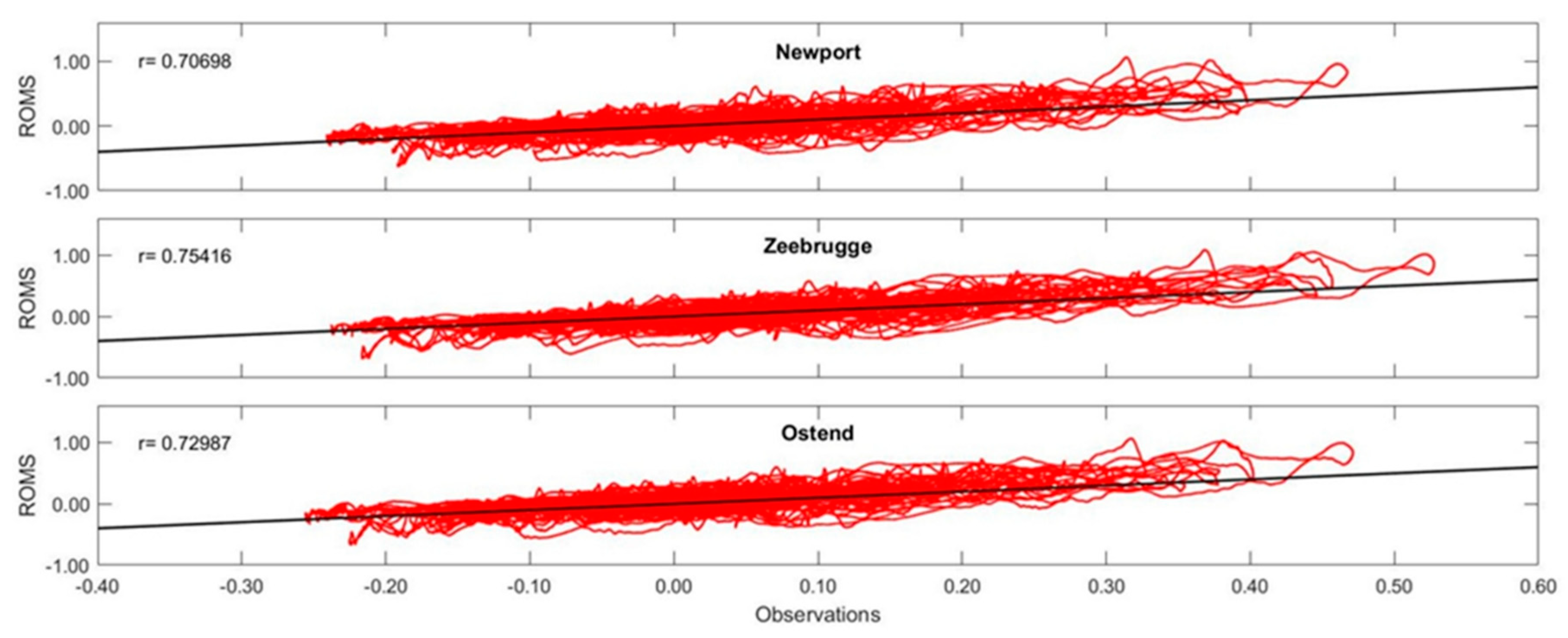
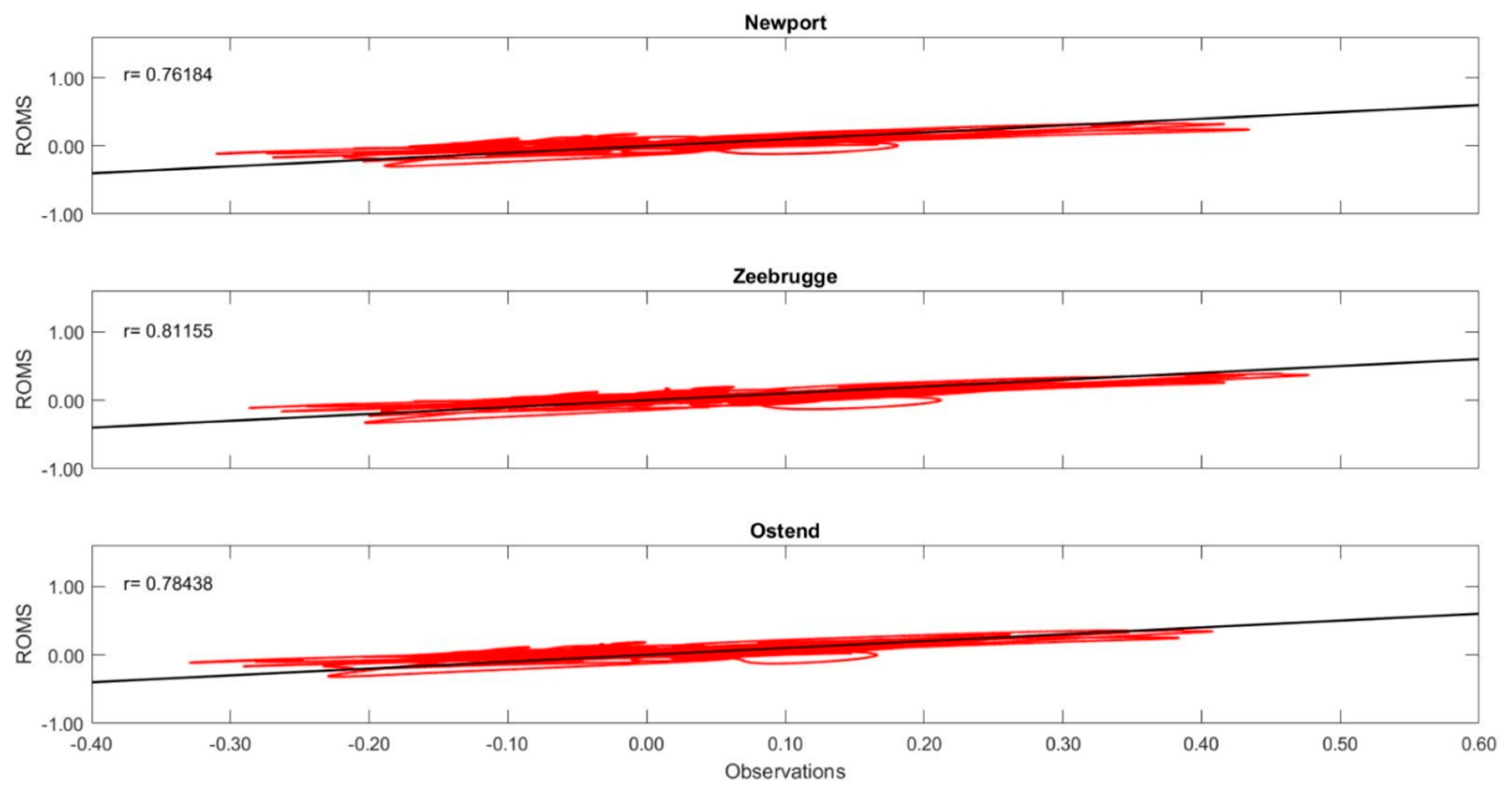
| 22. Newport | 0.114 | 0.707 | 0.085 | 0.762 |
| 23. Westhinder | 0.110 | 0.668 | 0.085 | 0.696 |
| 24. Zeebrugge | 0.114 | 0.754 | 0.106 | 0.812 |
| 25. Ostend | 0.118 | 0.730 | 0.084 | 0.784 |
| 26. Scheur Wielingen | 0.118 | 0.587 | 0.094 | 0.653 |
| 27. Bol Van Heist | 0.125 | 0.756 | 0.104 | 0.813 |
| 28. A2 | 0.121 | 0.729 | 0.094 | 0.790 |
| 29. Wandelaar | 0.126 | 0.740 | 0.110 | 0.790 |
| 46. Stavanger | 0.081 | 0.060 | 0.031 | 0.122 |
| 44. Hanstholm | 0.051 | 0.032 | 0.039 | 0.045 |
| 42. Hörnum | 0.075 | 0.319 | 0.029 | 0.885 |
| 35. Platform A12 | 0.133 | 0.086 | 0.032 | 0.635 |
| 20. Calais | 0.196 | 0.173 | 0.195 | 0.173 |
| 11. Bournemouth | 0.153 | 0.172 | 0.041 | 0.409 |
| 4. Whitby | 0.203 | 0.220 | 0.088 | 0.451 |
| 2. Aberdeen | 0.181 | 0.015 | 0.180 | 0.099 |
Publisher’s Note: MDPI stays neutral with regard to jurisdictional claims in published maps and institutional affiliations. |
© 2021 by the authors. Licensee MDPI, Basel, Switzerland. This article is an open access article distributed under the terms and conditions of the Creative Commons Attribution (CC BY) license (http://creativecommons.org/licenses/by/4.0/).
Share and Cite
Klonaris, G.; Van Eeden, F.; Verbeurgt, J.; Troch, P.; Constales, D.; Poppe, H.; De Wulf, A. ROMS Based Hydrodynamic Modelling Focusing on the Belgian Part of the Southern North Sea. J. Mar. Sci. Eng. 2021, 9, 58. https://doi.org/10.3390/jmse9010058
Klonaris G, Van Eeden F, Verbeurgt J, Troch P, Constales D, Poppe H, De Wulf A. ROMS Based Hydrodynamic Modelling Focusing on the Belgian Part of the Southern North Sea. Journal of Marine Science and Engineering. 2021; 9(1):58. https://doi.org/10.3390/jmse9010058
Chicago/Turabian StyleKlonaris, Georgios, Frans Van Eeden, Jeffrey Verbeurgt, Peter Troch, Denis Constales, Hans Poppe, and Alain De Wulf. 2021. "ROMS Based Hydrodynamic Modelling Focusing on the Belgian Part of the Southern North Sea" Journal of Marine Science and Engineering 9, no. 1: 58. https://doi.org/10.3390/jmse9010058