Considerations on the aggregate monotonicity of the nucleolus and the core-center

Abstract

Even though aggregate monotonicity appears to be a reasonable requirement for solutions on the domain of convex games, there are well known allocations, the nucleolus for instance, that violate it. It is known that the nucleolus is aggregate monotonic on the domain of essential games with just three players. We provide a simple direct proof of this fact, obtaining an analytic formula for the nucleolus of a three-player essential game. We also show that the core-center, the center of gravity of the core, satisfies aggregate monotonicity for three-player balanced games. The core is aggregate monotonic as a set-valued solution, but this is a weak property. In fact, we show that the core-center is not aggregate monotonic on the domain of convex games with at least four players. Our analysis allows us to identify a subclass of bankruptcy games for which we can obtain analytic formulae for the nucleolus and the core-center. Moreover, on this particular subclass, aggregate monotonicity has a clear interpretation in terms of the associated bankruptcy problem and both the nucleolus and the core-center satisfy it.

Appendix

1.1 Proof of Proposition 3.3

Let $N=\{1,2,3\}$ and $v=(v_{-3},v_{-2}, v_{-1}, E) \in {\mathcal {E}}_{0^+}^N$ so that $0\le v_{-3}\le v_{-2} \le v_{-1}$ and $E\ge 0$. First, let us assume that v is a balanced game, that is, $E\ge \alpha =\max \bigl \{v_{-1}, \tfrac{1}{2}( v_{-1}+v_{-2}+v_{-3}) \bigr \}$. Clearly, for 3-player balanced games the 1-nucleolus and the nucleolus coincide, so $\eta (v)=\eta ^1(v)$. Estévez-Fernández et al. (2017) prove⁵ that if $v\in \mathcal {MB}^N$ and we define the vector $d=(d_1,d_2,d_3)$ as $d_i=E-v_{-i}$ for all $i\in N$ then $(E,d)\in \mathcal {P^N}$ and the 1-nucleolus of v coincides with the Talmud rule of (E, d), i.e., $\eta ^1(v)=T(E,d)$. Then, the formula for $\eta _1(v)$ is straightforward. Moreover, Estévez-Fernández et al. (2017) show that the 1-nucleolus satisfies first agent consistency:

• If $v\in {\mathcal {B}}^N$ and we consider the game $v_{1,\eta _1(v)} \in {\mathcal {B}}^{\{2,3\}}$ defined, for all $S\subset \{2,3\}$, by:

  $$\begin{aligned} v_{1,\eta _1(v)}(S)= {\left\{ \begin{array}{ll} 0 &{} \text {if } S=\emptyset \\ \max \bigl \{ 0, v(S \cup \{1\})-\eta _1(v) \bigr \} &{} \text {if } |S|=1\\ v(N)-\eta _1(v) &{} \text {if } S=\{2,3\} \end{array}\right. } \end{aligned}$$

  then $\eta _i(v)=\eta _i(v_{1,\eta _1(v)})$ for $i\in \{2,3\}$.

Applying first agent consistency it is easy to deduce the expressions for $\eta _2(v)$ and $\eta _3(v)$. In fact,

$$\begin{aligned} \eta _1(v)&= {\left\{ \begin{array}{ll} \tfrac{1}{3}\bigl ( E+v_{-2}+v_{-3}-2v_{-1} \bigr ) &{} \text {if } \alpha \le E \le 2(v_{-2}+v_{-3})-v_{-1}\\ \tfrac{1}{2}\bigl ( E-v_{-1} \bigr ) &{} \text {if } 2(v_{-2}+v_{-3})-v_{-1} \le E \le 3v_{-1}\\ \tfrac{1}{3}E &{} \text {if } 3v_{-1}\le E \end{array}\right. } \\ \eta _2(v)&= {\left\{ \begin{array}{ll} \tfrac{1}{3}\bigl ( E+v_{-1}-2v_{-2}+v_{-3}\bigr ) &{} \text {if } \alpha \le E \le 2(v_{-2}+v_{-3})-v_{-1}\\ \tfrac{1}{4}\bigl ( E+v_{-1} -2v_{-2}+2v_{-3}\bigr ) &{} \text {if } 2(v_{-2}+v_{-3})-v_{-1} \le E \le v_{-1}+2v_{-3}\\ \tfrac{1}{2}\bigl ( E-v_{-2} \bigr ) &{} \text {if } v_{-1}+2v_{-3} \le E\le v_{-1}+2v_{-2} \\ \tfrac{1}{4}\bigl ( E+v_{-1} \bigr ) &{} \text {if } v_{-1}+2v_{-2} \le E\le 3v_{-1}\\ \tfrac{1}{3}E &{} \text {if } 3v_{-1}\le E \end{array}\right. } \\ \eta _3(v)&= {\left\{ \begin{array}{ll} \tfrac{1}{3}\bigl ( E+v_{-1}+v_{-2}-2v_{-3} \bigr ) &{} \text {if } \alpha \le E \le 2(v_{-2}+v_{-3})-v_{-1}\\ \tfrac{1}{4}\bigl ( E+v_{-1} +2v_{-2}-2v_{-3}\bigr ) &{} \text {if } 2(v_{-2}+v_{-3})-v_{-1} \le E \le v_{-1}+2v_{-3} \\ \tfrac{1}{2}\bigl ( v_{-1}+v_{-2} \bigr ) &{} \text {if } v_{-1}+2v_{-3} \le E\le v_{-1}+2v_{-2} \\ \tfrac{1}{4}\bigl ( E+v_{-1} \bigr ) &{} \text {if } v_{-1}+2v_{-2} \le E\le 3v_{-1}\\ \tfrac{1}{3}E &{} \text {if } 3v_{-1}\le E \end{array}\right. } \end{aligned}$$

Next, we compute the nucleolus of an essential zero-normalized game that is not balanced. So, let $v\in {\mathcal {E}}_{0^+}^N$ such that $v\not \in {\mathcal {B}}^N$, that is, $\max \bigl \{ v_{-1}-E, v_{-3}+v_{-2}+v_{-1}-2E \bigr \}>0$. Maschler et al. (1979) present a method of finding the nucleolus that requires to solve a sequence of minimization linear programming problems. In the first step, the procedure finds all the imputations $x\in I(v)$ whose maximal excess $\theta _1(x)$ is as small as possible. So, let $\varepsilon _1(v)=\underset{x\in I(v)}{\min }\ \underset{S\in \Sigma ^0}{\max }\ e(x,S)$. Clearly $\varepsilon _1(v)>0$ since $C(v)=\emptyset$ so $\varepsilon _1(v)$ is the optimum value of the mathematical programming problem:

Denote by $X^1=\{ x \in I(v): e(S,x)\le \varepsilon _1(v) \text { for all } S\in 2^N \}$ the set of imputations at which the minimum of the excesses is attained. Let $\Sigma _1=\{ S\in \Sigma ^0: e(S,x)=\varepsilon _1(v) \text { for all } x\in X^1\}$ be the set of all coalitions at which the maximal excess $\varepsilon _1(v)$ is attained at all $x\in X^1$, and let $\Sigma ^1=\{ S\in \Sigma ^0: S\not \in \Sigma _1\}=\Sigma ^0\backslash \Sigma _1$. Denote $\varepsilon ^*=\max \bigl \{v_{-1}-E, \tfrac{1}{3} (v_{-3}+v_{-2}+v_{-1}-2E) \bigr \}$. Since $v\not \in {\mathcal {B}}^N$ we have that $\varepsilon ^*>0$. Now, if $(x_1,x_2,\varepsilon _1)$ is a feasible solution of ($P_1$) then $0\le \varepsilon _1 +E-v_{-1}$, $0\le \varepsilon _1 +E-v_{-2}$ and $v_{-3}-\varepsilon _1\le E$ so $\varepsilon _1\ge v_{-1}-E\ge v_{-2}-E\ge v_{-3}-E$. Moreover, $x_1+x_2\le 2\varepsilon _1+2E-v_{-1}-v_{-2}$ and then $v_{-3}-\varepsilon _1\le 2\varepsilon _1+2E-v_{-1}-v_{-2}$ which implies that $\varepsilon _1\ge \tfrac{1}{3}\bigl (v_{-3}+v_{-2}+v_{-1}-2E \bigr )$. As a consequence $\varepsilon _1(v)\ge \varepsilon ^*$.

Suppose that $\varepsilon ^*=\tfrac{1}{3} (v_{-3}+v_{-2}+v_{-1}-2E)$. Then $(x^*_1,x^*_2,\varepsilon _1^*)=\tfrac{1}{3}\bigl (E+v_{-3}+v_{-2}-2v_{-1}, E+v_{-3}-2v_{-2}+v_{-1},v_{-3}+v_{-2}+v_{-1}-2E\bigr )$ is a feasible solution of ($P_1$), so $\varepsilon _1(v)=\tfrac{1}{3} (v_{-3}+v_{-2}+v_{-1}-2E)$. But $(x^*_1,x^*_2,\varepsilon _1^*)$ is the only feasible solution at which the minimum $\varepsilon _1^*$ is attained, so $X^1=\{ (x_1^*,x_2^*,E-x_1^*-x_2^*) \}$. Therefore, if $\varepsilon ^*=\tfrac{1}{3} (v_{-3}+v_{-2}+v_{-1}-2E)$ we have that $\eta (v)=(x_1^*,x_2^*,E-x_1^*-x_2^*)$.

Now, $\varepsilon ^*=v_{-1}-E$ if and only if $E\le 2v_{-1}-v_{-2}-v_{-3}$. If this condition holds, we distinguish three cases:

• 1. If $E<v_{-1}-v_{-2}\le v_{-1}-v_{-3}$ then $(0,x_2,\varepsilon _1^*)$ is a feasible solution of ($P_1$) for all $0\le x_2 \le E$. Therefore, $\varepsilon _1(v)=v_{-1}-E$, $X^1=\{(0,x_2,E-x_2):0\le x_2 \le E\}$, and $\Sigma _1=\{ \{2,3\} \}$.

• 2. If $v_{-1}-v_{-2}\le E\le v_{-1}-v_{-3}$ then $(0,x_2,\varepsilon _1^*)$ is a feasible solution of ($P_1$) for all $0\le x_2 \le v_{-1}-v_{-2}$. Therefore, $\varepsilon _1(v)=v_{-1}-E$, $X^1=\{(0,x_2,E-x_2):0\le x_2 \le v_{-1}-v_{-2}\}$, and $\Sigma _1=\{ \{2,3\} \}$.

• 3. If $v_{-1}-v_{-2}\le v_{-1}-v_{-3}\le E$ then $(0,x_2,\varepsilon _1^*)$ is a feasible solution of ($P_1$) for all $E-(v_{-1}-v_{-3} )\le x_2 \le v_{-1}-v_{-2}$. Therefore, $\varepsilon _1(v)=v_{-1}-E$, $X^1=\{(0,x_2,E-x_2):E-v_{-1}+v_{-3}\le x_2 \le v_{-1}-v_{-2}\}$, and $\Sigma _1=\{ \{2,3\} \}$.

Therefore, if $\varepsilon ^*=v_{-1}-E$, we have to proceed with the second step in the method described in Maschler et al. (1979), that is, we must find the minimum second-largest excess. Let $\varepsilon _2(v)=\underset{x\in X^1}{\min }\ \underset{S\in \Sigma ^1}{\max }\ e(x,S)$. Denote $X^2=\{ x \in X^1: e(S,x)\le \varepsilon _2(v) \text { for all } S\in \Sigma ^1 \}$, $\Sigma _2=\{ S\in \Sigma ^1: e(S,x)=\varepsilon _2(v) \text { for all } x\in X^2\}$, and $\Sigma ^2=\{ S\in \Sigma ^1: S\not \in \Sigma _2\}=\Sigma ^1\backslash \Sigma _2$. Then, $\varepsilon _2(v)$ is the value of the following linear program:

$$\begin{aligned} \begin{array}{ll} \text {minimize} &{} \varepsilon _2\\ \text {subject to}: &{} e(S,x)= v_{-1}-E, \text { for all } S\in \Sigma _1\\ &{} e(S,x)\le \varepsilon _2, \text { for all }S\in \Sigma ^1\\ &{} x_1 +x_2 +x_3=E\\ &{} x_1 \ge 0, x_2 \ge 0, x_3 \ge 0 \end{array} \end{aligned}$$

But if $x=(x_1,x_2,x_3)\in X^1$ then $x_1=0$. Since $\{1\}\not \in \Sigma _1$ and $e(\{1\},x)=0$, we have that $\varepsilon _2(v)\ge 0$. As a consequence, $\varepsilon _2(v)$ is the solution of the reduced linear program with unkowns $x_2,\varepsilon _2$:

If $(x_2,\varepsilon _2)$ is a feasible solution of ($P_2$) then $v_{-3}- \varepsilon _2 \le E-v_{-2}+\varepsilon _2$, that is, $\varepsilon _2 \ge \tfrac{1}{2}(v_{-3}+v_{-2}-E)$. So $\varepsilon _2(v) \ge \varepsilon _2^*=\max \{ 0, \tfrac{1}{2}(v_{-3}+v_{-2}-E)\}$. The intersection of the straight lines $x_2+\varepsilon _2= v_{-3}$ and $x_2-\varepsilon _2= E-v_{-2}$ is the point $({\hat{x}}_2,{\hat{\varepsilon }}_2)=\bigl ((\tfrac{1}{2}(E+v_{-3}-v_{-2}),\tfrac{1}{2}(v_{-3}+v_{-2}-E)\bigr )$. Clearly ${\hat{x}}_2\ge 0$ if and only if $E\ge v_{-2}-v_{-3}$ and ${\hat{\varepsilon }}_2\ge 0$ whenever $E\le v_{-2}+v_{-3}$. Therefore, we distinguish three cases:

• 1. If $0\le E\le v_{-2}-v_{-3}$ then the constraint set is $\{(x_2,\varepsilon _2)\in {\mathbb {R}}^2: 0\le x_2\le E, x_2-\varepsilon _2\le E-v_{-2}\}$ and has two extreme points: $(0,v_{-2}-E)$ and $(E,v_{-2})$. So the optimum feasible solution of ($P_2$) is $(x_2^*,\varepsilon _2^*)=(0,v_{-2}-E)$. Therefore $\varepsilon _2(v)=v_{-2}-E\ge 0$ and $\eta (v)=(0,0,E)$.

• 2. If $v_{-2}-v_{-3}\le E\le v_{-2}+v_{-3}$ then the constraint set has three extreme points: $(0,v_{-3})$, $(E,v_{-2})$, and $({\hat{x}}_2,{\hat{\varepsilon }}_2)$. Clearly, $({\hat{x}}_2,{\hat{\varepsilon }}_2)$ is the optimum feasible solution of ($P_2$). Therefore $\varepsilon _2(v)=\tfrac{1}{2}(v_{-3}+v_{-2}-E)$ and $\eta (v)=\bigl (0,\tfrac{E+v_{-3}-v_{-2}}{2}, \tfrac{E-v_{-3}+v_{-2}}{2}\bigr )$.

• 3. If $E> v_{-3}+v_{-2}$ then $\varepsilon _2^*=0$. So $(x_2,0)$ is a feasible solution of ($P_2$) for all $v_{-3}\le x_2 \le E-v_{-2}$. Therefore, $\varepsilon _2(v)=0$, $X^2=\{(0,x_2,E-x_2):v_{-3}\le x_2 \le E-v_{-2}\}$, and $\Sigma _2=\{ \{1\} \}$. Let $\varepsilon _3(v)=\underset{x\in X^2}{\min }\ \underset{S\in \Sigma ^2}{\max }\ e(x,S)$ be the minimum third-largest excess. Then, $\varepsilon _3(v)$ is the solution of the linear program with unkowns $x_2,\varepsilon _3$:

  

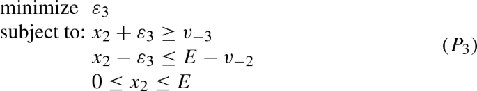
  Observe that the only difference between the linear programs ($P_2$) and ($P_3$) is the positivity constraint $\varepsilon \ge 0$. Then, the constraint set of ($P_3$) has three extreme points: $(0,v_{-3})$, $(E,v_{-2})$, and $({\hat{x}}_2,{\hat{\varepsilon }}_2)$. Since $\tfrac{1}{2}(v_{-3}+v_{-2}-E)<0$, the optimal feasible solution is $({\hat{x}}_2,{\hat{\varepsilon }}_2)$. Therefore $\varepsilon _3(v)=\tfrac{1}{2}(v_{-3}+v_{-2}-E)$ and $\eta (v)=\bigl (0,\tfrac{E+v_{-3}-v_{-2}}{2}, \tfrac{E-v_{-3}+v_{-2}}{2}\bigr )$.

1.2 Proof of Proposition 4.2

Let $N=\{1,2,3\}$ and $v=(v_{-3},v_{-2},v_{-1},E)\in \mathcal {MB}^N$ such that $v_{-3}\le v_{-2} \le v_{-1}$ and $\alpha =\max \bigl \{0, v_{-1}, \tfrac{1}{2}( v_{-1}+v_{-2}+v_{-3}) \bigr \}\le E$. Let $w\in {\mathcal {C}}^N$ be the exact envelope of v, i.e., $w=v^e$, so $C(v)=C(w)$ and $\mu (v)=\mu (w)$. We identify the convex game $w\in {\mathcal {C}}^N$ with the vector

$$\begin{aligned} \bigl (w(\{1\}), w(\{2\}), w(\{3\}), w(\{1,2\}), w(\{1,3\}), w(\{2,3\}), w(N)\bigr )\in {\mathbb {R}}^7. \end{aligned}$$

Let $a=\bigl (w(\{i\}) \bigr )_{i\in N}$ and $w^0=(w^0_{-3},w^0_{-2},w^0_{-1},w^0(N)) \in \mathcal {MC}^N$ be the zero-normalization of w so that $w=a+w^0$. Since $w_0\in \mathcal {MC}^N$, from the analytic formula given in Proposition 4.1, we can obtain $\mu (w^0)$. But having into account that $\mu (v)=\mu (w)=a+\mu (w^0)$, we can derived the following expressions for $\mu (v)$:

• 1. $v_{-k}\ge 0$ for all $k \in N$.

  • If $E\in [\alpha ,v_{-3}+v_{-2}]$ then $w=(v_{-3}+v_{-2}-E,v_{-3}+v_{-1}-E,v_{-2}+v_{-1}-E,v_{-3},v_{-2},v_{-1},E)\in {\mathcal {C}}^N$ and $w^0=\bigl (2E- {\sum _{i\in N}} v_{-i} , 2E- \underset{i\in N}{\sum } v_{-i} , 2E- {\sum _{i\in N}} v_{-i} ,2(2E- {\sum _{i\in N}} v_{-i} )\bigr )\in \mathcal {MC}^N$. Therefore $\mu _i(v)=\mu _i(w)= \mu _i(w_0)+{\sum _{k\ne i}} v_{-k}-E$ for all $i\in N$. Moreover, $\mu _1(v) \le \mu _2(v) \le \mu _3(v)$.

  • If $E\in [v_{-3}+v_{-2},v_{-3}+v_{-1}]$ then $w=(0,v_{-3}+v_{-1}-E,v_{-2}+v_{-1}-E,v_{-3},v_{-2},v_{-1},E) \in {\mathcal {C}}^N$ and $w^0=\bigl (E-v_{-1}, E-v_{-1}, 2E-{\sum _{i\in N}} v_{-i} ,3E-v_{-3}-v_{-2}-2v_{-1}\bigr )\in \mathcal {MC}^N$. In this case, $\mu _1(v)=\mu _1(w)= \mu _1(w_0)$, $\mu _2(v)=\mu _2(w)= \mu _2(w_0)+v_{-3}+v_{-1}-E$ and $\mu _3(v)=\mu _3(w)= \mu _3(w_0)+v_{-2}+v_{-1}-E$. We have that $\mu _1(v) \le \mu _2(v) \le \mu _3(v)$.

  • If $E\in [v_{-3}+v_{-1},v_{-2}+v_{-1}]$ then $w=(0,0,v_{-2}+v_{-1}-E,v_{-3},v_{-2},v_{-1},E) \in {\mathcal {C}}^N$ and $w^0=\bigl (v_{-3}, E-v_{-1}, E-v_{-2},2E-v_{-2}-v_{-1}\bigr )\in \mathcal {MC}^N$. Now, $\mu _1(v)=\mu _1(w)= \mu _1(w_0)$, $\mu _2(v)=\mu _2(w)= \mu _2(w_0)$ and $\mu _3(v)=\mu _3(w)= \mu _3(w_0)+v_{-2}+v_{-1}-E$. Again, $\mu _1(v) \le \mu _2(v) \le \mu _3(v)$.

  • If $E\in [v_{-2}+v_{-1},+\infty )$ then $w^0=w$, and $\mu (v)=\mu (w)=\mu (w^0)$.

• 2. There is $k \in N$ such that $v_{-k}\le 0$.

  • If $v_{-1}\le 0$ then $w=w^0=\bigl (0,0,0,E \bigr )$ and $\mu _i (v)=\mu _i (w_0)=\frac{E}{3}$ for all $i \in N$.

  • If $v_{-2}\le 0 \le v_{-1}$ then $w=w^0=\bigl (0,0, v_{-1},E \bigr )$ and $\mu _1 (v)=\tfrac{E^3-3Ev_{-1}^2+2v_{-1}^3}{3(E^2-v_{-1}^2)} =\tfrac{E^2+Ev_{-1}-2v_{-1}^2}{3(E+v_{-1})}=\tfrac{E}{3}-\tfrac{2v_{-1}^2}{3(E+v_{-1})}$, $\mu _2 (v) =\mu _3(v)=\tfrac{E^3-v_{-1}^3}{3(E^2-v_{-1}^2)} =\tfrac{(E-v_{-1})(E^2+Ev_{-1}+v_{-1}^2)}{3(E-v_{-1})(E+v_{-1})}=\tfrac{E^2+Ev_{-1}+v_{-1}^2}{3(E+v_{-1})}=\tfrac{E}{3}+\tfrac{v_{-1}^2}{3(E+v_{-1})}$.

  • If $v_{-3}\le 0 \le v_{-2}$ and $E\le v_{-2}+v_{-1}$ then $w=(0,0,v_{-2}+v_{-1}-E,0,v_{-2},v_{-1},E)$ and $w_0= \bigl (0,E-v_{-1},E-v_{-2},2E-v_{-2}-v_{-1} \bigr )$. Therefore, $\mu _1 (v)=\mu _1 (w_0)=\tfrac{E-v_{-1}}{2}$, $\mu _2 (v)=\mu _2 (w_0)=\tfrac{E-v_{-2}}{2}$, and $\mu _3 (v)=\mu _3 (w_0)+v_{-2}+v_{-1}-E=\tfrac{v_{-2}+v_{-1}}{2}$.

  • If $v_{-3}\le 0 \le v_{-2}$ and $v_{-2}+v_{-1}\le E$, then $w=w^0=\bigl (0,v_{-2}, v_{-1},E \bigr )$. As a consequence $\mu _1 (v)=\tfrac{E^3 - 3Ev_{-1}^2 - v_{-2}^3 + 2 v_{-1}^3}{3( E^2 -v_{-2}^2- v_{-1}^2)}$, $\mu _2 (v)=\tfrac{E^3 - 3Ev_{-2}^2 - v_{-1}^3 + 2 v_{-2}^3}{3( E^2 -v_{-2}^2- v_{-1}^2)}$, and $\mu _3 (v)=\tfrac{E^3 -v_{-2}^3- v_{-1}^3}{3( E^2 -v_{-2}^2- v_{-1}^2)}$.

  Note that in all the cases we have that $\mu _1(v)\le \mu _2(v) \le \mu _3(v)$.

1.3 Proof of Theorem 4.3

Fix a vector $(v_{-3},v_{-2}, v_{-1}) \in {\mathbb {R}}^3$ such that $v_{-3}\le v_{-2} \le v_{-1}$ and let $\alpha =\max \bigl \{0, v_{-1}, \tfrac{1}{2}( v_{-1}+v_{-2}+v_{-3}) \bigr \}$. For each $i\in N$ consider the function $\mu _i: [\alpha ,+\infty )\rightarrow {\mathbb {R}}$ that assigns to each $E\in [\alpha ,+\infty )$ the value $\mu _i(E)=\mu _i(v_E)$, where $v_E=(v_{-3},v_{-2}, v_{-1},E) \in \mathcal {MB}^N$. It is known (González-Díaz and Sánchez-Rodríguez 2007) that $\mu _i$ is continuous for all $i\in N$. We claim that $\mu _i$ is a differentiable function for all $i\in N$ and that $\frac{d \mu _i}{d E} (v_E) \ge 0$ for all $E\in [\alpha ,+\infty )$ and all $i\in N$. For each $i\in N$, it is evident from Proposition 4.2 that $\mu _i$ is a piecewise function. On each piece, $\mu _i$ is either constant, linear or a rational function and therefore it is differentiable in the corresponding open interval. Now, applying the basic rules for differentiation we compute the derivative $\frac{d \mu _i}{d E}$ on each piece and show that it is non-negative.

• 1. $v_{-k}\ge 0$ for all $k \in N$.

  • It is clear that $\frac{d \mu _i}{d E} (v)=\frac{1}{3} > 0$ for all $i \in N$, when $E\in (\alpha ,v_{-3}+v_{-2})$.

  • If $E\in (v_{-3}+v_{-2},v_{-3}+v_{-1})$ then $\tfrac{d \mu _1}{d E} (v) \!=\! \tfrac{15E^2 -\alpha _1 E \!+\! \alpha _0}{3\delta ^2}$, $\tfrac{d \mu _2}{d E} (v)\!=\!\tfrac{d \mu _3}{d E} (v)=\tfrac{6E^2 - \beta _1 E + \beta _0}{3\delta ^2}$, where $\delta =3E -2v_{-3} - 2v_{-2} - v_{-1}$ and

    $$\begin{aligned} \begin{array}{llll} \alpha _1&{}=20v_{-3} +20v_{-2} +10v_{-1} &{}\qquad \alpha _0=6v_{-3}^2 + 12v_{-3}v_{-2}\\ &{}&{}\qquad \quad + 8v_{-3}v_{-1} + 6v_{-2}^2 + 8v_{-2}v_{-1} + v_{-1}^2 \\ \beta _1&{}=8v_{-3} +8v_{-2} +4v_{-1} &{}\qquad \beta _0= 3v_{-3}^2 + 6v_{-3}v_{-2} + 2v_{-3}v_{-1}\\ &{}&{}\qquad \quad + 3v_{-2}^2 + 2v_{-2}v_{-1} + v_{-1}^2. \end{array} \end{aligned}$$

    Observe that $\frac{d \mu _2}{d E} (v)\ge 0$ because $f(E)=6E^2-\beta _1E+\beta _0$ is a convex quadratic function that has its minimum point, $(\frac{2 v_{-3} + 2v_{-2} +v_{-1}}{3},\frac{(v_{-3} + v_{-2} - v_{-1})^2}{3})$, above the x axis. Moreover, $\tfrac{d \mu _1}{d E} (v)-\tfrac{d \mu _2}{d E} (v)=\tfrac{(v_{-3}+ v_{-2}-E)(v_{-3}+ v_{-2} + 2v_{-1} - 3E )}{\delta ^2}.$ Since $v_{-3}+ v_{-2}- E \le 0$ and $v_{-3} + v_{-2} + 2v_{-1}- 3E\le 0$ when $E\in (v_{-3}+v_{-2},v_{-3}+v_{-1})$, we have that $\frac{d \mu _1}{d E} (v)-\frac{d \mu _2}{d E} (v)\ge 0$. Then $\frac{d \mu _1}{d E} (v)\ge \frac{d \mu _2}{d E} (v)=\frac{d \mu _3}{d E} (v)\ge 0$.

  • If $E\in (v_{-3}+v_{-1},v_{-2}+v_{-1})$ then we obtain $\tfrac{d \mu _1}{d E} (v) = \tfrac{2E^4 -4(v_{-2}+v_{-1}) E^3 + \varepsilon _2 E^2+\varepsilon _1E+\varepsilon _0}{3\rho ^2}$, $\tfrac{d \mu _2}{d E} (v) = \tfrac{6E^4 -12(v_{-2}+v_{-1}) E^3 + \gamma _2 E^2+\gamma _1E+\gamma _0}{3\rho ^2}$, and $\tfrac{d \mu _3}{d E} (v) = \tfrac{v_{-3}^2 (6E^2 - \lambda _1E+\lambda _0)}{3\rho ^2}$, where $\rho = 2Ev_{-2} + 2Ev_{-1} - 2v_{-2}v_{-1} - 2E^2 + v_{-3}^2$ and

    $$\begin{aligned} \varepsilon _2&= 2v_{-2}^2 + 8v_{-2}v_{-1} + 2v_{-1}^2 - 3v_{-3}^2\\ \gamma _2&= -9v_{-3}^2+6v_{-2}^2+24v_{-2}v_{-1}+6v_{-1}^2 \\ \varepsilon _1&= \tfrac{4}{3}v_{-3}^3 + 2v_{-3}^2v_{-2} + 4v_{-3}^2v_{-1} - 4v_{-2}^2v_{-1} - 4v_{-2}v_{-1}^2 \\ \varepsilon _0&= \tfrac{2}{3}v_{-3}^3v_{-2} - \tfrac{2}{3}v_{-3}^3v_{-1} - 2v_{-3}^2v_{-2}v_{-1} - v_{-3}^2v_{-1}^2 + 2v_{-2}^2v_{-1}^2 \\ \gamma _1&= 4v_{-3}^3+12v_{-3}^2v_{-2}+6v_{-3}^2v_{-1}-12v_{-2}^2v_{-1}-12v_{-2}v_{-1}^2 \\ \gamma _0&=-2v_{-3}^3v_{-2}-2v_{-3}^3v_{-1}-3v_{-3}^2v_{-2}^2-6v_{-3}^2v_{-2}v_{-1}+6v_{-2}^2v_{-1}^2 \\ \lambda _1&= 8v_{-3}+6v_{-2} +6v_{-1} \\ \lambda _0&= 3v_{-3}^2 + 4v_{-3}v_{-2} + 4v_{-3}v_{-1} + 3v_{-2}^2 + 3v_{-1}^2. \end{aligned}$$

    Again, $\frac{d \mu _3}{d E} (v)\ge 0$ because $g(E)=6E^2-\lambda _1E+\lambda _0$ is a convex quadratic function that has its minimum point, $(\tfrac{4v_{-3}+3v_{-2}+3v_{-1}}{6},\tfrac{2v_{-3}^2+9(v_{-2}-v_{-1})^2}{6})$, above the x axis. But, since $v_{-2} - v_{-1}\le 0$ and $v_{-2}+ v_{-1} - 2E\le 0$ whenever $E\in (v_{-3}+v_{-1},v_{-2}+v_{-1})$ we have that $\tfrac{d \mu _1}{d E} (v)-\tfrac{d \mu _2}{d E} (v)=\tfrac{v_{-3}^2(v_{-2} - v_{-1})(v_{-2}+ v_{-1} - 2E )}{\rho ^2}\ge 0$. On the other hand, $\tfrac{d \mu _2}{d E} (v)-\tfrac{d \mu _3}{d E} (v)= \tfrac{(E-v_{-3} - v_{-1}) (2E^3+\theta _2E^2+\theta _1E+\theta _0)}{\rho ^2}$ being $\theta _2=2v_{-3} - 4v_{-2} - 2v_{-1}$, $\theta _1= - 3v_{-3}^2 - 4v_{-3}v_{-2} + 2v_{-2}^2 + 4v_{-1}v_{-2}$, and $\theta _0= v_{-3}^3 + 2v_{-3}^2v_{-2} + v_{-1}v_{-3}^2 + 2v_{-3}v_{-2}^2 - 2v_{-1}v_{-2}^2$. We claim that $h(E)=2E^3+\eta _2E^2+\eta _1E+\eta _0\ge 0$, because h is monotonically increasing over the interval $(v_{-3}+v_{-1},v_{-2}+v_{-1})$ and $h(v_{-3}+v_{-1})=2v_{-3}(v_{-3}(3v_{-1}-3v_{-2}+v_{-3})+2(v_{-1}-v_{-2})^2) \ge 0$. Indeed, consider the convex quadratic function $h'(E)=6E^2+4(v_{-3}-2v_{-2}-v_{-1})E+(2v_{-2}^2+4v_{-2} v_{-1} -3 v_{-3}^2-4 v_{-3} v_{-1})$. Clearly, $h'(v_{-3}+v_{-1})=7v_{-3}^2 + 12v_{-3}(v_{-1}-v_{-2})+ 2(v_{-1}-v_{-2})^2 \ge 0$. But, $h'$ has its minimum point at $\frac{2v_{-2}+v_{-1}-v_{-3}}{3}$ such that $\frac{2v_{-2}+v_{-1}-v_{-3}}{3}\le v_{-3} +v_{-1}$. Therefore, $h'(E)\ge 0$ for all $E\in (v_{-3}+v_{-1},v_{-2}+v_{-1})$ and h is monotonically increasing over that interval. Since $\frac{d \mu _2}{d E} (v)\ge 0$, $\frac{d \mu _1}{d E} (v)-\frac{d \mu _2}{d E} (v)\ge 0$ and $\frac{d \mu _2}{d E} (v)-\frac{d \mu _3}{d E} (v)\ge 0$, we have that $\frac{d \mu _1}{d E} (v)\ge \frac{d \mu _2}{d E} (v)=\frac{d \mu _3}{d E} (v)\ge 0$.

  • If $E\in (v_{-2}+v_{-1},+\infty )$ then $\tfrac{d \mu _3}{d E} (v) = \tfrac{E^4-3(v_{-2}^2+v_{-1}^2)E^2+2(v_{-2}^3+v_{-1}^3-2v_{-3}^3)E+3Cv_{-3}^2}{3(E^2-C)^2}$, where $C=v_{-3}^2+v_{-2}^2+v_{-1}^2\ge 0$. Consider the function $N(x)=x^4-3(v_{-2}^2+v_{-1}^2)x^2+2(v_{-2}^3+v_{-1}^3-2v_{-3}^3)x+3Cv_{-3}^2$. We claim that $N(x) \ge 0$ for all $x\in [v_{-2}+v_{-1},+\infty )$, in which case $\frac{d \mu _3}{d E}(v) \ge 0$. Indeed, we will show that $N(v_{-2}+v_{-1})\ge 0$ and that $N'(x) \ge 0$ for all $x \ge v_{-2}+v_{-1}$. First $N(v_{-2}+v_{-1})=v_{-3}^2 \bigl ( 3v_{-3}^2-4(v_{-2}+v_{-1})v_{-3}+3(v_{-2}^2+v_{-1}^2)\bigr )\ge 0$, because the quadratic function $f(x)=3x^2-4(v_{-2}+v_{-1})x+3(v_{-2}^2+v_{-1}^2)\ge 0$ for all $x\in {\mathbb {R}}$. On the other hand $N'(x)=4x^3-6(v_{-2}^2+v_{-1}^2)x+2(v_{-2}^3+v_{-1}^3-2v_{-3}^3)$ and $N''(x)=12x^2-6(v_{-2}^2+v_{-1}^2)$. Since the positive root of the quadratic equation $N''(x)=0$ is $x_1=\sqrt{\tfrac{v_{-2}^2+v_{-1}^2}{2}}$ and $v_{-2}+v_{-1} \ge \sqrt{(v_{-2}+v_{-1})^2-2v_{-2}v_{-1}}=\sqrt{v_{-2}^2+v_{-1}^2} \ge x_1$, we conclude that $N''(x) \ge 0$ for all $x \ge v_{-2}+v_{-1}$, that is, $N'$ is monotonically increasing over the interval $[v_{-2}+v_{-1},+\infty )$. Moreover, $N'(v_{-2}+v_{-1})=6v_{-2}^2v_{-1}+6v_{-1}^2v_{-2}-4v_{-3}^3 \ge 12v_{-3}^3-4v_{-3}^3\ge 0$. Then, certainly, $N'(x) \ge 0$ for all $x \ge v_{-2}+v_{-1}$. Now, differentiating $\mu _1$ and $\mu _2$ with respect to E, we have that $\tfrac{d \mu _1}{d E}(v) = \tfrac{E^4-3(v_{-3}^2+v_{-2}^2)E^2+2(v_{-3}^3+v_{-2}^3-2v_{-1}^3)E+3Cv_{-1}^2}{3(E^2-C)^2}$ and $\tfrac{d \mu _2}{d E} (v) = \tfrac{E^4-3(v_{-3}^2+v_{-1}^2)E^2+2(v_{-3}^3+v_{-1}^3-2v_{-2}^3)E+3Cv_{-2}^2}{3(E^2-C)^2}$. It is straightforward to check that $\frac{d \mu _1}{d E} \ge \frac{d \mu _2}{d E}$ if and only if $(v_{-1}^2-v_{-2}^2)E^2-2(v_{-1}^3 -v_{-2}^3)E+C(v_{-1}^2-v_{-2}^2) \ge 0$. But, the quadratic function $f(x)=(v_{-1}^2-v_{-2}^2)x^2-2(v_{-1}^3 -v_{-2}^3)x+C(v_{-1}^2-v_{-2}^2) >0$ for all $x\ge v_{-2}+v_{-1}$, because f attains its minimum at $x^*=\tfrac{v_{-1}^3-v_{-2}^3}{v_{-1}^2-v_{-2}^2}$, $v_{-2}+v_{-1}\ge x^*$, and $f(v_{-2}+v_{-1})=v_{-3}^2(v_{-1}^2-v_{-2}^2)\ge 0$. Similarly, $\frac{d \mu _2}{d E} \ge \frac{d \mu _3}{d E}$ if and only if $(v_{-2}^2-v_{-3}^2)E^2-2(v_{-2}^3 -v_{-3}^3)E+C(v_{-2}^2-v_{-3}^2) \ge 0$ which follows directly from the properties of the quadratic function $g(x)=(v_{-2}^2-v_{-3}^2)x^2-2(v_{-2}^3 -v_{-3}^3)x+C(v_{-2}^2-v_{-3}^2)$.

• 2. There is $k \in N$ such that $v_{-k}\le 0$.

  • If $v_{-1}\le 0$ then $\frac{d \mu _i}{d E} (v)=\frac{1}{3}\ge 0, \text { for all } i \in N$.

  • If $v_{-2}\le 0 \le v_{-1}$ then $\frac{d \mu _1}{d E} (v)=\tfrac{1}{3}+\tfrac{2v_{-1}^2}{3(E+v_{-1})^2}>0$ because $v_{-1}\ge 0$ and $\frac{d \mu _i}{d E} (v)=\frac{1}{3}\bigl ( 1- \bigl (\tfrac{v_{-1}}{E+v_{-1}}\bigr )^2 \bigr ) >0$ for $i \in \{2,3\}$.

  • If $v_{-3}\le 0 \le v_{-2}$ and $v_{-2}+v_{-1}\ge E$ then $\frac{d \mu _i}{d E} (v)=\tfrac{1}{2}$ for all $i \in \{1,2\}$ and $\frac{d \mu _3}{d E} (v)=0$.

  • If $v_{-3}\le 0 \le v_{-2}$ and $v_{-2}+v_{-1}\le E$, then $\mu (v)=\mu (w)$ where $w=(0,v_{-2},v_{-1},E)$. Then applying the last item of case 1 we have directly that $\frac{d \mu _i}{d E} (v)\ge 0$ for all $i \in \ N$.

Given $i\in N$, we have seen that $\mu _i$ is a piecewise continuously differentiable function. It remains to be established that $\mu _i$ is differentiable at the points between the pieces. This is easily done by checking that the one-sided limits of the derivative function $\frac{d \mu _i}{d E}$ at these points are equal.

1.4 Proof of Theorem 6.5

Fix a vector $(v_{-n},\dots , v_{-1}) \in {\mathbb {R}}^n$ such that $0\le v_{-n}\le \dots \le v_{-1}$. For each $i\in N$ consider the function $\mu _i: [v_{-2}+v_{-1},+\infty )\rightarrow {\mathbb {R}}$ that assigns to each $E\in [v_{-2}+v_{-1},+\infty )$ the value $\mu _i(E)=\mu _i(v_E)$, where $v_E=(v_{-n},\dots , v_{-1},E) \in \mathcal {MC}^N$. It is known (González-Díaz and Sánchez-Rodríguez 2007) that $\mu _i$ is continuous on $[v_{-2}+v_{-1},+\infty )$. But $\mu _i$ is differentiable on $(v_{-2}+v_{-1},+\infty )$ because $\mu _i$ is the rational function given in Proposition 6.4. Therefore, the core-center is aggregate monotonic on $\mathcal {MC}^N$ if and only if $\frac{d \mu _i}{d E}(v_E) \ge 0$ for all $E\in (v_{-2}+v_{-1},+\infty )$ and all $i\in N$. Now, applying the quotient rule for differentiation,

$$\begin{aligned} \tfrac{d \mu _i}{d E}(v_E) = \tfrac{E^{2(n-1)}-n(L-(n-2)v_{-i}^{n-1})E^{n-1}-(n-1)K_iE^{n-2}+nLv_{-i}^{n-1} }{n(E^{n-1}-L)^2}. \end{aligned}$$

Then, $\tfrac{d \mu _i}{d E}(v_E) - \tfrac{d \mu _{i+1}}{d E}(v_E) = \tfrac{F(E)}{n(E^{n-1}-L)^2}$, if $i<n$, where F is the polynomial function

$$\begin{aligned} F(x)&= n(n-2)\bigl ( v_{-i}^{n-1} -v_{-(i+1)}^{n-1} \bigr ) x^{n-1} -n(n-1) \bigl ( v_{-i}^{n} -v_{-(i+1)}^{n} \bigr ) x^{n-2}\\&\quad +nL \bigl ( v_{-i}^{n-1} -v_{-(i+1)}^{n-1} \bigr ). \end{aligned}$$

But $F'(x)=n(n-1)(n-2)x^{n-3}\Bigl ( \bigl ( v_{-i}^{n-1} -v_{-(i+1)}^{n-1} \bigr ) x- \bigl ( v_{-i}^{n} -v_{-(i+1)}^{n} \bigr )\Bigr )$. Therefore, F is monotonically increasing over the interval $J=\bigl [ \frac{v_{-i}^{n} -v_{-(i+1)}^{n} }{v_{-i}^{n-1} -v_{-(i+1)}^{n-1} }, +\infty \bigr )$. Since, $F(v_{-i}+v_{-(i+1)} )\ge 0$ and $v_{-i}+v_{-(i+1)}\in J$, we have that $F(x)\ge 0$ for all $x\ge v_{-i}+v_{-(i+1)}$. Now, $E\ge v_{-1}+v_{-2}\ge v_{-i}+v_{-(i+1)}$, so $F(E) \ge 0$ and, as a consequence, $\frac{d \mu _i}{d E}(v_E) \ge \frac{d \mu _{i+1}}{d E}(v_E)$. Then it suffices to prove that $\frac{d \mu _n}{d E}(v_E) \ge 0$ for all $E\in (v_{-2}+v_{-1},+\infty )$ . But $\frac{d \mu _n}{d E}(v_E) =\frac{G(E)}{n(E^{n-1}-L)^2}$ where $G(x)=x^{2(n-1)}-n(L-(n-2)v_{-n}^{n-1})x^{n-1}-(n-1)K_nx^{n-2}+nLv_{-n}^{n-1}$ is a polynomial function. Then $G'(x)=(n-1)x^{n-3}\bigl ( 2x^n+n( (n-2)v_{-n}^{n-1}-L)x-(n-2)K_n\bigr )$. We claim that $G'(x)\ge 0$ for all $x\in I=[v_{-1}+v_{-2},+\infty )$ and that $G(v_{-1}+v_{-2})\ge 0$. In that case, $G(x)\ge 0$ for all $x\in I$, in particular, $G(E)\ge 0$ because $E > v_{-1}+v_{-2}$ and the proof concludes.

Proof that $G'(x)\ge 0$ for all $x\in I$: Note that $G'(x) \ge 0$ for all $x\in I$ if an only if $H(x)=2x^n+n\bigl ((n-2)v_{-n}^{n-1}-L \bigr )x-(n-2)K_n \ge 0$ for all $x\in I$. Then, it suffices to prove that $H(v_{-1}+v_{-2})\ge 0$ and $H'(x)\ge 0$ for all $x\in I$. First, we show that $H(v_{-1}+v_{-2})\ge 0$. Observe that $H(v_{-1}+v_{-2}) =A-B$ where

$$\begin{aligned} A&= 2 (v_{-1}+v_{-2})^{n} +n(n-2)v_{-n}^{n-1}(v_{-1}+v_{-2})+(n-2)\sum _{k=1}^{n-1} v_{-k}^n\ge 0\\ B&= n \sum _{k=1}^{n} v_{-k}^{n-1}(v_{-1}+v_{-2})+(n-1)(n-2)v_{-n}^n \ge 0. \end{aligned}$$

Then, we have that

$$\begin{aligned} A&= 2\left( v_{-1}^n+v_{-2}^n+\sum _{k=1}^{n-1}\left( {\begin{array}{c}n\\ k\end{array}}\right) v_{-1}^{n-k}v_{-2}^k \right) +n(n-2)v_{-n}^{n-1}(v_{-1}+v_{-2})\\&\quad +(n-2)\left( v_{-1}^n+v_{-2}^n+\sum _{k=3}^{n-1} v_{-k}^n\right) \\&= nv_{-1}^n+nv_{-2}^n + 2\sum _{k=1}^{n-1}\left( {\begin{array}{c}n\\ k\end{array}}\right) v_{-1}^{n-k}v_{-2}^k +n(n-2)v_{-n}^{n-1}(v_{-1}+v_{-2})\\&\quad +(n-2) \sum _{k=3}^{n-1} v_{-k}^n \end{aligned}$$

On the other hand

$$\begin{aligned} B&= n\left( v_{-1}^n + v_{-2}^n+ v_{-1}^{n-1}v_{-2}+v_{-1}v_{-2}^{n-1}+\sum _{k=3}^{n} v_{-k}^{n-1}(v_{-1}+v_{-2}) \right) \\&\quad +(n-1)(n-2)v_{-n}^n. \end{aligned}$$

But $v_{-i} \le v_{-j}$ whenever $i>j$. Then, clearly, $n(n-2)v_{-n}^{n-1}(v_{-1}+v_{-2}) \ge (n-1)(n-2)v_{-n}^n$. Moreover, since $\left( {\begin{array}{c}n\\ k\end{array}}\right) \ge n$ for all $1\le k \le n-1$,

$$\begin{aligned} 2\sum _{k=1}^{n-1}\left( {\begin{array}{c}n\\ k\end{array}}\right) v_{-1}^{n-k}v_{-2}^k \ge n\left( v_{-1}^{n-1}v_{-2}+v_{-1}v_{-2}^{n-1}+\sum _{k=3}^{n} v_{-k}^{n-1}(v_{-1}+v_{-2})\right) . \end{aligned}$$

Therefore $A\ge B$ and $H(v_{-1}+v_{-2})\ge 0$.

Let us show that $H'(x) \ge 0$ for all $x\in I$. Obviously $H'(x)=2nx^{n-1}+n((n-2)v_{-n}^{n-1}-L)$ and $L-(n-2)v_{-n}^{n-1}\ge 0$. We distinguish two cases:

n is even: H has a unique extreme point, a minimum, at $x^*=\root n-1 \of {\frac{L-(n-2)v_{-n}^{n-1}}{2}}$. Then H is monotonically increasing over the interval $[x^*,+\infty )$, so $H'(x)\ge 0$ for all $x\ge x^*$. But,

$$\begin{aligned} v_{-1}+v_{-2}&=\root n-1 \of {(v_{-1}+v_{-2})^{n-1}}=\root n-1 \of {v_{-1}^{n-1}+v_{-2}^{n-1} + \sum _{k=1}^{n-2} \left( {\begin{array}{c}n-1\\ k\end{array}}\right) v_{-1}^kv_{-2}^{n-1-k}}\\&\ge \root n-1 \of {\sum _{k=1}^{n} v_{-k}^{n-1}}= \root n-1 \of {L}\ge x^*. \end{aligned}$$

Then $I\subset [x^*,+\infty )$ and, as a consequence, $H'(x)\ge 0$ for all $x\in I$.

n is odd: H has two extreme points, a minimum at $x_2^*=\root n-1 \of {\frac{L-(n-2)v_{-n}^{n-1}}{2}}$ and a maximum at $x^*_1=-x^*_2$. Therefore, H is monotonically increasing over the interval $[x^*_2,+\infty )$, so $H'(x)\ge 0$ for all $x\ge x^*_2$. Similarly as above, we can prove that $x^*_2 \le v_{-1}+v_{-2}$. Then $I\subset [x^*_2,+\infty )$ and, as a consequence, $H'(x)\ge 0$ for all $x\in I$.

Proof that $G(v_{-1}+v_{-2})\ge 0$: Easy computations lead to $G(v_{-1}+v_{-2})=(v_{-1}+v_{-2})^{n-2}(A-B)+nLv_{-n}^{n-1}$, where $A,B\ge 0$ are given by:

$$\begin{aligned} A&=(v_{-1}+v_{-2})^n+n(n-3)v_{-n}^{n-1}(v_{-1}+v_{-2})+(n-1)\sum _{k=1}^{n-1}v_{-k}^{n}\\&=n(v_{-1}^n+v_{-2}^n+v_{-1}^{n-1}v_{-2}+v_{-1}v_{-2}^{n-1})+\sum _{k=2}^{n-2}\left( {\begin{array}{c}n\\ k\end{array}}\right) v_{-1}^{n-k}v_{-2}^k\\&\quad + n(n-3)v_{-n}^{n-1}(v_{-1}+v_{-2})+(n-1)\sum _{k=3}^{n-1}v_{-k}^{n}\\ B&=n\sum _{k=1}^{n-1}v_{-k}^{n-1}(v_{-1}+v_{-2})+(n-1)^2v_{-n}^n\\&=n(v_{-1}^n+v_{-2}^n+v_{-1}^{n-1}v_{-2}+v_{-1}v_{-2}^{n-1})+n\sum _{k=3}^{n-1}v_{-k}^{n-1}v_{-1}\\&\quad +n\sum _{k=3}^{n-1}v_{-k}^{n-1}v_{-2}+(n-1)^2v_{-n}^n \end{aligned}$$

We distinguish three cases:

Case $n\ge 5$: For all $2\le k\le n-2$ it holds that $\left( {\begin{array}{c}n\\ k\end{array}}\right) v_{-1}^{n-k}v_{-2}^k \ge v_{-k}^{n-1}v_{-1}+ v_{-k}^{n-1}v_{-2}$, because $\left( {\begin{array}{c}n\\ k\end{array}}\right) \ge 2n$ and $v_{-k}\le v_{-2}\le v_{-1}$. Moreover, $n(n-3)v_{-n}^{n-1}(v_{-1}+v_{-2}) \ge 2n(n-3) v_{-n}^n \ge (n-1)^2v_{-n}^n$. Then $A\ge B$ and $G(v_{-1}+v_{-2})\ge 0$.

Case $n=3$: $A-B=-4v_{-3}^3\le 0$ but $G(v_{-1}+v_{-2})=-4v_{-3}^3(v_{-1}+v_{-2})+3(v_{-1}^2+v_{-2}^2+v_{-3}^2)v_{-3}^2=v_{-3}^2\bigl (3v_{-3}^2-4(v_{-1}+v_{-2})v_{-3}+3(v_{-1}+v_{-2}) \bigr )\ge 0$, because the quadratic function $f(x)=3x^2-4(v_{-1}+v_{-2})x+3(v_{-1}^2+v_{-2}^2)\ge 0$ for all $x\in {\mathbb {R}}$ (see the proof of Theorem 4.3, case 1, when $E>v_{-2}+v_{-1}$).

Case $n=4$: $G( v_{-1}+v_{-2})=(v_{-1}+v_{-2})^2(6v_{-1}^2v_{-2}^2+4v_{-4}^3v_{-1}+4v_{-4}^3v_{-2}+3v_{-3}^4-4v_{-3}^3v_{-1}-4v_{-3}^3v_{-2}-9v_{-4}^4)+4v_{-4}^3(v_{-1}^3+v_{-2}^3+v_{-3}^3+v_{-4}^3)$. Consider the polynomial function $f(x)=4x^6-9(v_{-1}+v_{-2})^2x^4+4\alpha x^3+\beta ,$ where $\alpha =(v_{-1}+v_{-2})^3+v_{-1}^3+v_{-2}^3+v_{-3}^3$ and $\beta =(v_{-1}+v_{-2})^2\bigl (3v_{-3}^4+6v_{-1}^2v_{-2}^2-4v_{-1}v_{-3}^3-4v_{-2}v_{-3}^3 \bigr )$. Clearly, $f(v_{-4})=G(v_{-1}+v_{-2})$. We claim that: f is monotonically increasing over the interval $[0,v_{-3}]$ and $f(0)=\beta \ge 0$. First, let us see that $f'(x)\ge 0$ if $x\in [0,v_{-3}]$. But, $f'(x)=12x^2g(x)$, being $g(x)=2x^3-3(v_{-1}+v_{-2})^2x+\alpha$. Now, $g'(x)=6x^2-3(v_{-1}+v_{-2})^2\le 0$ if $x \in J=[-\frac{v_{-1}+v_{-2}}{\sqrt{2}},\frac{v_{-1}+v_{-2}}{\sqrt{2}}]$. Since $[0,v_{-2}]\subset J$ we conclude that g is monotonically decreasing over the interval $[0,v_{-2}]$. But $g(v_{-2})\ge 0$. Indeed, $g(v_{-2})=v_{-2}^3+2v_{-1}^3+v_{-3}^3-3v_{-1}v_{-2}^2$. Since $P(x)=x^3-3v_{-1}x^2+2v_{-1}^3+v_{-3}^3$ is monotonically decreasing over $[0,2v_{-1}]$ we have that $g(v_{-2})=P(v_{-2})\ge P(v_{-1})=v_{-3}^3\ge 0$. So, finally, if $x\in [0,v_{-3}]$ we have that $g(x)\ge g(v_{-3}) \ge g(v_{-2}) \ge 0$ or, equivalently, $f'(x)\ge 0$ if $x\in [0,v_{-3}]$.

Secondly, $\beta \ge 0$ if and only if $h(v_{-3})\ge 0$ where $h(x)=3x^4-4(v_{-1}+v_{-2})x^3+6v_{-1}^2v_{-2}^2$. Since $h'(x)=12x^2(x-(v_{-1}+v_{-2}))$, h is monotonically decreasing over the interval $(-\infty ,v_{-1}+v_{-2}]$. But $h(v_{-2})=6v_{-1}^2v_{-2}^2- 4v_{-1}v_{-2}^3-v_{-2}^4\ge 0$ so $h(x)\ge 0$ for all $x\le v_{-2}$, in particular, $h(v_{-3})\ge 0$.

1.5 Proof of Proposition 6.7

Let $v=(v_{-n}, \dots , v_{-1}, E) \in \mathcal {MB}^N$. According to Lemma 3.2 we can assume that $v_{-i}\ge 0$ for all $i\in N$. Take the claims vector $d=\bigl (d_i\bigr )_{i\in N}=\bigl ( E-v_{-i}\bigr )_{i\in N}$ so that $(E,d) \in {\mathcal {P}}^N$. Then, $(n-2) E \ge {\sum _{i \in N}} v_{-i}$ if and only if $E\le \tfrac{1}{2} {\sum _{i \in N}} d_{i}$ and, by Proposition 6.1,

$$\begin{aligned} \eta _1(v)&= {\left\{ \begin{array}{ll} \min \left\{ \frac{E}{n}, \frac{E-v_{-1}}{2} \right\} \text {if } (n-2) E\ge {\sum _{i \in N}} v_{-i} &{} \\ E-v_{-1} - \min \left\{ \tfrac{1}{n}\left( (n-1)E-{\sum _{i \in N}} v_{-i} \right) ,\tfrac{1}{2} (E-v_{-1}) \right\} &{} \text {otherwise} \end{array}\right. }\\&= {\left\{ \begin{array}{ll} \min \left\{ \frac{E}{n}, \frac{E-v_{-1}}{2} \right\} &{} \text {if } (n-2) E\ge {\sum _{i \in N}} v_{-i} \\ \max \{ A , B \} &{} \text {otherwise} \end{array}\right. } \end{aligned}$$

where $A=E-v_{-1}-\tfrac{1}{n}\bigl ( (n-1)E-{\sum _{i \in N}} v_{-i} \bigr )$ and $B=E-v_{-1}-\tfrac{1}{2} (E-v_{-1})=\tfrac{1}{2} (E-v_{-1})$. Since $A-B=\tfrac{1}{2n} \Bigl ( 2{\sum _{i \in N}} v_{-i}-(n-2)E-nv_{-1} \Bigr )$ we have that if $(n-2)E\le {\sum _{i \in N}} v_{-i}$ then

$$\begin{aligned} \eta _1(v)= {\left\{ \begin{array}{ll} \tfrac{1}{n} \left( E-nv_{-1}+{\sum _{i\in N}} v_{-i} \right) &{} \text {if } \alpha \le E \le \tfrac{1}{n-2} \left( 2 {\sum _{i\in N}} v_{-i} -nv_{-1}\right) \\ \tfrac{1}{2} \bigl (E-v_{-1} \bigr ) &{} \text {if } \tfrac{1}{n-2} \left( 2 {\sum _{i\in N}} v_{-i} -nv_{-1}\right) \le E \le \tfrac{1}{n-2}{\sum _{i\in N}} v_{-i} \end{array}\right. }. \end{aligned}$$

On the other hand, if $(n-2)E\ge {\sum _{i \in N}} v_{-i}$, we have that

$$\begin{aligned} \eta _1(v)= {\left\{ \begin{array}{ll} \tfrac{1}{2} \bigl (E-v_{-1} \bigr ) &{} \text {if } \tfrac{1}{n-2}{\sum _{i\in N}} v_{-i} \le E \le \tfrac{n}{n-2}v_{-1}\\ \tfrac{1}{n} E &{} \text {if } \tfrac{n}{n-2}v_{-1}\le E \end{array}\right. } \end{aligned}$$

because $\tfrac{1}{n}E \ge \tfrac{1}{2}(E-v_{-1})$ if and only if $\tfrac{n}{n-2}v_{-1}\le E$.

1.6 Proof of Proposition 6.8

First, observe that if $v\in \mathcal {MB}^N$ then ${\sum _{i\in N}} v_{-i}=v_{-1}+v_{-2}+{\sum _{i=3}{^{n}}} v_{-i}\le 2v_{-1}+(n-2)v_{-2}$. Now, since $n\ge 4$ and $E\ge v_{-1}+v_{-2}$ we can write ${\sum _{i\in N}} v_{-i} \le (n-2) (v_{-1}+v_{-2} ) \le (n-2)E$. Therefore, if $v\in \mathcal {MC}^N$ the formula of $\eta _1(v)$ is a direct consequence of Proposition 6.7.

Denote $w=v_{1,\eta _1(v)} \in \mathcal {MB}^{N\backslash \{1\}}$. Now, $\tfrac{n-1}{n-3}w_{-2}\le w(N\backslash \{1\})$ if and only if $E-\eta _1(v)-\tfrac{n-1}{n-3}(v_{-2}-\eta _1(v))\ge 0$ or, equivalently, $\tfrac{1}{2} (E+v_{-1})-\tfrac{n-1}{n-3}(v_{-2}-\eta _1(v))\ge 0$. But, since $E\ge v_{-1}+v_{-2}$ we have that

$$\begin{aligned} \tfrac{1}{2} (E+v_{-1})-\tfrac{n-1}{n-3}(v_{-2}-\eta _1(v))&\ge \tfrac{1}{2} (E+v_{-1})-\tfrac{n-1}{n-3}(E-v_{-1}-\eta _1(v))\\&=\tfrac{1}{2} (E+v_{-1})-\tfrac{n-1}{2(n-3)}(E-v_{-1}). \end{aligned}$$

Therefore, $\tfrac{n-1}{n-3}w_{-2}\le w(N\backslash \{1\})$ if and only if $(n-3)(E+v_{-1})-(n-1)(E-v_{-1})\ge 0$, that is, whenever $(n-2)v_{-1}\ge E$. We have two possibilities:

Case 1: if $\tfrac{1}{n-2} \bigl ( {\sum _{i\in N}} v_{-i} \bigr ) \le E \le \tfrac{n}{n-2}v_{-1}$ then $\eta _1(v)=\tfrac{1}{2}(E-v_{-1})$ and $v_{-1}\ge \tfrac{n-2}{n}E$. But $\tfrac{n-2}{n}E\ge \tfrac{1}{n-2}E$ if and only if $n^2-5n+4\ge 0$ which holds because $n\ge 4$. Therefore, $\tfrac{n-1}{n-3}w_{-2}\le w(N\backslash \{1\})$ and according to Proposition 6.7, $\eta _2(w)=\tfrac{1}{n-1}w(N\backslash \{1\})=\tfrac{1}{n-1}(E-\eta _1(v))=\tfrac{1}{n-1}\bigl (E- \tfrac{1}{2}(E-v_{-1}) \bigr )=\tfrac{1}{2(n-1)}(E+v_{-1}).$ Obviously, since $\tfrac{n-1}{n-3}w_{-2}\le w(N\backslash \{1\})$, $\eta _j(w)=\eta _2(w)$ for all $j\in N$, $j\ge 3$. From Theorem 6.6 it follows that $\eta _j(v)=\eta _2(w)$ for all $j\in N\backslash \{1\}$.

Case 2: if $\tfrac{n}{n-2}v_{-1}\le E$ then $\eta _j(v)=\eta _1(v)=\tfrac{1}{n} E$ for all $j\in N\backslash \{1\}$.

References

Aumann RJ, Maschler M (1985) Game theoretic analysis of a bankruptcy problem from the Talmud. J Econ Theory 36:195–213
Estévez-Fernández A, Borm P, Fiestras-Janeiro MG, Mosquera MA, Sánchez-Rodríguez E (2017) On the 1-nucleolus. Math Methods Oper Res 86:309–329
González-Díaz J, Sánchez-Rodríguez E (2007) A natural selection from the core of a TU game: the core-center. Int J Game Theory 36:27–46
González-Díaz J, Mirás Calvo MA, Quinteiro Sandomingo C, Sánchez Rodríguez E (2015) Monotonicity of the core-center of the airport game. TOP 23:773–798
González-Díaz J, Mirás Calvo MA, Quinteiro Sandomingo C, Sánchez Rodríguez E (2016) Airport games: the core and its center. Math Soc Sci 82:105–115
Hokari T (2000) The nucleolus is not aggregate-monotonic on the domain of convex games. Int J Game Theory 29:133–137
Housman D, Clark L (1998) Core and monotonic allocation methods. Int J Game Theory 27:611–616
Leng M, Parlar M (2010) Analytic solution for the nucleolus of a three-player cooperative game. Naval Res Log 57:667–672
Maschler M, Peleg B, Shapley LS (1979) Geometric properties of the kernel, nucleolus, and related solution concepts. Math Oper Res 4:303–338
Megiddo N (1974) On the monotonicity of the bargaining set, the kernel and the nucleolus of a game. SIAM J Appl Math 27(2):355–358
Mirás Calvo MA, Quinteiro Sandomingo C, Sánchez Rodríguez E (2019) The core-center rule for the bankruptcy problem (preprint)
Mirás Calvo MA, Quinteiro Sandomingo C, Sánchez Rodríguez E (2016) Monotonicity implications to the ranking of rules for airport problems. Int J Econ Theory 12:379–400
Mirás Calvo M-A, Núñez Lugilde I, Quinteiro Sandomingo C, Sánchez Rodríguez E (2020). An algorithm to compute the core center rule of a claims problem with an application to the allocation of CO2 emissions (preprint)
Quant M, Borm P, Reijnierse H, van Velzen B (2005) The core cover in relation to the nucleolus and the Weber set. Int J Game Theory 33:491–503
Reijnierse H, Potters J (1998) The \({\cal{B}}\)-nucleolus of TU-games. Games Econ Behav 24:77–96
Schmeidler D (1969) The nucleolus of a characteristic function game. SIAM J Appl Math 17:1163–1170
Tauman Y, Zapechelnyuk A (2010) On (non-) monotonicity of cooperative solutions. Int J Game Theory 39:171–175
Thomson W (2019) How to divide when there isn’t enough. From Aristotle, the Talmud, and Maimonides to the axiomatics of resource allocation. Cambridge University Press, Cambridge
Tijs SH, Lipperts F (1982) The hypercube and the core cover of the n-person cooperative games. Cahiers Centre d’Études Recherche Opérationnelle 24:27–37
Young HP (1985) Monotonic solutions of cooperative games. Int J Game Theory 14:65–72
Zhou L (1991) A weak monotonicity property of the nucleolus. Int J Game Theory 19:407–411
Acknowledgements
This work was supported by FEDER/Ministerio de Ciencia, Innovación y Universidades. Agencia Estatal de Investigación/MTM2017-87197-C3-2-P and PID2019-106281GB-I00 (AEI/FEDER,UE).
Author information
Authors and Affiliations
Corresponding author
Additional information
Publisher's Note
Springer Nature remains neutral with regard to jurisdictional claims in published maps and institutional affiliations.