


Abstract
The shape of the heliosphere is thought to resemble a long, comet tail, however, recently it has been suggested that the heliosphere is tailless with a two-lobe structure. The latter study was done with a three-dimensional (3D) magnetohydrodynamic code, which treats the ionized and neutral hydrogen atoms as fluids. Previous studies that described the neutrals kinetically claim that this removes the two-lobe structure of the heliosphere. In this work, we use the newly developed Solar-wind with Hydrogen Ion Exchange and Large-scale Dynamics (SHIELD) model. SHIELD is a self-consistent kinetic-MHD model of the outer heliosphere that couples the MHD solution for a single plasma fluid from the BATS-R-US MHD code to the kinetic solution for neutral hydrogen atoms solved by the Adaptive Mesh Particle Simulator, a 3D, direct simulation Monte Carlo model that solves the Boltzmann equation. We use the same boundary conditions as our previous simulations using multi-fluid neutrals to test whether the two-lobe structure of the heliotail is removed with a kinetic treatment of the neutrals. Our results show that despite the large difference in the neutral hydrogen solutions, the two-lobe structure remains. These results are contrary to previous kinetic-MHD models. One such model maintains a perfectly ideal heliopause and does not allow for communication between the solar wind and interstellar medium. This indicates that magnetic reconnection or instabilities downtail play a role for the formation of the two-lobe structure.
Export citation and abstract BibTeX RIS
1. Introduction
The classically accepted shape of the heliosphere resembles a comet with a long tail extending for thousands of au in the opposite direction of the Sun's motion through the interstellar medium (ISM; Parker 1963; Baranov & Malama 1993). This view stems from the assumption that the solar magnetic field has a negligible effect on the flow as it expands into the ISM. Recent works have shown the importance the solar wind magnetic field has on the structure of the heliosphere and the flows within the heliosheath (HS; Drake et al. 2015; Izmodenov & Alexashov 2015; Opher et al. 2015).
The solar magnetic field forms a Parker spiral as a result of the rotation of the Sun and the radial expansion of the solar wind. At large distances, the solar magnetic field is entirely azimuthal. This azimuthal field is compressed at the termination shock (TS) and increases in magnitude as the plasma slows down near the heliopause (HP). Opher et al. (2015) have shown that the magnetic tension force in the HS is large enough to resist the plasma flow and collimate the HS into two lobes in the northern and southern hemispheres, forming a croissant-shaped heliosphere. The tension force causes a pressure drop in the HS that accelerates the solar plasma into the lobes. The analytic expression derived by Drake et al. (2015) shows that the strength of the magnetic field determines the amount that the flow is accelerated. A stronger magnetic field in the HS causes the velocity of the solar wind in the jets to increase and reduces the thickness of the HS.
While Voyager 1 and Voyager 2 provide spatial and temporal in situ measurements of the heliosphere along a particular line of sight, energetic neutral atom (ENA) maps made by the Interstellar Boundary Explorer (IBEX; Schwadron et al. 2014) and the Ion and Neutral Camera instrument on Cassini (Krimigis et al. 2009) offer a way to indirectly probe the global structure of the heliosphere. The neutral atoms that stream through the heliosphere are coupled to the plasma through charge exchange (Wallis 1975). During the collision, the slower interstellar neutral swaps its electron with a fast solar wind proton, producing a slow proton and an ENA. A global sense of where the fast, hot plasma resides in the heliosphere can be obtained by imaging these ENAs. The dominant feature in IBEX ENA maps is the ENA ribbon (Fuselier et al. 2009; McComas et al. 2009; Schwadron et al. 2011). This flux is superimposed atop a slowly varying diffuse signal referred to as the globally distributed flux (GDF). GDF maps of the heliotail reveal two lobes of higher flux in the northern and southern hemispheres with a depletion at lower latitudes for ENAs with energies greater than 2.7 keV (McComas et al. 2013; Schwadron et al. 2014). These lobes could be attributed to the 11 yr solar cycle (McComas et al. 2013; Zirnstein et al. 2017) or the two-lobe structure of the heliotail (Opher et al. 2015; Kornbleuth et al. 2018). Kornbleuth et al. (2020) show, through synthetic ENA maps, that the strong GDF below 2 keV in the equatorial tail direction and enhanced lobe flux at energies above 2 keV can be reproduced by the two-lobe structure of the heliosphere. They further conclude that the collimation due to the solar magnetic field is important to shaping the two high-latitude lobes of enhanced ENA flux observed by IBEX.
The influence of interstellar neutral hydrogen decelerates the solar wind up to 30% and strongly heats the plasma before reaching the TS. This reduces the distance to the heliospheric boundaries and significantly alters the structure of the TS (Baranov & Malama 1993). A potential criticism of Opher et al. (2015) is that the neutral hydrogen atoms are modeled as four separate fluid populations, known as the multi-fluid approximation. The charge-exchange mean-free path of hydrogen atoms through the heliosphere is on the order of 100 au while H–H collisions are negligible on the scale of the heliosphere (Izmodenov et al. 2000). Neutral atoms therefore do not undergo enough collisions to be described as a fluid and need to be treated kinetically. While Alexashov & Izmodenov (2005) have shown that the differences in the plasma solutions when the hydrogen atoms are modeled with the multi-fluid approach or kinetically are ∼5% in the nose direction, a study needs to be done as to whether in fact the tail is significantly affected by the kinetic treatment of neutral hydrogen to determine the true nature of the shape of the heliosphere.
Some works have argued that if the neutrals are treated kinetically then the HP resembles a long, comet-like tail. Izmodenov & Alexashov (2018) conclude that the solar magnetic field does collimate the solar wind in the poles, however, at low latitudes, momentum transfer due to charge exchange pushes the HP far from the Sun, forming a long tail. In contrast, Pogorelov et al. (2015) state that the two-lobe structure is completely removed when the neutral atoms are treated kinetically, as the magnetic field becomes unstable due to the Kelvin–Helmholtz instability in the heliotail. Pogorelov et al. (2015) also show that a long tail forms with the inclusion of the solar cycle variations of the heliospheric current sheet tilt into their model.
The kinetic neutrals with MHD plasma (K-MHD) models of these studies utilize different numerical methods, causing the solutions for the outer heliosphere to be different. In order to ensure that the simulation is perfectly ideal, with no numerical dissipation or reconnection occurring across the HP, Izmodenov & Alexashov (2018) strictly separate the interstellar and solar plasma. Communication between the interstellar and solar plasma is allowed in both the models of Opher et al. (2015) and Pogorelov et al. (2015) through numerical reconnection and instabilities. The differences between the models make it difficult to discern if the kinetic treatment of the neutrals is the true cause for removing the two-lobe structure of the HP.
Recently, we have developed the Solar-wind with Hydrogen Ion Exchange and Large-scale Dynamics (SHIELD) model (Michael et al. 2020), a self-consistent K-MHD model of the outer heliosphere within the Space Weather Modeling Framework (SWMF; Tóth et al. 2012). With the kinetic neutral treatment, we will be able to determine if the lobes are removed with a more accurate treatment of the hydrogen atoms or perhaps the discrepancies among the models are due to other factors.
2. Model
The SHIELD model is described in detail in Michael et al. (2020), but for convenience we provide a brief summary here. The SHIELD model couples the Outer Heliosphere (OH) and Particle Tracker (PT) components within the SWMF. The OH component is based on the Block-Adaptive Tree Solar wind Roe-Type Upwind Scheme (BATS-R-US) solver, a highly parallel, three-dimensional (3D), block-adaptive, upwind finite-volume MHD code (Tóth et al. 2012) first adapted for the outer heliosphere by Opher et al. (2003). The OH component is a global 3D multi-fluid MHD simulation of the outer heliosphere. When not coupled to the PT component, the OH module describes the plasma and four neutral hydrogen species, solving the ideal MHD equations for the plasma and a separate set of Euler's equations for the different populations of neutral atoms, one for each region of the heliosphere. The neutral fluids are coupled to the plasma through source terms resulting from charge exchange as calculated by McNutt et al. (1998). In this work, both in SHIELD and the model with the multi-fluid neutral approximation, the plasma is described by a single fluid component. In the single plasma fluid approximation, the newly formed pick-up ion is immediately assimilated into the plasma and charge exchange does not alter the plasma's density.
The PT component is the Adaptive Mesh Particle Simulator (AMPS) code, a global, kinetic, 3D kinetic particle code developed within the framework of the Direct Simulation Monte Carlo methods for the purpose of solving the Boltzmann equation for the motion and interaction of a dusty, partially ionized, multi-species gas in cometary comae (Tenishev et al. 2008). When applied to the outer heliosphere, AMPS is used to solve the Boltzmann equation for neutral hydrogen atoms streaming through the system and incorporates only the effects of charge exchange. The neutral ISM is considered to be comprised entirely of hydrogen atoms and the neutrals are injected with a Maxwell–Boltzmann distribution from the x = −1500 au face where the ISM enters the domain.
The SHIELD model couples the MHD solution from the OH component (Opher et al. 2009; Alouani-Bibi et al. 2011) to kinetic solution for the neutral atoms provided by AMPS, through resonant charge exchange. Over the course of one time step in the plasma fluid, the SHIELD model passes the MHD variables from the OH component to AMPS. AMPS then pushes the neutral atoms through the plasma solution and determines when and where charge exchange will occur for each particle, given the local plasma conditions. When an event occurs, a proton is selected from the plasma distribution according to the charge-exchange frequency as a function of proton velocity (see Malama 1991 and Michael et al. 2020), and an ENA is generated. The resulting change in momentum and energy of the neutral from each individual charge-exchange event contributes to the plasma source terms, similar to Malama (1991). The source terms are then passed back to BATS-R-US and added to the momentum and energy equations. The plasma solution is then advanced a time step and the updated solution is then returned to AMPS. This process continues until the solution relaxes to a new steady state.
In order to directly compare the effect of the kinetic treatment of neutral hydrogen atoms to the multi-fluid approximation, the same boundary conditions and assumptions used by Opher et al. (2015) are used within the SHIELD model. Our model uses a Cartesian grid with dimensions extending from −1500 to 1500 au in all three directions. The Sun is located at the origin. The same grid as Opher et al. (2015) is used, with 3 au resolution for over 1000 au down the tail and 0.7 au at the nose.
Our inner boundary for the ions is at 30 au. The solar wind is taken to be uniform in both latitude and longitude with VSW = 417 km s−1, nSW = 0.00874 cm−3, and TSW = 1.0868 × 10⁵ K. These values are derived from Izmodenov et al. (2005, 2009) using their model, which incorporates the heating and momentum loss due to charge exchange, to extrapolate their boundary conditions based on typical values at Earth's orbit to our inner boundary of 30 au. Inside 30 au, the plasma parameters are extended down to the solar surface according to the Parker solution. In both the multi-fluid model and K-MHD models, photoionization is neglected throughout the entire domain, including within the 30 au sphere inner boundary, since its effect is negligible at distances larger than 30 au. When setting the solar wind boundary conditions at 30 au, charge exchange is taken into account during the initial extrapolation from 1 au. The neutrals pass through and undergo charge exchange with the analytic solar wind plasma within the 30 au sphere. The inner boundary for the solar wind was set at 30 au to match Opher et al. (2015), however, this location can be moved closer to the Sun (Kornbleuth et al. 2020).
The ISM enters the domain from the x = −1500 au face with the following parameters:  cm−3 for neutrals,
  cm−3 for protons, VISM = 26.4 km s−1, TISM = 6519 K, and BISM = 4.37 μG.
  and
and  are offset by 20°, while the angle between the
  –
– plane and the solar equator is 60°. This ISM direction was chosen to match the conditions used by Opher et al. (2015) and was found to provide good agreement with the observed asymmetry in the TS location (Opher et al. 2009; Izmodenov et al. 2009). Alternative ISM conditions, chosen in agreement with the measurements of Voyager 1 and 2 outside of the HP, have been used within the SHIELD model (Kornbleuth et al. 2020) and have found a similar HP structure as in this work.
We represent the solar wind magnetic field as unipolar, keeping the the magnetic field polarity the same in both hemispheres, as done in Opher et al. (2015). The magnetic forces in ideal MHD do not depend on polarity or direction of the solar wind magnetic field, as discussed in Izmodenov & Alexashov (2015, 2018). This allows the unipolar treatment to capture the impact the magnetic field has on the heliosphere without the spurious numerical effects due to numerical diffusion and reconnection of the solar magnetic field across the heliospheric current sheet (Michael et al. 2018).
Currently no numerical model has correctly resolved the rotation of the magnetic field across the current sheet, instead treating it as a step function where the field changes from one orientation to another. This causes the magnetic field strength to be removed at the center of the current sheet (Michael et al. 2018), contrary to observations (Burlaga & Ness 2011). The reduction of the field strength causes a "jet-sheet" to form within the HS (Opher et al. 2004). When the tilt between the magnetic and rotation axes is included and the distance between sector boundaries is compressed at the TS, this definition of the current sheet results in a huge reduction and removal of the magnetic energy density in the HS (Opher et al. 2011; Pogorelov et al. 2013). Michael et al. (2018) show that even with the magnetic and rotational axes aligned, forming a flat current sheet, the numerical dissipation of the magnetic field is not localized to a few cells around the current sheet, but spans 22% of the HS along the trajectory of Voyager 1 as the current sheet was pulled into the northern hemisphere, significantly affecting the draping pattern as well.
It is not clear from the Voyager magnetometer data that reconnection is occurring within the HS. We have therefore elected to describe the solar magnetic field as unipolar to suppress reconnection at the nose of the heliosphere and in the sector region within the HS. This removes the spurious numerical effect due to magnetic dissipation within the HS (Michael et al. 2018) while allowing reconnection to occur on the port side and in tail. Opher et al. (2017, 2020) have shown that this is able to explain the Voyager 1 and 2 data of the draped magnetic field ahead of the HP, while Michael et al. (2018) have shown that reconnection across the current sheet with the interstellar field at the HP causes the draped field to strongly deviate from observations.
The field was selected to have a positive polarity, corresponding to a magnetic field azimuthal angle λ = 270°, to match the polarity of the ISM and minimize numerical reconnection across the HP. Magnetic reconnection is expected to be suppressed across of much of the HP as a result of diamagnetic stabilization (Swisdak et al. 2010). In both the multi-fluid approximation and kinetic treatment, the charge-exchange cross section is taken from Maher & Tinsley (1977) since this was the cross section used in Opher et al. (2015). Our future works will utilize the cross section determined according to Lindsay & Stebbings (2005).
Since the multi-fluid approximation is more computationally efficient than the K-MHD model, it is used to relax the plasma to a steady solution, which is then used to start the SHIELD model. The boundary conditions produce a slow bow shock (BS) in the northern hemisphere (Zieger et al. 2013). We, therefore, describe the neutrals with four separate neutral fluids. The neutral populations in the multi-fluid model are separated as follows. Pristine ISM neutrals, or population IV neutrals, enter the domain with values set by the boundary conditions. In accordance with Zieger et al. (2013), the slow BS is marked where the sonic Mach number of the ISM plasma is equal to one. Population IV neutrals are defined as being supersonic with flow speed less than 100 km s−1. The region between the slow BS and the HP is the disturbed ISM, or Population I neutrals, defined to have a sonic Mach number less than one and a temperature below 3 × 10⁵ K. Population II neutrals, born in the HS, occur where the plasma is subsonic with temperatures in excess of 3 × 10⁵ K. Finally, Population III neutrals are born through charge exchange with the supersonic solar wind where plasma flow speeds exceed 300 km s−1.
To reach a steady solution, the multi-fluid model is run for over 500,000 time steps (e.g., 640 yr) on over 2000 CPU cores modeling over 60 million grid cells throughout the domain. The resulting solution is used to start the SHIELD model, allowing the plasma and neutral atoms to relax to the correct solution more quickly. The computational domain of AMPS is set to be the same as the OH component such that the kinetic neutral solution, and subsequent MHD source terms, is provided over the entirety of the grid. The characteristic size of a computational cell must be a fraction of the local mean-free path in order to successfully resolve the charge-exchange collisions and produce an accurate neutral solution. The mean-free path over the scale of the heliosphere is roughly 100–200 au (Izmodenov et al. 2000). The grid used within the AMPS has 4.5 au resolution within a rectangle that extends from ±350 au along both Y and Z axes and from −250 au in the nose of the heliosphere to 565 au in the tail along the X-axis. This encompasses the entirety of the heliosphere, including the heliotail. The resolution then gradually decreases until it reaches a cell size of 36 au at the outer edges (±1500 au) in the ISM, sufficiently resolving the neutral distribution function throughout the domain.
Since we are concerned with the overall effect of the neutrals on the global structure of the heliosphere and not the temporal variation of the turbulent lobes, we can treat the problem as time independent. Instabilities or turbulence would require a time-dependent solution, however, this turbulence occurs within the lobes at high-latitudes, over 400 au down the tail, increasing the mixing between the solar wind and ISM. With the turbulent jets, the collimation of the solar plasma in the equatorial plane still occurs, diverting the solar plasma into the lobes in the Northern and Southern hemispheres (Opher et al. 2015). Therefore, a time-independent run will still capture the steady-state structure of the heliosphere. We determine that the model has reached a global steady state when the heliospheric boundaries, including the TS and HP, in both the nose and the tail direction, have relaxed to new locations within the SHIELD model and do not change with time. Treating the problem as time independent is insufficient to accurately detail the evolution of the turbulence within the lobes, therefore the effects due to the turbulence are not included within this work. The turbulence affects the time evolution of the lobes but does not alter the global structure of the heliosphere, allowing us to determine if the heliotail retains its two-lobe structure or not. Studying the time-dependent evolution of the turbulent voids is left for future work.
A time-independent approach enables us to take advantage of cycling between the MHD and Monte Carlo models to allow statistics to accumulate over a long period of time in between each individual step in the plasma solution (Michael et al. 2020). The SHIELD model cycles the MHD and Monte Carlo codes such that the neutrals establish a steady state for a given plasma solution. We model just under 100 million particles and allow the statistics for the source terms to accrue for 10,000 time steps before the resulting source terms are passed to the MHD solver and the plasma solution is updated by one time step and returned to AMPS. For the MHD solution in the SHIELD model, the absence of the fluid neutrals results in BAT-R-US solving only the single fluid MHD equations. This results in a different time step than the multi-fluid model. Additionally, BATS-R-US uses local time-stepping in the SHIELD model, meaning each cell has its own time step determined by the cell size and the fastest wave speed in that cell, in this case the fast magnetosonic speed. Local time stepping allows the code to reach a steady-state solution much faster, however, does not allow us to capture the evolution of time-dependent features such at the turbulence within the lobes. In the subsonic HS, the flow moves from one cell to the next in about 2–4 time steps. The resolution within the HS is 3 au, therefore, there are a few hundred cells the flow passes through to reach the lobes and the HP. We ran the simulation for 2100 iterations, allowing the information to propagate by the flow, or magnetic tension, and the heliosphere to reach a new steady state.
3. Results and Discussion
Before we comment on the effect of the kinetic treatment, it is important to describe how we are determining the HP location within our solution. The HP, by definition, separates the solar wind plasma from that of ISM origin. While reconnection can cause mixing of the solar and interstellar plasma (Opher et al. 2017), making it difficult to determine its true location in the tail, we broadly attempt to use both velocity and magnetic field lines to define the location where inside which the plasma is unambiguously of solar origin and outside the plasma lie on field lines within the ISM. We find that this location is best approximated using the plasma temperature within the model. Figure 1 shows the kinetic result with a view from the starboard side 1(b) and from the tail looking toward the nose 1(a). The interstellar magnetic field lines are shown in red while the last field lines with footpoints connecting to the Sun are presented as gray rods. The yellow contour marks the location where the plasma temperature has the value of Tp = 4.4 × 10⁵ K. As described by Opher et al. (2017), reconnection in the port side causes the draped interstellar field lines to wrap around the HP several times in the Southern hemisphere, however, it is seen that the interstellar magnetic field streams between the two lobes. Additionally, Figure 2 displays the solar wind velocity streamlines from the K-MHD model in the meridional plane 2(a) and interstellar streamlines in the equatorial plane 2(b) in relation to the plasma temperature. The magenta line in each panel marks the location where the plasma temperature has a value of Tp = 4.4 ×10⁵ K. The velocity streamlines show that the solar wind is diverted into the Northern and Southern lobes while the ISM flows around the HP and in between the lobes. Figure 2(c) is a 3D view looking from the tail to the nose and shows the interstellar velocity streamlines in red, flowing from right to left, and solar magnetic field lines in gray. Figure 2(d) is the same image rotated to view the heliosphere from the side, as the ISM enters from the x = −1500 au face. The yellow isosurface again is where Tp = 4.4 × 10⁵ K. Here the ISM can also be seen to stream in between the two lobes with evidence of potential mixing directly behind the lobes. The mixing causes solar wind to be on field lines open to the ISM directly behind the HP, in between the two lobes. The temperature isosurface approximately denotes the boundary where the plasma is unambiguously of solar origin, with both footpoints of the magnetic field lines and corresponding velocity streamlines originating in the Sun. Throughout the rest of the paper, the HP location is therefore defined by the plasma temperature, Tp = 4.4 × 10⁵ K, which best separates the solar and interstellar flow.

Figure 1. Tail and side views of the heliosphere are shown for the K-MHD results of the SHIELD model. The gray lines are the solar magnetic field lines, while the interstellar magnetic field lines are red. The HP is defined by the isosurface of Tp = 4.4 × 10⁵ K to capture the last field lines with a footpoint connecting to the Sun.
Download figure:
Standard image High-resolution image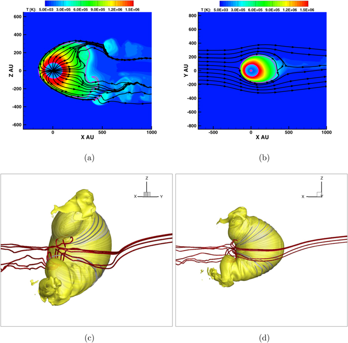
Figure 2. Slice in the meridional plane (a) of the solar velocity streamlines from the SHIELD model. Interstellar velocity streamlines are shown in the equatorial plane in panel (b). Both are shown with contours of the plasma temperature, the magenta line denotes the location where Tp = 4.4 × 10⁵ K. Panel (c) provides a tail view of the heliosphere from the SHIELD model, while panel (d) presents a view from the side. The interstellar streamlines enter the domain from the x = −1500 au face. The HP is defined by the isosurface of Tp = 4.4 × 10⁵ K. The gray lines are the solar magnetic field lines, while the interstellar velocity streamlines are shown in red.
Download figure:
Standard image High-resolution imageThe effect of the kinetic treatment of the neutrals within the SHIELD model is presented in Figures 3–5. It is evident in all of the figures that the two-lobe structure of the heliosphere persists. Figure 3 presents both a view of the port side and the nose of the heliosphere for the multi-fluid model (Figures 3(b) and (a)) as well as for SHIELD (Figures 3(e) and (d)). The HP is defined by an isosurface of Tp = 4.4 × 10⁵ K, shown in yellow. This temperature best captures the solar magnetic field lines that are marked as gray rods inside the isosurface. The interstellar magnetic field lines are shown in red and reconnect in the port side similar to the work of Opher et al. (2017). As is noticeable in Figure 3(a), the draped interstellar field appears to be less affected by reconnection in the SHIELD model, however, the pattern of reconnection and details of true draping depends on the turbulence within the lobes (Opher et al. 2017) and is left for future work.

Figure 3. Nose and side views of the heliosphere are shown for the multi-fluid model (top panels), and for the K-MHD results of the SHIELD model (bottom panels). For the left and middle columns, the HP is defined by the isosurface of Tp = 4.4 × 10⁵ K to capture the last field lines with a footpoint connecting to the Sun. The right panels show the HP defined as an isosurface of number density np = 0.022 cm−3. The gray lines are the solar magnetic field lines, while the interstellar magnetic field lines are red.
Download figure:
Standard image High-resolution imageA comparison of the TS and HP locations in the meridional plane between the two models is presented in Figure 4(a). The TS location is defined when the sonic Mach number of the supersonic solar wind reaches a value of one. The HP is defined by the location of the last solar magnetic field line not open to the ISM. This is marked by a plasma temperature of Tp = 4.4 × 10⁵ K. The SHIELD model is shown in red while the multi-fluid model is shown in blue. The interstellar magnetic field pushes the lobes toward the starboard side of the heliosphere. This causes the heliotail to appear truncated and round in the meridional plane. To show the lobes directly, Figure 4(b) presents the HP location in the starboard side in the y = 150 au plane. As seen by Michael et al. (2020), the kinetic neutral hydrogen affects the heliospheric boundaries in the nose similar to the hydrodynamic run used for verification of the SHIELD model. The kinetic neutrals cause the TS and HP to be located 4 au closer to the Sun in the nose direction. Along the Z direction, containing the rotational axis of the Sun, the heliosphere is smaller in the SHIELD model. This can be seen in both panels of Figure 4. The distance between the HP location in the Northern hemisphere and the Southern hemisphere at the location of the Sun (x = 0) is 54 au and 80 au less than in the multi-fluid model in the meridional and y = 150 au planes, respectively. In the tail, the SHIELD model predicts that the TS is located 10 au further from the Sun than the multi-fluid model. As suggested by Pogorelov et al. (2015) and Izmodenov & Alexashov (2018), the kinetic neutrals do indeed move the stagnation point in the tail, with the HP moving 100 au further from the Sun in the meridional plane. However, the two-lobe structure of the HP remains and does not get removed.
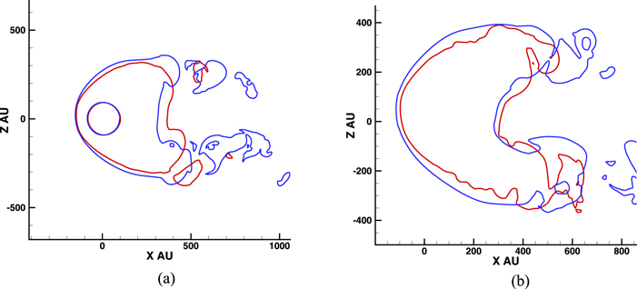
Figure 4. Slices in the meridional plane (a) and y = 150 plane (b) showing the location of the TS and HP, defined as Tp = 4.4 × 10⁵ K, in the multi-fluid model (blue) and the SHIELD model (red). The heliotail is longer in the equatorial plane (Z = 0 au) when the neutrals are solved kinetically but the two-lobe structure still persists.
Download figure:
Standard image High-resolution imageFigure 5 compares the magnetic field strength and plasma speed from the kinetic solution (bottom panels) as well as the multi-fluid approximation (top panels) in the starboard flank. The motion of the TS 10 au farther from the Sun in the SHIELD model results in a magnetic field strength that is 16% lower in the HS down the tail. According to the analytic solution of Drake et al. (2015), a weaker solar wind magnetic field reduces the velocity of the flow within the jets and increases the thickness of the HS. The thicker HS in the SHIELD model can be seen in Figure 4. The fastest speeds in the HS occur near the HP close to the extension of the rotational axes of the Sun. Figure 5(f) shows the speed in this region is reduced in the SHIELD model, confirming a weakening of the collimation of the solar wind with the kinetic treatment of the neutrals. Additionally, in the K-MHD model, the plasma speed in the tail does not decrease as rapidly as the multi-fluid model. The higher speed strengthens the ram pressure of the solar wind, resulting in a tail that is located farther away in the SHIELD model.
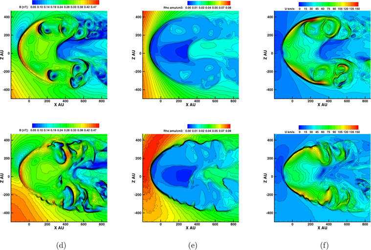
Figure 5. Panels show the magnetic field strength (nT), plasma density (cm−3), and plasma speed (km s−1) in the y = 150 plane for the multi-fluid model of Opher et al. (2015) (top panels) and SHIELD model (bottom panels).
Download figure:
Standard image High-resolution imageThe difference between the SHIELD model results and those of Izmodenov & Alexashov (2018) could also be due to the numerical scheme choice on how to handle the HP within the K-MHD models. Opher et al. (2015) and the SHIELD model allow for reconnection, instabilities, and exchange between the ISM and solar plasma. This numerical reconnection causes the draped ISM to have the same direction as the Parker spiral (Opher et al. 2017) and mixes the solar and ISM plasma in between the lobes, forming a plasma environment with intermediate values compared to solar and ISM values (Michael et al. 2018). The magnetic field within the lobes also becomes unstable in the heliotail, as seen in Figures 3 and 5. This turbulence adds an additional source of mixed ISM and solar plasma. The mixing of ISM and solar plasma is strictly prohibited in the model of Izmodenov & Alexashov (2018), which treats the HP as perfectly ideal, allowing for no communication across the HP. While the specific treatment of the HP is important and impacts the plasma solution, the kinetic treatment of the neutrals is not the cause for the removal of the two-lobe structure and the formation of a long comet-like tail.
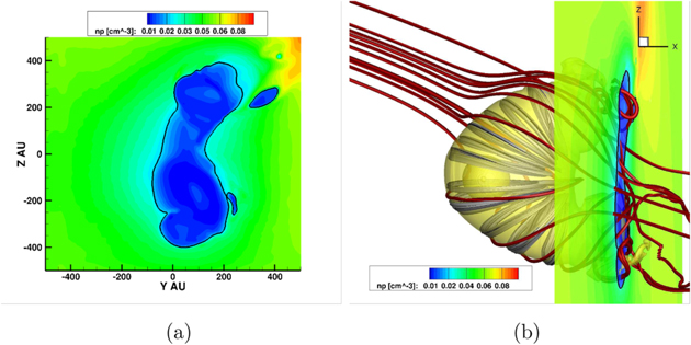
The location of the HP in the SHIELD model is determined during post-processing. In this work, we define the HP by the location of the last solar magnetic field lines. As noted by Michael et al. (2018), if another criteria is used, the heliotail could appear to be long even when the collimation of the solar wind is occurring. When the HP is defined by an intermediate density between the HS and ISM, a long tail forms in both our multi-fluid model, Figure 3(c), and the SHIELD model, Figure 3(f). With this definition of the HP, the solar wind would be collimated by the solar magnetic field yet the HP would appear to remain long and comet-like, as the intermediate, mixed solar and ISM plasma between the lobes seen further down the heliotail reside on field lines open to the ISM, Figure 6. A study is needed to determine whether each model is using the same HP definition. This is important to disentangle the differences between the model results and point to the overall impact of numerical reconnection and heliotail instabilities on the stability of the two-lobe structure of the heliotail.
Figure 6. Plasma density shown in the x = 500 au plane down the tail in the SHIELD model (a). The black line denotes where the plasma density is equal to np = 0.022 cm−3; (b) shows the magnetic field lines that cross the x = 500 au plane in relation to the isosurface of Tp = 4.4 × 10⁵ K.
Download figure:
Standard image High-resolution image
4. Summary and Conclusions
The two-lobe structure persists with a kinetic treatment for the neutrals within the K-MHD solution of the SHIELD model. The kinetic neutral hydrogen weakens the magnetic field strength in the HS. This reduces the collimation force and causing the HP to be located 100 au further down the tail. The HP, defined by the temperature matching the last solar field lines, remains short. This is in contrast to other studies which claimed the kinetic treatment of neutral atoms causes a long, comet-like heliotail. We conclude that this discrepancy could be how the HP is defined within the models or the different numerical treatments of the HP that do and do not allow for numerical reconnection or instabilities to cause the solar and interstellar plasma to mix in between the two lobes.
This work was supported by NASA Headquarters under the NASA Earth and Space Science Fellowship Program: grant NNX14AO14H, and by NASA grant 18-DRIVE18_2-0029, Our Heliospheric Shield, 80NSSC20K0603. A.M. and M.O. acknowledge the support of NASA Grand Challenge NNX14AIB0G and the Hariri fellowship from Boston University. The calculations were performed at NASA AMES on the Pleiades supercomputer.