

Abstract
Undergraduate experiments provide practical demonstration of both measurement techniques and the underpinning science. The radioactive source 44Ti is particularly useful due to the range of experimental measurements it allows. Five experiments utilising 44Ti, suitable for undergraduate laboratories, are described in this paper. These illustrate several topics in nuclear physics and a number of experimental techniques, such as coincidence measurements and lifetime measurements. The experiments described require careful evaluation of the data which provide students with important analytical skills.
Export citation and abstract BibTeX RIS

Original content from this work may be used under the terms of the Creative Commons Attribution 4.0 licence. Any further distribution of this work must maintain attribution to the author(s) and the title of the work, journal citation and DOI.
1. Introduction
Undergraduate laboratories are tasked with developing students' experimental skills as well as teaching new physics and cementing ideas in place that have already been covered in lecture courses. With this in mind, the radioactive isotope 44Ti has much to offer as a teaching laboratory source of radiation. This paper presents an overview of the properties of this source followed by a detailed description of possible experiments and the techniques involved.
The neutron deficient 44Ti decays by electron capture to 44Sc before decaying to the stable isotope 44Ca by predominantly positron emission. The ground state to ground state Q-values for these decays are 268 keV and 3652 keV respectively [1]. This shows the typical behaviour of Q-values for beta decay along a line of even A isobars, which can be linked to the pairing term in the semi-empirical mass formula (SEMF) [2]. Pure electron capture of the 44Ti decay is due to the low Q-value whereas the higher Q-value for the decay of 44Sc allows positron emission to both the ground state and first excited state in 44Ca. However, spin and parity constraints show that the decay to the ground state of 44Ca is doubly forbidden [3]. The first excited state takes 98.97% of the decay strength with 94.27% of the decay proceeding through positron emission. The decay of 44Sc to the second and third excited states of 44Ca is allowed, but as the Q-value is below the β+ threshold these pure electron capture decays are weak. The fourth excited state of 44Ca has Jπ = 3−, hence the electron capture process is first forbidden. The decay energy to this state is only 2% lower than that to the third excited state but the intensity is four times smaller. The decay scheme of 44Ti is summarised in figure 1.
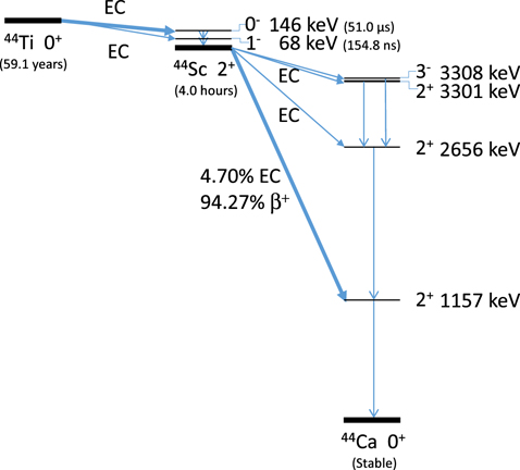
Figure 1. Decay scheme for 44Ti, showing the decay through 44Sc to the ground state of 44Ca.
Download figure:
Standard image High-resolution imageThe decay of the 0+ ground state of 44Ti to the 0− second excited state of 44Sc is a first forbidden Gamow–Teller decay but still takes 99.6% of the decay strength. Decay to the 1− first excited state is also forbidden but could proceed via either the Fermi or Gamow–Teller decay paths. The ground-state to ground-state decay (0+ → 2+) is doubly forbidden and as such makes a negligible contribution. The first and second excited states in 44Sc are isomeric with life-times of 154.8 ns and 51.0 μs seconds respectively [1]. The longevity of these states and the preferred decay paths require a more detailed understanding of the nuclear physics which can be obtained by reference to the Nilsson model diagram for this mass region [4].
Electron capture results in inner shell vacancies in the daughter atom. The atom then relaxes via x-ray emission or the emission of Auger electrons. X-rays are also emitted following internal electron conversion transitions which compete weakly (8% and 3%) [5] with the gamma decay of the first and second excited states in 44Sc respectively.
The experiments described below will investigate the decay sequence from 44Ti via 44Sc to 44Ca, measure the half-lives of the first and second excited states in 44Sc and look at the angular correlation [6] of the 68 and 78 keV γ rays from the decay of excited states in 44Sc. An additional experiment uses the coincidence rate for detecting two gamma rays to determine the absolute activity of the source and the efficiency of the detector.
In addition to the experiments described in this paper the 44Ti source has proved to be a useful general purpose source for detector calibration. The source provides γ ray energies of 68 (I = 93.0%), 78 (I = 96.4%), 511 (I = 188.5%), 1157 (I = 99.4%), 1499 (I = 0.91%), and 2656 (I = 0.11%) keV. Two further calibration points are obtained at 146 and 1668 keV by the simultaneous detection of two γ photons.
The sources used in these experiments were produced by irradiating stacks of scandium foils with a 25 MeV proton beam provided by the Birmingham MC40 cyclotron, utilising the 45Sc(1H,2n)44Ti reaction (Q = −12.3770 ± 0.0010 MeV). Other methods of production are not straightforward, due either to instability of the potential target nucleus, such as 44Sc(1H,n) and 41Ca(4He,n), or lack of natural abundance of the target nucleus, such as 42Ca(3He,n) (42Ca has only a 0.65% abundance). The latter reaction has a cross-section ≈150 mb at 11 MeV, roughly similar to that of the (1H,2n) route at 25 MeV, but also produces radioactive 41Ca as a product ( years), which further decreases the appeal of this production method. Other, more symmetric reactions are possible, but these require higher energies and more complex ion sources. For the 45Sc(1H,2n)44Ti reaction, the cross-section is very low below 24 MeV, so can be produced by cyclotrons with k ⩾ 24 MeV or ⩾12 MV tandem accelerators. A beam intensity of about 10 μA was used over a period of approximately 20 h. A stack of six 0.1 mm foils was irradiated to produce a stronger set of sources (between 9 and 12 kBq), while weaker and thinner sources which are used as open sources (see section 4 for more details) were produced by irradiating four 0.0125 mm thick foils, giving an activity of about 3 kBq.
Several techniques are utilised in the detailed experiments: using coincidence techniques via a timing single channel analyser (TSCA) and gate-and-delay generator (G&DG) to obtain energy spectra from a detector dependent on detection of a photon of specific energy by a second detector; measurement of the half-life of a nuclear state using the signals of two detectors, one measuring the photon that feeds the transition and the other measuring the photon characteristic of the de-excitation of the state, to generate logic pulses, and repeated measurement of the time elapsed between the pulses using a time-to-amplitude converter (TAC); measurement of the half-life of a nuclear state using one detector, detecting both photons in the same detector and delaying one signal by a set amount in order to measure the half-life; and measurement of the angular correlation between two sequential photons, utilising coincidence techniques with two detectors to generate a TAC spectrum at a range of angles.
2. Decay sequence of 44Ti
A 44Ti spectrum, as shown in figures 2 and 4, taken with a hyper-pure germanium (HPGe) detector shows strong lines at 68, 78, 511 and 1157 keV. The summation peaks at 146 keV and 1668 keV are from the simultaneous detection of the 68 and 78 keV and 511 keV and 1157 keV gamma rays respectively. As such, their strength relative to the other lines will be dependent on the solid angle between the source and detector. The weak line at 1499 keV is just above the 1461 keV 40K background line while the 2656 keV line is clearly seen to the right of a stronger background line, the commonly observed 2.6 MeV line from 208Tl. The very weak lines at 2144, 2151 and 3301 keV are all lost in the noise.
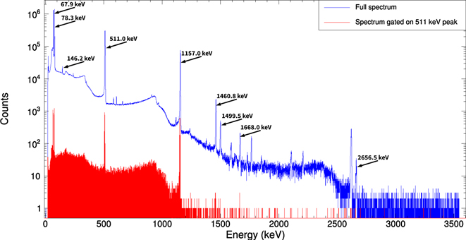
Figure 2. Spectra of 44Ti source measured with a HPGe detector. The blue spectrum was ungated while the red spectrum shows a coincidence spectrum gated by the 511 keV line measured in a second HPGe detector.
Download figure:
Standard image High-resolution imageThe electronics set up, used to determine the decay sequence, is shown in figure 3. The lower detector in figure 3 was used to provide a gate signal to one of the analogue-to-digital converters (ADCs) connected to the upper detector, shown as ADC 1 (configuration B) in figure 3. To set the energy gate of the TSCA for the lower detector, positive logic signals from the TSCA were used to trigger the G&DG. This provided a positive square gate signal into one channel of an oscilloscope. Triggering on this signal, the analogue energy signal in channel two of the oscilloscope was brought into alignment with the gate signal by adjusting the delay on delay amplifier 1 or the delays on the TSCA and G&DG. The gate width was also adjusted to match the width of the energy pulse. The analogue signal was then passed to the input of ADC 1 while the gate signal for ADC 1 was provided by the G&DG. A spectrum was produced without the gate and a region of interest highlighted around the required γ ray energy. For the initial set-up it is best to work with the 511 keV line as this will more easily allow the timing between the two detectors to be synchronised. The gate was then activated and the TSCA window adjusted to select only events in the highlighted region. Having set the TSCA window, ADC 1, shown by the dashed lines in figure 3 in configuration A, was redeployed to configuration B (solid lines).
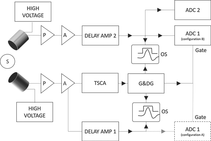
Figure 3. Electronics used to determine the decay sequence. P represents a preamplifier, A represents an amplifier, G&DG represents a gate and delay generator, ADC represents an analogue-to-digital converter, OS represents an oscilloscope and S represents a 44Ti source. The detectors are shown as cylinders. The dashed line represents the electronics set-up required with the ADC in order to set an energy range on the TSCA.
Download figure:
Standard image High-resolution imageUsing the gate signal to trigger the oscilloscope, the analogue signals from the upper detector were brought into time coincidence with the gate signal by adjusting the delay, via delay amplifier 2, in the upper channel. Due to random coincidences this was not as clear as setting the time coincidence using just one detector. However, by placing the source between the two detectors the coincidence rate was enhanced by using the 511 keV annihilation γ rays.
Once the timing had been set up, the source was positioned such that back-to-back annihilation photons could not be simultaneously detected in both detectors. To save time, data were taken with two ADCs (ADC 2 and the redeployed ADC 1). A single ADC can be used but requires sequential gated and ungated experimental runs. ADC 1 was gated by the lower detector while the other was ungated. The gate provided by the lower detector was adjusted to select any of the γ rays emitted from the source.
As shown in figure 2 with the gate signal enabled by the 511 keV γ rays, the counting rates of the 68 and 78 keV lines relative to the 1157 keV line were strongly diminished and their intensities were in line with the count rate for random coincidences during the time the logic gate was open. This indicated that the low energy γ rays were not in coincidence with the positron decay. The 1499 keV line in the gated spectrum was very weak and its relative strength to the 1461 keV line from 40K was similar to that shown in the ungated spectrum. This indicated that it was not in coincidence with the annihilation photons.
Placing a gate on the 1157 keV line, as shown in figure 4, showed it was in coincidence with the annihilation photons but not the 68 and 78 keV γ rays. In the ungated spectrum the 1499 keV line was seen close to the 1461 keV contamination line from 40K. The gated spectrum showed suppression of the contaminant but the weak peak for the 1499 keV transition was clearly visible showing it was in coincidence with the 1157 keV line. In order to see suppression of the 2656 keV line when the 1157 keV transition was used to gate the signal, a very long run time is required. The spectrum shown in figure 4 was taken over a period of 5 h 20 min, but as can be seen in figure 4 the counts acquired at this energy were too few to draw any significant conclusion. This would be typical of the time an undergraduate might have to take data, using a full laboratory session. Longer measurements were possible with overnight runs.
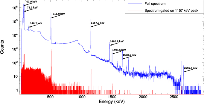
Figure 4. Spectra of 44Ti source taken with a HPGe detector. The blue spectrum was ungated while the red spectrum was gated by the 1157 keV line measured simultaneously in a second HPGe detector.
Download figure:
Standard image High-resolution imageUnable to gain meaningful information about the origin of the 2656 keV line from coincidence measurements, one can infer from the sum of energies 2656 = 1157 + 1499 that the 1157 keV and 1499 keV follow a sequential decay of the 2656 keV level. Given that the 1499 keV transition was not in coincidence with 511 keV annihilation photons, the decay sequence must be as shown in figure 5, although it could not be ascertained whether the first excited state in 44Sc is at 68 or 78 keV until a half-life measurement had been made.
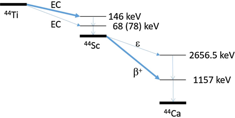
Figure 5. Decay scheme for 44Ti based on analysis in this paper.
Download figure:
Standard image High-resolution imageThe 1157 keV line is populated by positron decay while the higher lying levels are below the Q-value threshold for β+decay and thus decay by the weaker electron capture process. This is often an area where students get confused, due to balancing atomic, rather than bare nuclear masses. This experiment reinforces the Q-value calculation performed by students. The results are consistent with the lowest energy γ rays belonging to the decay of excited states in 44Sc, but at this stage this cannot be proved. Likewise the high Q-value of 1022 keV needed for positron decay would indicate a ground state to ground state Q-value of at least 2179 keV if the decay populates a state at 1157 keV. Based on the pairing term in the SEMF, this would suggest the positron emission is from the 44Sc decay to 44Ca. Further clarification of the decay sequence can be obtained from half-life measurements of the excited states in 44Sc.
3. Half-life of the first excited state in 44Sc
The first excited state of 44Sc is predominantly populated by the 78 keV γ-decay from the second excited state. It is depopulated by the 68 keV γ-decay to the ground state. The half-life can be measured by using two detectors and TSCAs to provide time signals which then are input into a TAC. If one TSCA gate is set on the 78 keV γ ray and the other on the 68 keV γ ray, a characteristic decay curve will be produced. This will be a convolution of an exponential decay curve and a Gaussian function. The Gaussian is a result of the time resolution of the system. The width of the Gaussian can be determined by a coincidence measurement between two prompt γ decays. The half-life of the first excited state can then be determined by fitting the time spectrum with a convolution of the Gaussian and exponential curves. This extends the concept of resolution to timing—something that is frequently glossed over by students who tend to consider only the energy resolution of the detectors. Starting the TAC with the 78 keV γ ray produces an exponential decay curve which falls with increasing time while starting the TAC with the 68 keV, while delaying the associated stop signal, causes the curve to increase with time. This is sufficient information to prove that the first excited state is at 68 keV.
If the TSCAs are gated by both the 68 and 78 keV γ rays and a suitable time delay given to the stop signal, the time spectrum will take the form of a rising exponential followed by a falling exponential. A small dip or rise in the centre, as seen in figure 6, could be due to time walk of the constant fraction TSCA. Alternatively, if an enhancement of the counting rate is only seen at the peak of the time spectrum, when the source lies on a line between the centres of the detectors, the enhancement at the peak could be caused by prompt coincidences between 511 keV annihilation γ rays which have produced Compton continuum events with the same energies as the 68–78 keV lines.
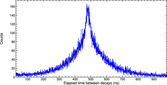
Figure 6. TAC spectrum for measuring the half-life of the first excited state in 44Sc using two NaI(Tl) scintillation detectors.
Download figure:
Standard image High-resolution imageA single, negatively biased detector, in this case a CeBr3 scintillator, as well as a fast discriminator was used to measure the lifetime of the 1− state, but care was taken to correctly match input and output impedances to avoid reflections. A photomultiplier tube (PMT) with a negatively biased cathode allows for DC coupling between the anode and subsequent electronics. Removing the capacitive coupling results in a faster rise time for the anode pulse and consequently an improved time resolution [7]. The discriminator was set to trigger just below the 68 keV signal from the anode signal of the PMT. The nuclear instrumentation module (NIM) signal from the discriminator was split and one branch delayed by a few nanoseconds. The delayed signal was used to start a TAC and the prompt signal was used as a stop pulse. The time sequence of the pulses is shown in figure 7.
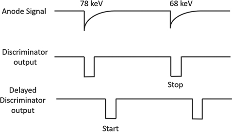
Figure 7. Time sequence of pulses for timing with single detector.
Download figure:
Standard image High-resolution imageAs this method requires both γ rays from the sequential decay to be detected in the same detector, the solid angle needs to be maximised by having the source as close to the detector as possible. As well as this, the dead time needs to be managed (in order to enable detection of both coincident photons) by picking a source of suitable strength, particularly important due to the requirement of solid angle coverage. When collecting the data shown in figure 9, the dead time was kept below 0.5%.
The amplified signals from the last dynode of the PMT were used to provide an energy spectrum. This, in addition to the 68 and 78 keV, showed a sum peak at 146 keV. Logic pulses from a TSCA gating on the 146 keV line provided a coincidence gate for the ADC used to digitise the TAC pulse. This reduced the background distortions in the final time spectrum. However, it should be noted that there will be an energy shortfall for the sum energy if the time between the decay of the second and first excited states is long. Incomplete summation of the charge pulses is due to the lack of alignment between the energy signals entering the ADC. The result is a low energy tail for the sum peak. If working with time ranges of more than 0.5 μs the low energy tail will need to be included when setting the TSCA gate used to gate the TAC spectrum. The electronics are shown in figure 8. Additional electronics, namely a G&DG and DA, similar to those shown in figure 3, were used to set the thresholds for the discriminator and the TSCA energy window.

Figure 8. Electronics for determining the lifetime of the 1− state in 44Sc using a single detector.
Download figure:
Standard image High-resolution imageThe final time spectrum, shown in figure 9, was calibrated by swapping the start and stop signals into the TAC and varying the delay. This provided a time spectrum of delta functions. The time between these was determined by also observing the start and stop pulses on an oscilloscope. The final time spectrum was fitted with a convolution of a Gaussian and an exponential. The TAC calibration is based partly on manufacturer specifications for both the TAC and the oscilloscope. This gave a half-life of 154.2(1) ns and a time resolution, a full width at half maximum, of 9.02(2) ns, where the presented errors are purely statistical. The literature value for this half-life is 154.8(8) ns [1].

Figure 9. TAC spectrum and corresponding fit, a Gaussian and exponential convolution, for data obtained using a single CeBr3 detector. The small bumps that can be seen in the data arise due to small reflections in the electronics. Effort was invested in keeping these to a minimum.
Download figure:
Standard image High-resolution image4. Half-life of the second excited state in 44Sc
The half-life of the 0− state in 44Sc is 51.0(3) μs [1]. It is populated by electron capture, which means the initial population of the state is signalled by the emission of an Auger electron or a characteristic x-ray from 44Sc. The relatively long half-life, and the need to use a ≈4 keV x-ray to signal the populating of the 0− state, place severe constraints on the 44Ti source. The source must be thin enough to allow a significant fraction of the x-rays to escape. Therefore, it is preferable to have an open source but in a teaching environment a thin layer of lacquer applied to the surface will provide protection against contamination for a small loss of signal. The thin sources, described briefly in section 1, were each glued with epoxy resin to a 3 mm thick piece of Perspex. The exposed side of the source was covered with a thin lacquer. Before applying the lacquer to the sources, tests were made by spraying the lacquer onto thin Ti foils and observing the change in attenuation of low energy x-rays, generated by bombarding the foils with 59.5 keV γ rays from 241Am. This allowed the effect of the lacquer on the attenuation to be estimated. Measurements of the ∼4 keV x-rays were made before and after applying the lacquer to the 44Ti source to check that the loss of the x-rays in the lacquer was indeed less than 10%.
In choosing the source activity, a compromise has to be made between the true coincidence rate, the random coincidence rate and the magnitude of correction factors that depend on count rate. Initial calculations suggested an activity of a few kBq would provide a reasonable counting rate without significant background corrections.
A thin beryllium-windowed, Peltier-cooled, Si (PIPS) detector with a 30 mm2 active area was used to detect the 4.086, 4.091 (Kα ) and 4.461 keV (Kβ ) x-rays which have a combined branching ratio of ∼18% for the decay of 44Ti. A TSCA was used to provide a time signal to start a TAC when an x-ray was detected in a gate set around the Kα and Kβ lines. These can be clearly seen in the spectrum shown in figure 10. In addition to the Sc x-rays, the spectrum also shows the Kα line from Ca. The Kβ line from Ca is at 4.013 keV and masked by the Kα line from Sc. The Kα and Kβ lines from Fe are from γ ray fluorescence of the iron in the steel housing of the Si detector.

Figure 10. X-ray spectrum from 44Ti source taken with PIPS detector over 1200 s.
Download figure:
Standard image High-resolution imageThe stop signal for the TAC was provided by a LaCl3(Ce) scintillator and TSCA which was set to register events from both the 68 and 78 keV γ rays from 44Sc. A typical γ-spectrum is shown in figure 11. In addition to the 68 and 78 keV lines from 44Sc there is a peak at 146 keV which is predominantly from the simultaneous detection of the 68 and 78 keV γ rays. Below the 68, 78 and 146 keV lines are the escape peaks from the K x-rays from lanthanum. Also visible in the spectrum are the 511 keV line, from the annihilation of the positrons from the decay of 44Sc, and the 1157 keV line, from 44Ca. These higher energy lines lead to a Compton background under the peaks of interest. The TAC output was fed into an ADC with a 2048 channel multichannel channel buffer. The source was placed between the two detectors with the separation distances kept as small as possible.
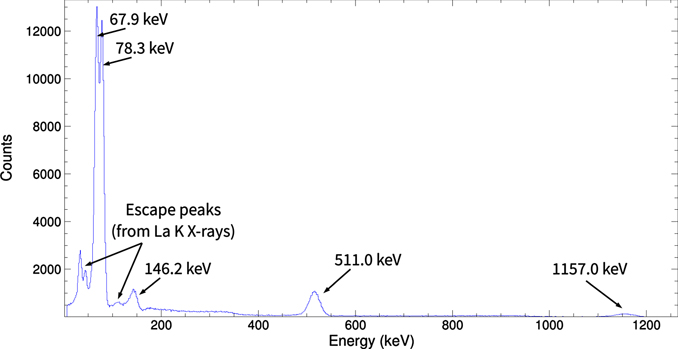
Figure 11. Gamma-ray spectrum for 44Ti measured with a 1' LaCl3(Ce) scintillator detector.
Download figure:
Standard image High-resolution imageBy adjusting the delays on the TSCAs the stop signal was delayed by about 10 μs. A TAC range of 100 μs allowed data to be taken over ≈2 half-lives. The first 200 channels (≈10 μs) proved useful in determining the level of the random coincidences. Once set up, a data taking run of several hours was needed to accumulate enough counts for a statistically significant result to be achieved. Figure 12 shows the time spectrum taken with a 10 μs delay applied to the stop signal. The spectrum shows a constant background from random coincidences in the first 10 μs. The sharp peak after 10 μs is due to coincidences between x-rays from internal electron conversion transitions and γ-decays between the second, first and ground states in 44Sc. Following the sharp peak is the decay curve for the second excited state of 44Sc.
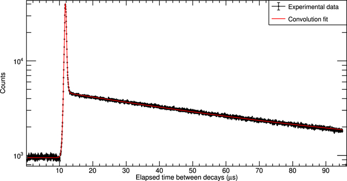
Figure 12. TAC spectrum using x-rays for the start signal and 44Sc γ rays delayed by 10 μs for the stop signal, shown on a logarithmic scale.
Download figure:
Standard image High-resolution imageTo check that the background was constant a run with a 90 μs delay was taken. This showed that within statistical errors the background was constant. The spectrum shown in figure 12 was fit with a constant background and three Gaussian-exponential convolutions detailed below, the first two associated with the 155 ns half-life and the third with the 50 us half-life:
- (a)Starting the TAC by x-rays from internal conversion of the 78.3 keV transition and stopping the TAC with a 67.9 keV photon;
- (b)Starting the TAC by x-rays from internal conversion of the 67.9 keV transition and stopping the TAC with a 78.3 keV photon;
- (c)Starting the TAC by x-rays following electron capture decay of 44Ti and stopping the TAC with either 78.3 keV or 67.9 keV photons.
The half-life obtained for this fit was 41.9(1.5) μs when taking into account systematic effects. This is similar to the published half-life of the second excited state [1], though beyond two standard deviations due to use of an improved experimental set-up with modern detectors and optimised 44Ti source which reduced the random background rate leading to a higher accuracy measurement. Details on the physics significance of this result can be found in reference [8]. This is a great showcase that relevant contemporary measurements can be made in a teaching laboratory.
5. Angular correlations
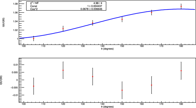
The 0− second excited state of 44Sc decays to the 1− first excited state by an M1 transition and the 1− state decays via an E1 transition to the 2+ ground state. This should give rise to an angular correlation [4] between the two γ rays of the form

where θ is the angular separation of the two γ rays. The coefficient in front of the cos2 θ term can be determined by measuring the angular correlation. Two 2'' NaI(Tl) detectors mounted on rotatable arms of a turntable were used to measure the angular correlation. The detectors were mounted 8 cm from the source. This distance provided a compromise between count rate and angular resolution. The 44Ti source was fixed to a rotatable mount to enable it to be positioned to minimise the attenuation in the source as the detectors are moved to different positions. The signals from the detectors were amplified and a TSCA used to provide NIM signals to a TAC when signals from the 68 and 78 keV γ rays were detected. The logic signals from one of the detectors were used to start the TAC while the signals from the other were delayed by ≈500 ns and used as stop pulses. With a TAC range of 1 μs the time spectrum, in figure 6, shows a combination of a 154 ns rising exponential and a 154 ns falling exponential. Summing the counts in a fixed time window allows the coincidence rate to be calculated as a function of the angle between the two γ rays. Care needs to be taken to avoid counting prompt coincidences from annihilation photons so the window should not include the region around the central area of the peak in the time spectrum. The angular correlation shown in figure 13 shows a plot of I(θ)/I(90) as a function of θ. This was fitted with the function f(θ) = a + b cos2 θ + c cos4 θ, with best fit parameters a = 1.000 ± 0.005, b = 0.068 ± 0.011 and c = −0.0005 ± 0.0007. The coefficient c of the cos4 θ term is zero within errors which is in agreement with theory. Having found c to be compatible with zero and a = 1.000 ± 0.005, the fitting function was changed to f(θ) = 1 + b cos2 θ. This reduced the uncertainty on the parameters. The final asymmetry for the data obtained was b = 0.068 ± 0.007 which, considering the large angle subtended by the detectors, compares well with the expected value of b = 0.077(=1/13).
Figure 13. Angular correlation between the 78 and 68 keV γ rays from the decay sequence in 44Sc. The blue line shown is a fit to the data points using the function f(θ) = a + b cos2 θ.
Download figure:
Standard image High-resolution image
6. Absolute activity of the source
Titanium-44 decays to 44Sc with a half-life of ∼60 years. The 44Sc half-life is ∼4 h and after a few days the activity of the 44Sc will be determined by that of the parent 44Ti. The absolute activity of the source can be determined by measuring the counting rate, R1, for the 511 keV annihilation photons, R2 for the 1157 keV γ rays and R12 in the 1668 keV peak which records the coincident detection of 511 keV and 1157 keV photons.
The counting rate  depends on the activity, A, of the source, the intrinsic efficiency,
  i
, of the detector, the solid angle, Ωi
, and the radiation intensity, γi
, for the detected photon and the counting rate, Rij
, for detecting two photons simultaneously in the same detector, given by
i
, of the detector, the solid angle, Ωi
, and the radiation intensity, γi
, for the detected photon and the counting rate, Rij
, for detecting two photons simultaneously in the same detector, given by  . If the coincidence rate is small compared to the singles rate, the approximation
  can be made. It is therefore easy to determine the activity of the source by measuring the rates for detecting two photons independently and in coincidence. The activity is then given by A ≃ R1
R2/R12. Although this can be done using two detectors, it is easier to simply look for the individual γ ray full energy peaks and the sum peak in a single detector.
can be made. It is therefore easy to determine the activity of the source by measuring the rates for detecting two photons independently and in coincidence. The activity is then given by A ≃ R1
R2/R12. Although this can be done using two detectors, it is easier to simply look for the individual γ ray full energy peaks and the sum peak in a single detector.
7. Discussion
The experiments described in this work were all offered, along with a selection of other experiments, to third year undergraduate students. The students, working in pairs, took four afternoons to understand their equipment by producing energy calibrations, efficiency and resolution measurements as functions of energy for their detectors, before embarking on one of the experiments described. Each project described was completed over a 2 week period with 16 h of laboratory time allocated. Dissemination of the information obtained by each pair of students to the class as a whole was made via 10 min presentations by each pair of students in a final laboratory session. The experiments were designed to show a variety of techniques using different types of radiation detectors and a variety of nuclear instrumentation module (NIM) based electronics modules. Through the seminars, a comparison of detector efficiency and resolution could be made for hyper-pure germanium detectors and a range of scintillators which included NaI(Tl), CeBr3, LaBr3(Ce), and LaCl3(Ce). The advantages of using negative bias for the PMTs could be seen in the time resolution of the detectors. The importance of background subtraction and gaining statistically significant data are evident in all of these experiments. With the gated spectra the effect of gate width on the random coincidence rate was also investigated with a critical appraisal of the experimental methods used. Atomic x-ray interactions were observed directly with the PIPS detector and indirectly as escape peaks associated with the detection of low energy γ rays.
The nuclear physics covered topics such as β−, β+ decay and electron capture which had already been taught at undergraduate level. The intensities of the decay channels and half-lives were linked to selection rules, but where there were apparent discrepancies the topic of shape isomerism was introduced to the students. The nuclear physics also covered Q-values along a short length of an even isobar chain of isotopes, competition between γ decay and internal conversion and angular correlations.
8. Conclusion
The long lifetime of the source (59.1 years) as well as the interesting decay scheme makes 44Ti ideal for undergraduate teaching laboratories, enabling lots of interesting experiments which introduce students to many nuclear physics concepts and also provide experience operating nuclear electronics. The decay of 44Ti emits a range of photons in a usable range, from 4 keV to 2656 keV, which further allows the source to be an excellent general purpose source for undergraduate teaching laboratories. The experiments described in this paper provide reinforcement of some ideas taught in nuclear physics lectures as well as extending that material. The experiments also develop students' laboratory skills and data analysis techniques. The common theme of understanding the nuclear physics of a single decay chain fosters an interest in what the group as a whole achieved.