A Novel Global Sensitivity Measure Based on Probability Weighted Moments

Abstract

Global sensitivity analysis (GSA) is a useful tool to evaluate the influence of input variables in the whole distribution range. Variance-based methods and moment-independent methods are widely studied and popular GSA techniques despite their several shortcomings. Since probability weighted moments (PWMs) include more information than classical moments and can be accurately estimated from small samples, a novel global sensitivity measure based on PWMs is proposed. Then, two methods are introduced to estimate the proposed measure, i.e., double-loop-repeated-set numerical estimation and double-loop-single-set numerical estimation. Several numerical and engineering examples are used to show its advantages.

1. Introduction

The purpose of sensitivity analysis (SA) is to determine which of the inputs play more significant roles in reducing the uncertainty in the model output. It is useful because it can rank variables, simplify models, establish priorities for research, and so on [1]. Generally, according to different analysis purposes, the available SA techniques can be classified into local SA (LSA) and global SA (GSA). GSA is a more widely used sensitivity analysis method because it does not rely on the choice of a nominal point and the information of the full distribution range is investigated.

In the past few decades, many GSA methods have been studied. Among them, two categories of methods are widely studied and employed: variance-based global sensitivity measures and moment-independent global sensitivity measures.

Variance-based global sensitivity measures, which are usually called Sobol’ indices, were proposed and developed by Sobol’ [2], Iman [3], Homma [4], and Saltelli [5]. Besides, there are several mature techniques available to solve the above indices, for instance, Monte Carlo simulation, quasi-Monte Carlo simulation, high-dimensional model representation (HDMR), Markovian integration [6], and the surrogate-assisted method [7,8]. Variance-based global sensitivity measures have been widely applied in various fields such as the spray-drying process [9], heap leaching [10], the rainfall-runoff model [11], and polymeric material [12]. However, the variance is not fully representative of uncertainty, especially in some problems where higher moments have more of an effect. Cox [13] and Huber [14] pointed out that “mean-variance decision-making violates the principle that a rational decisionmaker should prefer higher to lower probabilities of receiving a fixed gain, all else being equal”.

To include the whole information of output distribution, moment-independent global sensitivity measures were proposed [15]. In this regard, Chun’s method preliminarily needs some assumptions [15]. Although the relative entropy-based method can show a ranking of relative importance, the value does not have an absolute physical meaning [16]. Additionally, the delta index introduced by Borgonovo is the most popularly used among them [17]. Cui [18] extended the delta index to the failure probability to deal with reliability models. However, these methods have a relatively large computational cost due to the estimation of probability density functions.

There are other alternative GSA measures. Derivative-based global sensitivity measures were introduced by Kucherenko et al. [19], which can serve as an upper bound on the Sobol’ total sensitivity index [20]. Fort et al. proposed goal-oriented sensitivity indices, which depend on the quantity of interest [21]. Kala proposed new quantile-oriented sensitivity indices based on measuring the distance between a quantile and the average value of the model output [22]. Baroni et al. presented an effective strategy for combining variance- and distribution-based global sensitivity analysis [23].

In this paper, we introduce a novel sensitivity measure based on probability weighted moments (PWMs). PWMs are popular in many science and engineering areas [24]. PWMs are usually used to estimate parameters of a distribution. In contrast with classical moments, high-order PWMs can be accurately estimated from small samples. In addition, PWMs are fairly insensitive to outliers because they are linear combinations of samples [25]. They can serve as constraints of the maximum entropy method to describe the distribution feature of the output, which are similar to classical moments [26]. So, PWMs can reflect the influence of uncertainty and be applied in GSA as well.

The paper continues with a review of dominating global sensitivity measure systems in Section 2. Section 3 provides a brief introduction of probability weighted moments and their applications. Section 4 proposes a new global sensitivity measure based on probability weighted moments. Section 5 develops two numerical estimation methods, i.e., double-loop-repeated-set Quasi Monte Carlo (QMC) and double-loop-single-set QMC, for numerically estimating the presented measure. Section 6 provides three numerical examples and one engineering example. Finally, conclusions are provided.

2. Review of Dominating Global Sensitivity Measure Systems

Consider the computational model under investigation, which is represented by Y = g(X), where Y is the model output of interest and $\mathit{X}=\left(X_1,X_2,\dots ,X_n\right)$ is the n-dimensional vector of the model input.

2.1. Variance-Based Global Sensitivity Measures

By the probabilistic approach, the first-order Sobol’ indices (named the Sobol’ main indices) can be defined as:

$$S_i=\frac{Va{r}_{X_i}\left[E_{{\mathit{X}}_{~i}}\left(Y|X_i\right)\right]}{Var\left(Y\right)}=\frac{Var\left(Y\right)-E_{X_i}\left[Va{r}_{{\mathit{X}}_{~i}}\left(Y|X_i\right)\right]}{Var\left(Y\right)},$$

(1)

whereas the Sobol’ total indices are defined as:

$$S_{Ti}^{}=\frac{E_{{\mathit{X}}_{~i}}\left[Va{r}_{X_i}\left(Y|{\mathit{X}}_{~i}\right)\right]}{Var\left(Y\right)},$$

(2)

where ${\mathit{X}}_{~i}$ means all factors except $X_i$. The main index of $X_i$ represents the degree of uncertainty of the variability of the output response when the variable $X_i$ acts alone. The total index represents the total degree of the influence of $X_i$ on the output response variance, including the interaction of $X_i$ with all other variables. Variance-based importance measures have been widely applied due to model independence, incorporating the effect from the full range of variation of each input factor and reflecting the influence of each input and interaction among inputs as well as the capacity to tackle groups of input factors.

However, variance-based indices are not sufficient to describe output variability when the model output has a highly skewed or fat-tailed distribution [27] because the variance of the output cannot be considered as fully representative of its statistical characteristics. Despite many advantages, such measures show some inevitable limitations.

2.2. Moment-Independent Global Sensitivity Measures

The delta index proposed by Borgonovo, which is based on the probability density function (PDF) of the model output, is applied most extensively [17]:

$${\delta }_i=E_{X_i}[s(X_i)]=\frac{1}{2}{\displaystyle {\int }_{-\infty }^{+\infty }\left[{\displaystyle {\int }_{-\infty }^{+\infty }\left|f_Y(y)-f_{Y|X_i}(y)\right|}dy\right]f_{X_i}(x_i)}d{x}_i,$$

(3)

where $f_Y(y)$ is the unconditional PDF and $f_{Y\left|X_i\right.}(y)$ is the conditional PDF of output $Y$. $f_{Y\left|X_i\right.}(y)$ can be obtained by fixing the input variable $X_i$ at a realization value.

Similarly, the moment-independent global sensitivity measure ${\delta }_{i_1,i_2,\dots ,i_r}$ of a group of inputs $X_{i_1},X_{i_2},\dots ,X_{i_r}$ is defined as follows:

$${\delta }_{i_1,i_2,\dots ,i_r}=\frac{1}{2}{\displaystyle \int \left[{\displaystyle \int \left|f_Y\left(y\right)-f_{Y\left|X_{i_1},X_{i_2},\dots ,X_{i_r}\right.}\left(y\right)\right|dy}\right]f_{X_{i_1},X_{i_2},\dots ,X_{i_r}}(x_{i_1},x_{i_2},\dots ,x_{i_r})d{x}_{i_1}{x}_{i_2},\dots ,x_{i_r}},$$

(4)

where $1\le i_1<i_2<\dots <i_r\le n$, $1\le r\le n$, and $f_{X_{i_1},X_{i_2},\dots ,X_{i_r}}(x_{i_1},x_{i_2},\dots ,x_{i_r})$ is the joint PDF of $X_{i_1},X_{i_2},\dots ,X_{i_r}$.

The delta index is also a global, quantitative, and model-free measure. Its moment-independent property is more important. However, the delta index focuses on estimating only one single effect, and separating main, total effect and interactions are not targeted [23].

3. Probability Weighted Moments

The PWM of a random variable was formally defined by Greenwood et al. [24] as:

$$M_{r,s,t}=E\left[X^r{F}^s{\left(1-F\right)}^t\right]={\displaystyle {\int }_0^1{\left[x\left(F\right)\right]}^r{F}^s{\left(1-F\right)}^{t}dF},$$

(5)

where $r,s,t$ are real numbers; $F$ denotes the cumulative distribution function (CDF); and $x\left(F\right)$ is the inverse of the CDF (also called the quantile function). The two following forms of PWMs are commonly used:

Type 1:

$${\alpha }_k=M_{1,0,k}={\displaystyle {\int }_0^1\left[x\left(F\right)\right]{\left(1-F\right)}^{k}dF}$$

(6)

and

Type 2:

$${\beta }_k=M_{1,k,0}={\displaystyle {\int }_0^1\left[x\left(F\right)\right]F^{k}dF}.$$

(7)

Because these two forms can be converted to each other, we only consider Type 2 PWMs in the following equation. From an ordered random sample of size N, $x_1\le x_2\le \cdots \le x_N$, unbiased estimates ${\widehat{\beta }}_k$ of ${\beta }_k$ can be obtained as [26]:

$${\widehat{\beta }}_k=\frac{1}{N}{\displaystyle \sum _{i=1}^N\left[\left(\begin{array}{c}i-1\\ k\end{array}\right)\right]x_i}/\left(\frac{N-1}{k}\right),$$

(8)

where $k=0,1,\dots ,\left(N-1\right)$ are non-negative integers and the binomial coefficient is given as:

$$\left(\begin{array}{c}n\\ r\end{array}\right)=\frac{n!}{r!\left(n-r\right)!},\hspace{1em}n\ge r\ge 0;\hspace{1em}\mathrm{others}0$$

(9)

.

Equation (7) can also be written as:

$${\beta }_k={\displaystyle {\int }_{-\infty }^{+\infty }xF{\left(x\right)}^{k}f\left(x\right)dx}.$$

(10)

From Equation (10), the PWM can be computed by multiplying each observed element by a weight coefficient that is proportional to its probability. Hence, probability weighted moments usually contain more information than classical moments. When comparing a first-order PWM with a first-order classical moment, the magnitudes of the observed elements of the former are adjusted according to probabilities before calculating the average value [28]. A PWM is more robust because of the insensitivity to outliers and the required sample size is smaller.

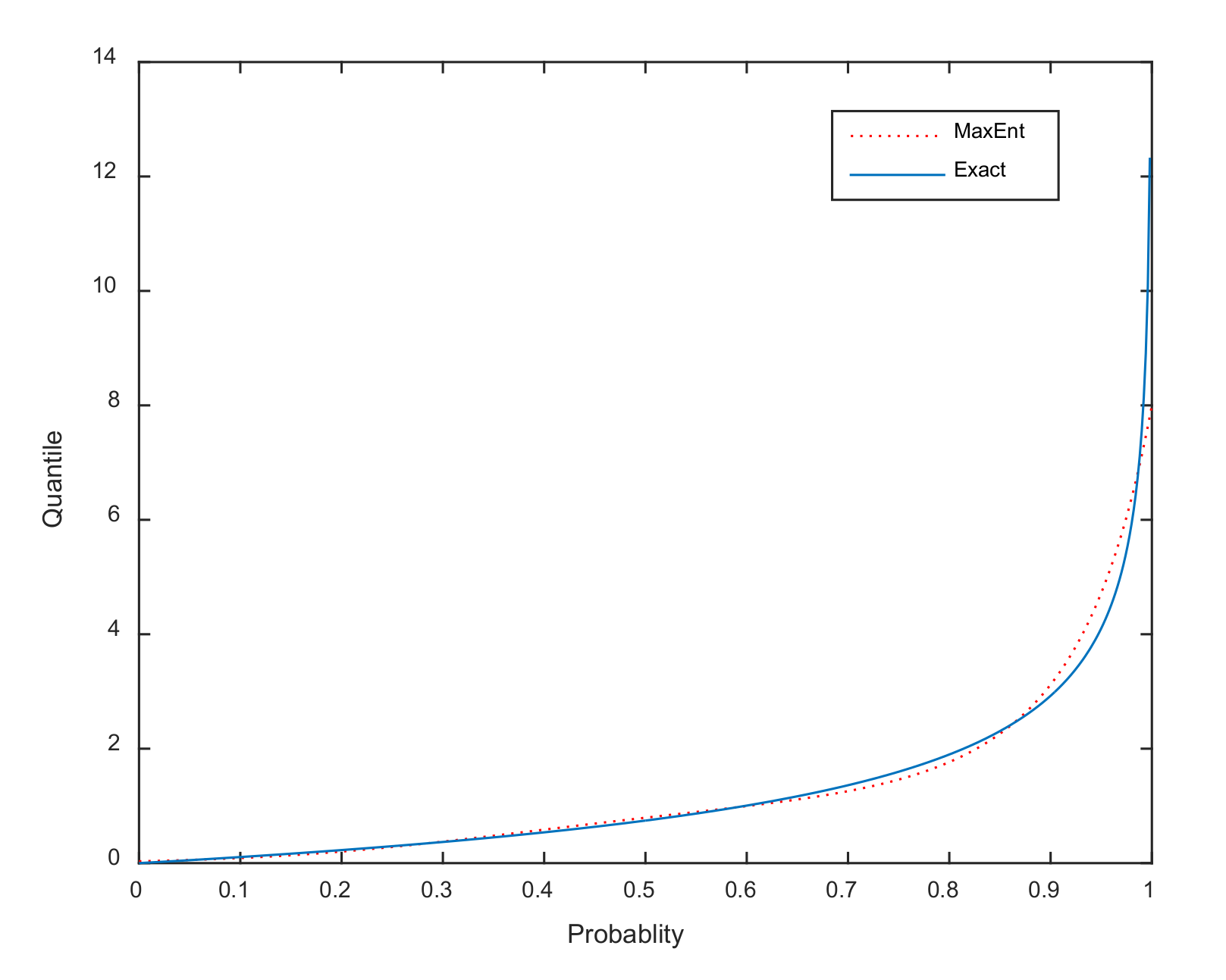
For a non-negative random variable, ${\beta }_k$ can be interpreted as moments of the inverse of the CDF [26]. So, they can serve as constraints in the maximum entropy (MaxEnt) or the minimization cross-entropy [25] approach to estimate the inverse of the CDF. Generally, the estimation using the first four moments often produces an acceptable description. Taking the generalized Pareto distribution (GPD) as an example, its CDF and the inverse of the CDF are given in Appendix A. In the case of $c=-0.2$ and $d=1$, the MaxEnt approximation combined with the first fourth-order PWMs of the Pareto quantile function is shown in Figure 1.

4. Global Sensitivity Measure Based on Probability Weighted Moments

As stated above, not only does a probability weighted moment contain more information than conventional moments, but also it can be accurately estimated from small samples. So, we propose a new global sensitivity measure based on PWMs. It is defined as:

$${\omega }_i^k=\frac{{\beta }_Y^k\left(Y\right)-E_{X_i}\left[{\beta }_{{\mathit{X}}_{~i}}^k\left(Y\left|X_i\right.\right)\right]}{{\beta }_Y^k\left(Y\right)}=1-\frac{E_{X_i}\left[{\beta }_{{\mathit{X}}_{~i}}^k\left(Y\left|X_i\right.\right)\right]}{{\beta }_Y^k\left(Y\right)},\hspace{1em}$$

(11)

where k denotes the order of the PWMs, and the maximal order is usually chosen as 4. Conditional PWMs ${\beta }_{{\mathit{X}}_{~i}}^k\left(Y\left|X_i\right.\right)$ are computed with $X_i$ at a fixed value and ${\mathit{X}}_{~i}$ over their full ranges. $E_{X_i}\left[{\beta }_{{\mathit{X}}_{~i}}^k\left(Y\left|X_i\right.\right)\right]$ is calculated over all possible $X_i$, since $X_i$ is uncertain and its true value is unknown.

To scale the above-mentioned importance measure within the interval [0,1], the final form of the measure based on PWMs can be constructed:

$${\eta }_i^k=\frac{{\left({\omega }_i^k\right)}^2}{{\displaystyle \sum _{j=1}^n{\left({\omega }_j^k\right)}^2}},$$

(12)

where n is the number of input variables.

The numerator ${\beta }_Y^k\left(Y\right)-E_{X_i}\left[{\beta }_{{\mathit{X}}_{~i}}^k\left(Y\left|X_i\right.\right)\right]$ in Equation (11) can be explained as the difference between the original PWM and the average of conditional PWMs. When the contribution of uncertainty from X_i to the difference is bigger, the main measure is bigger as well. Then, we can establish the following properties of the novel global sensitivity measure:

Property 1.

$0\le {\eta }_i^k\le 1$.

Property 2.

${\eta }_i^k=0$means the input variable X_i has no effect on the output.

Proof. 

When the computational model does not include X_i, the conditional distribution $Y\left|X_i\right.$ is equivalent to the distribution of $Y$. It is obvious that $E_{X_i}\left[{\beta }_{{\mathit{X}}_{~i}}^k\left(Y\left|X_i\right.\right)\right]$ is also equivalent to the corresponding ${\beta }_Y^k\left(Y\right)$. So, Equation (11) is equal to 0 and ${\eta }_i^k=0$. □

Property 3.

${\eta }_i^k=1$denotes that only input X_i affects the output.

Proof. 

According to property 2, ${\omega }_i^k$ of all variables except $X_i$ is separately equal to 0. So, we can obtain ${\eta }_i^k=1$ by introducing the values of other variables into Equation (12). □

5. Numerical Estimation for Global Sensitivity Measures

Two numerical methods for estimating ${\eta }_i^k$ indices are proposed in this section. Double-loop-repeated-set numerical estimators are presented in Section 5.1 and double-loop-single-set numerical estimators are presented in Section 5.2.

5.1. Double-Loop-Repeated-Set Numerical Estimators

The most direct method of estimating presented measures is to use the double-loop numerical estimation method. Equations (8) and (9) show the estimator of PWMs, so the key issue is how to estimate conditional PWMs. The main procedures are summarized as follows:

Step 1: Generate N₁ samples of the variable vector $\mathit{x}=\left(x_1,x_2,\dots ,x_n\right)$ by the joint PDF $f_{\mathit{X}}\left(x\right)$ and calculate the corresponding responses $Y$ as well as its kth-order PWM. These samples can be generated by Monte Carlo sampling, Latin hypercube sampling, quasi-Monte Carlo simulation with sampling based on Sobol’ sequences [29,30], or other sampling techniques. Here, quasi-Monte Carlo simulation is recommended for higher and faster convergence.

Step 2: Generate N₂ samples of the input variable X_i by its PDF $f_{{\mathit{X}}_i}\left(x_i\right)$ and denote these samples as $\left(x_{i_1},x_{i_2},\dots ,x_{i_{N_2}}\right)$.

Step 3: The variable X_i should be fixed at $x_{i_m}\left(m=1,\hspace{1em}2,\hspace{1em}\dots N_2\right)$ individually and generate N₃ samples of the remaining variables according to the joint PDF ${\displaystyle \prod _{j\ne i}^n{f}_{{\mathit{X}}_j}\left(x_j\right)}$ (all variables are independent in this paper). So, the conditional PWM of responses ${\beta }_{{\mathit{X}}_{~i}}^k\left(Y\left|X_i=x_{i_m}\right.\right)$ can be obtained, and this step needs to be repeated N₂ times.

Step 4: Calculate the expectation of all conditional PWMs, i.e., $E_{X_i}\left[{\beta }_{{\mathit{X}}_{~i}}^k\left(Y\left|X_i\right.\right)\right]$, and ${\omega }_i^k$ can be easily obtained using Equation (11). After finishing the calculation of ${\omega }_i^k$ of all variables, the normalized versions also can be evaluated in Equation (12).

Step 5: Repeat Step 1–Step 4 under different orders of PWMs. As mentioned in Section 3, we usually let k = 1, 2, 3, and 4.

However, for estimating the presented measure of each individual input, the total number of sampled points is N₁ + n × (N₂ + N₂ × N₃). We denote it as double-loop-repeated-set QMC (DLRS QMC) because this method needs repeated sampling of inputs and outputs in each inner loop. It is obvious that the computational cost would be too heavy.

5.2. Double-Loop-Single-Set Numerical Estimators

We introduce another double-loop QMC method that needs only one set of samples of inputs and outputs for computing presented measures, which is denoted as double-loop-single-set QMC (DLSS QMC).

Step 1: Generate 2 × N₁ samples of whole variables by the joint PDF $f_{\mathit{X}}\left(x\right)$ and assign half of these samples to a sample matrix A:

$$A=\left(\begin{array}{cccc}{x}_1^{\left(1\right)}& x_2^{\left(1\right)}& \cdots & x_n^{\left(1\right)}\\ x_1^{\left(2\right)}& x_2^{\left(2\right)}& \cdots & x_n^{\left(2\right)}\\ ⋮& ⋮& \ddots & ⋮\\ x_1^{\left(N\right)}& x_2^{\left(N\right)}& \cdots & x_n^{\left(N\right)}\end{array}\right)=\left(\begin{array}{c}{\mathit{X}}^1\\ {\mathit{X}}^2\\ ⋮\\ {\mathit{X}}^N\end{array}\right).$$

(13)

Calculate the corresponding responses and estimate the kth-order PWM of $Y$.

Step 2: Matrix B is generated by the remaining samples, which is:

$$\mathit{B}=\left(\begin{array}{cccc}{x}_1^{\left(N+1\right)}& x_2^{\left(N+1\right)}& \cdots & x_n^{\left(N+1\right)}\\ x_1^{\left(N+2\right)}& x_2^{\left(N+2\right)}& \cdots & x_n^{\left(N+2\right)}\\ ⋮& ⋮& \ddots & ⋮\\ x_1^{\left(2N\right)}& x_2^{\left(2N\right)}& \cdots & x_n^{\left(2N\right)}\end{array}\right)=\left(\begin{array}{c}{\mathit{X}}^{N+1}\\ {\mathit{X}}^{N+2}\\ ⋮\\ {\mathit{X}}^{2N}\end{array}\right).$$

(14)

Then, generate a new sample matrix ${\mathit{B}}_A^{\left(p,i\right)}$ by assigning the (p,i)th component of A to the ith column of B:

$${\mathit{B}}_A^{\left(p,i\right)}=\left(\begin{array}{cccc}{x}_1^{\left(N+1\right)}& x_2^{\left(N+1\right)}& \cdots & x_{i-1}^{\left(N+1\right)}\\ x_1^{\left(N+2\right)}& x_2^{\left(N+2\right)}& \cdots & x_{i-1}^{\left(2\right)}\\ ⋮& ⋮& \ddots & ⋮\\ x_1^{\left(2N\right)}& x_2^{\left(2N\right)}& \cdots & x_{i-1}^{\left(2N\right)}\end{array}\hspace{1em}\hspace{1em}\begin{array}{cccc}{x}_i^{\left(p\right)}& x_{i+1}^{\left(N+1\right)}& \cdots & x_n^{\left(N+1\right)}\\ x_i^{\left(p\right)}& x_{i+1}^{\left(N+2\right)}& \cdots & x_n^{\left(N+2\right)}\\ ⋮& ⋮& \ddots & ⋮\\ x_i^{\left(p\right)}& x_{i+1}^{\left(2N\right)}& \cdots & x_n^{\left(2N\right)}\end{array}\right).$$

(15)

Step 3: Calculate the conditional PWM of responses ${\beta }_{{\mathit{X}}_{~i}}^k\left(Y\left|X_i=x_{i_m}\right.\right)$, which is based on the sample matrix $B_A^{\left(p,i\right)}$.

Steps 4 and 5 are identical to those for DLRS QMC.

The total number of sampled points is only (2 + n) × N₁, contributing to a large reduction in sampling time compared to DLRS QMC. N₁, N₂, and N₃ are in the same order of magnitude, which is not more than 4000 usually. Hence, to reduce the calculation cost, the following examples are all solved by the DLSS QMC method.

6. Examples and Discussion

6.1. Numerical Example 1: Linear Function with Normal Distribution Variables

Consider the linear function:

$$Y=a_1{X}_1+a_2{X}_2+\cdots +a_n{X}_n,$$

(16)

where $x_i\left(i=1,2,\cdots ,n\right)$ are independent and normally distributed, i.e., $X_i~N\left({\mu }_i,{\sigma }_i^2\right)$. It is easy to calculate the values of Sobol’ indices, which are:

$$.S_i=S_{T_i}=\frac{a_i^2{\sigma }_i^2}{{\displaystyle \sum _{j=1}^n{a}_j^2{\sigma }_j^2}}$$

(17)

The PDF of the model response is also a normally distributed variable, $Y~N\left({\displaystyle \sum _{i=1}^n{a}_i}{\mu }_i,{\displaystyle \sum _{i=1}^n{a}_i^2}{\sigma }_i^2\right)$, and the conditional response $Y\left|X_i\right.$ is also normally distributed, $Y\left|X_i\right.~N\left(a_i{X}_i+{\displaystyle \sum _{j=1,j\ne i}^n{a}_j}{\mu }_j,{\displaystyle \sum _{j=1,j\ne i}^n{a}_j^2}{\sigma }_j^2\right)$. So, we can obtain the analytical expression of the components of presented measures in such a situation:

$${\beta }_Y^k\left(Y\right)={\displaystyle {\int }_0^1\left({\displaystyle \sum _{i=1}^n{a}_i}{\mu }_i+{\mathsf{\Phi }}^{-1}\left(F\right)\sqrt{{\displaystyle \sum _{i=1}^n{a}_i^2}{\sigma }_i^2}\right)F^k}dF,$$

(18)

$$E_{X_i}\left[{\beta }_{{\mathit{X}}_{~i}}^k\left(Y\left|X_i\right.\right)\right]={\displaystyle {\int }_{R^1}^{}{\displaystyle {\int }_0^1\left(a_i{x}_i+{\displaystyle \sum _{j=1,j\ne i}^n{a}_j}{\mu }_j+{\mathsf{\Phi }}^{-1}\left(F\right)\sqrt{{\displaystyle \sum _{j=1,j\ne i}^n{a}_j^2}{\sigma }_j^2}\right)F^k{f}_{X_i}(x_i)}dF}d{x}_i,$$

(19)

where ${\mathsf{\Phi }}^{-1}$ denotes the inverse of the CDF of the standard normal distribution.

Table 1. Different cases of Example 1.

	Same Value of All Variables	Different Values of All Variables	Parameters
Case 1	${\mu }_i$,${\sigma }_i$,$\left|a_i\right|$	/	$\mu =\left[5,5,5,5\right]$, $\sigma =\left[1,1,1,1\right]$, $\mathit{a}=\left[1,-1,1,-1\right]$
Case 2	${\mu }_i$,${\sigma }_i$,	$\left|a_i\right|$	$\mu =\left[5,5,5,5\right]$, $\sigma =\left[1,1,1,1\right]$, $\mathit{a}=\left[1,2,3,4\right]$
Case 3	$a_i$,${\sigma }_i$,$\left|{\mu }_i\right|$	/	$\mu =\left[5,-5,5,-5\right]$, $\sigma =\left[1,1,1,1\right]$, $\mathit{a}=\left[1,1,1,1\right]$
Case 4	$a_i$,${\sigma }_i$	$\left|{\mu }_i\right|$	$\mu =\left[3,5,7,9\right]$, $\sigma =\left[1,1,1,1\right]$, $\mathit{a}=\left[1,1,1,1\right]$
Case 5	$a_i$,${\mu }_i$	${\sigma }_i$	$\mu =\left[5,5,5,5\right]$, $\sigma =\left[0.5,1,1.5,2\right]$, $\mathit{a}=\left[1,1,1,1\right]$

Note: For all cases, i = 1, 2, 3, and 4.

lists several representative cases and corresponding examples in detail. Then, three importance measures, i.e., Sobol’ indices, delta moment-independent indices, and measures based on PWMs, are calculated, as shown in

Table 2. Results of three importance measures.

Measures	Si (STi)	${\mathit{\delta }}_{\mathit{i}}$	${\mathit{\eta }}_{\mathit{i}}^{\mathit{k}}$
Case 1	[0.2500, 0.2500, 0.2500, 0.2500]	[0.1808, 0.1808, 0.1808, 0.1808]	[0.2500, 0.2500, 0.2500, 0.2500]
Case 2	[0.0333, 0.1333, 0.3000, 0.5334]	[0.0567, 0.1231, 0.2041, 0.3182]	[0.0021, 0.0361, 0.2019, 0.7599]
Case 3	[0.2500, 0.2500, 0.2500, 0.2500]	[0.1808, 0.1808, 0.1808, 0.1808]	[0.2500, 0.2500, 0.2500, 0.2500]
Case 4	[0.2500, 0.2500, 0.2500, 0.2500]	[0.1808, 0.1808, 0.1808, 0.1808]	[0.2500, 0.2500, 0.2500, 0.2500]
Case 5	[0.0333, 0.1333, 0.3000, 0.5334]	[0.0567, 0.1231, 0.2041, 0.3182]	[0.0021, 0.0361, 0.2019, 0.7599]

Note: The values of presented measures under a different order k remain the same.

. From the results, in all cases, the three indices have the same rank of importance. Case 1 shows that positive or negative coefficients make no difference on the measures only if their absolute values are the same. Case 2 shows that measures are proportional to the absolute value of the coefficient when distribution parameters remain unchanged. The mean values of variables also have no influence on measures only if variances stay the same, as shown in Case 3 and Case 4. Adding the consideration of Case 5, measures mainly depend on variance. In addition, measures estimated by the DLRS QMC are very close to the analytical values when the sample size N is equal to 3000 or 4000, which is much smaller than the sample size of the sampling method used to estimate Sobol’ indices or delta indices.

6.2. Numerical Example 2: Linear Function with Exponential Distribution Variables

Consider the linear function with four independent inputs:

$$Y=g\left(\mathit{X}\right)=X_1-X_2+X_3-X_4,$$

(20)

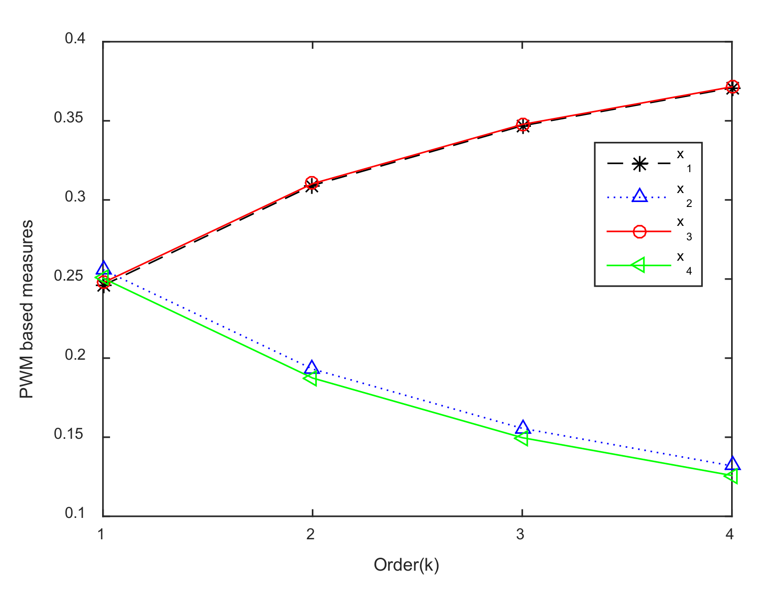
where X_i (i = 1, 2, 3, 4) all obey the exponential distribution, i.e., $X_i~Exp\left(\lambda =1\right)$. From the results shown in

Table 3. Analytical Sobol’ indices and delta indices of Example 2.

Measures	Si/STi	${\mathit{\delta }}_{\mathit{i}}$
X1	0.2500 (1)	0.1930 (1)
X2	0.2500 (1)	0.1930 (1)
X3	0.2500 (1)	0.1930 (1)
X4	0.2500 (1)	0.1930 (1)

Note: The numbers in the parentheses mean the corresponding variable’s rank of importance.

, variables have the same influence on the output according to not only the Sobol’ method but also the moment-independent method. However, measures based on PWMs are somewhat different, as presented in

Table 4. Measures based on PWMs calculated by the DLSS QMC for Example 2.

Measures	${\mathit{\eta }}_{\mathit{i}}^{\mathit{k}}$
k	1	2	3	4
X1	0.2459 (4)	0.3092 (2)	0.3469 (2)	0.3708 (2)
X2	0.2559 (1)	0.1931 (3)	0.1556 (3)	0.1319 (3)
X3	0.2476 (3)	0.3103 (1)	0.3477 (1)	0.3715 (1)
X4	0.2505 (2)	0.1874 (4)	0.1497 (4)	0.1258 (4)
Sample size	3000

and Figure 2. The variables that have absolutely the same coefficient have the same importance when ignoring the calculation and sampling error, meaning the measures can reflect the influence of positive and negative coefficients with the increase in order k.

When comparing Case 1 of Example 1 with Example 2, the former does not show much difference, although the coefficients are the same, because the PDF of the normal distribution is symmetric, while the PDF of the exponential distribution is asymmetric.

6.3. Numerical Example 3: Ishigami Function

Consider the Ishigami function [31], which is a highly nonlinear function with three inputs:

$$Y=g\left(\mathit{X}\right)=\sin \left(X_1\right)+7{\sin }^2\left(X_2\right)+0.1x_3^4\sin \left(X_1\right),$$

(21)

where X_i (i = 1, 2, 3) are uniformly distributed on interval $\left[-\pi ,\pi \right]$.

Table 5. Analytical Sobol’ indices and delta indices of Example 3.

Measures	Si	STi	${\mathit{\delta }}_{\mathit{i}}$
X1	0.3139 (2)	0.5576 (1)	0.2259 (2)
X2	0.4424 (1)	0.4424 (2)	0.4086(1)
X3	0 (3)	0.2437 (3)	0.1798 (3)

lists the Sobol’ indices calculated by the analytical method and delta indices. Measures based on PWMs calculated by the DLRS QMC are listed in

Table 6. Measures based on PWMs calculated by the DLSS QMC of Example 3.

Measures	${\mathit{\eta }}_{\mathit{i}}^{\mathit{k}}$
k	1	2	3	4
X1	0.2109 (2)	0.2126 (2)	0.2410 (2)	0.2771 (2)
X2	0.7758 (1)	0.7731 (1)	0.7348 (1)	0.6837 (1)
X3	0.013l (3)	0.0141 (3)	0.0242 (3)	0.0382 (3)
Sample size	3000

, and the corresponding figure follows. By analyzing the results, the importance rankings obtained by the main Sobol’ indices, moment-independent indices, and new measures are the same, whereas discrepancy exists with the Sobol’ total indices. This phenomenon can be explained by comparing Equation (1) with Equation (11). The definitions of the Sobol’ main index and the presented measure have a similar form, thus leading to a certain relationship between them.

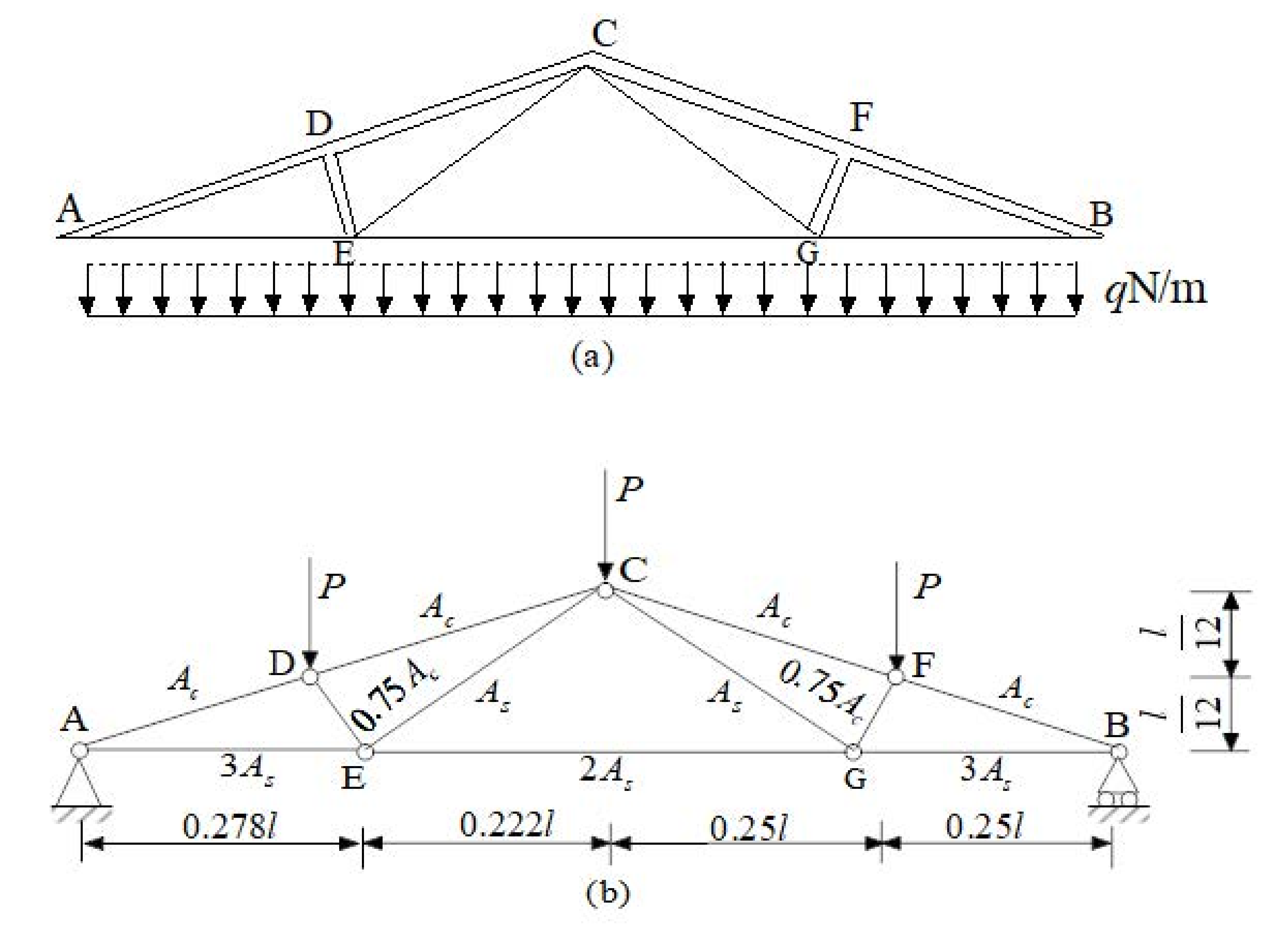
6.4. Engineering Example: A Roof Truss Structure

Consider the roof truss structure shown in Figure 3a [32]. The top boom and other compression bars are built using reinforced concrete, and the bottom boom and other tension bars are built using steel. A uniformly distributed load q is applied to the roof structure. We transform the uniform load q into a point load P = ql/4, where l is the length of the steel bars, as shown in Figure 3b. By using the first-order elastic analysis of the deformation, the vertical displacement ∆_C of the top node C can be derived as:

$${\Delta }_C=\frac{q{l}^2}{2}(\frac{3.81}{A_C{E}_C}+\frac{1.13}{A_S{E}_S}),$$

(22)

where A_C and E_C represent the sectional area and elastic modulus of concrete bars, respectively; A_S and E_S are the sectional area and elastic modulus of steel bars, respectively, which are also denoted in Figure 3b. Considering the serviceability criterion that the vertical displacement ∆_C should not exceed an admissible maximal deflection of 3 cm, the performance function can be constructed as $Y=0.03-{\Delta }_C$. Then, we assume that six random inputs q, l, A_C, E_C, A_S, and E_S are independently and normally distributed. Their distribution parameters are given in

Table 7. Distribution parameters of the roof truss structure.

Variable X	Mean	Coefficient of Variance
q (N·m−1)	20,000	0.07
l (m)	12	0.01
As (m2)	9.82 × 10−4	0.06
Ac (m2)	0.04	0.12
Es (MPa)	2 × 1011	0.06
Ec (MPa)	3 × 1010	0.06

.

Through computing four kinds of indices and rankings separately, as shown in

Table 8. List of Sobol’ indices and delta indices of Example 4.

Measures	Si	STi	${\mathit{\delta }}_{\mathit{i}}$
q	0.4581 (1)	0.4608 (1)	0.2831 (1)
l	0.0374 (5)	0.0378 (5)	0.0613 (5)
As	0.1710 (2)	0.1725 (2)	0.1427 (3)
Ac	0.1287 (4)	0.1298 (4)	0.1185 (4)
Es	0.1709 (3)	0.1724 (3)	0.1428 (2)
Ec	0.0300 (6)	0.0306 (6)	0.0541 (6)
Sample size	3 × 105

and

Table 9. Measures based on PWMs calculated by the DLSS QMC of Example 4.

Measure	${\mathit{\eta }}_{\mathit{i}}^{\mathit{k}}$
k	1	2	3	4
q	0.7657 (1)	0.7780 (1)	0.7859 (1)	0.7913 (1)
L	0.0039 (5)	0.0037 (5)	0.0035 (5)	0.0036 (5)
As	0.0891 (3)	0.0847 (3)	0.0817 (3)	0.0795 (3)
Ac	0.0491 (4)	0.0454 (4)	0.0433 (4)	0.0418 (4)
Es	0.0898 (2)	0.0858 (2)	0.0831 (2)	0.0812 (2)
Ec	0.0024 (6)	0.0025 (6)	0.0025 (6)	0.0026 (6)
Sample size	4000

, all methods have similar ranks of importance. The results show that load q is the most important input among all input variables. Thus, regarding reliability design, q should be primarily considered. Besides the load, the sectional area of concrete bars as well as the sectional area and elastic modulus of steel bars are important. The length of steel bars and the elastic modulus of concrete bars should be considered as unimportant variables, which can be treated as constant values in the optimal design. In addition, this example shows that the required sample size of measures based on PWMs is the least one among the three methods.

To summarize, the importance ranking of presented measures is usually in accordance with that of moment-independent indices ${\delta }_i$ when the PDF of the model output is symmetric or approximately symmetric. However, differences could exist if the PDF of the model output is asymmetric. In such cases, the sign of coefficients may also have an influence on PWM-based measures.

7. Conclusions

This paper introduced a novel global sensitivity measure based on PWMs. Since a PWM includes more information than a classical moment and can be accurately estimated from small samples, the new measure takes advantage of its properties. PWM-based measures can reflect the influence of input variables on output uncertainty when the output is obviously asymmetric. Subsequently, the double-loop-repeated-set QMC method and the double-loop-single-set QMC method were presented to estimate the new measure. The latter method is recommended because it needs fewer sample points. Three numerical examples were mainly used to compare the new measure with Sobol’ indices and the moment-independent delta index, thus demonstrating its advantages. Finally, an engineering example of a roof truss structure showed the possibility of realistic application. Besides, the measure can be used to analyze problems of groups of input factors.

There is still some further work that needs to be done. Detailed functions of influence factors of measures based on PWMs, i.e., PDFs and coefficients, should be found. From all the examples, the delta importance measure and presented measures often have the same ranking. So, it is possible to find a method to link them because they both identify the influence of the PDF.

References

- Saltelli, A.; Andres, M.; Campolongo, F. Global Sensitivity Analysis: The Primer; John Wiley & Sons Ltd.: Chichester, UK, 2008. [Google Scholar]
- Sobol, I.M. Sensitivity estimates for nonlinear mathematical models. Math. Model. Comput. Exp. 1993, 26, 407–414. [Google Scholar]
- Iman, R.L.; Hora, S.C. A Robust Measure of Uncertainty Importance for Use in Fault Tree System Analysis. Risk Anal. 1990, 10, 401–406. [Google Scholar] [CrossRef]
- Homma, T.; Saltelli, A. Importance measures in global sensitivity analysis of nonlinear models. Reliab. Eng. Syst. Saf. 1996, 52, 1–17. [Google Scholar] [CrossRef]
- Saltelli, A.; Tarantola, S. On the Relative Importance of Input Factors in Mathematical Models: Safety Assessment for Nuclear Waste Disposal. J. Am. Stat. Assoc. 2002, 97, 702–709. [Google Scholar] [CrossRef]
- Hang, Y.; Liu, Y.; Xu, X.; Chen, Y.; Mo, S. Sensitivity Analysis Based on Markovian Integration by Parts Formula. Math. Comput. Appl. 2017, 22, 40. [Google Scholar] [CrossRef] [Green Version]
- Cheng, K.; Lu, Z.; Ling, C.; Zhou, S. Surrogate-assisted global sensitivity analysis: An overview. Struct. Multidiscip. Optim. 2020, 61, 1187–1213. [Google Scholar] [CrossRef]
- Zhao, J.Y.; Zeng, S.K.; Guo, J.B.; Du, S. Global Reliability Sensitivity Analysis Based on Maximum Entropy and 2-Layer Polynomial Chaos Expansion. Entropy 2018, 20, 202. [Google Scholar] [CrossRef] [Green Version]
- Bhonsale, S.; López, C.A.M.; Van Impe, J. Global Sensitivity Analysis of a Spray Drying Process. Processes 2019, 7, 562. [Google Scholar] [CrossRef] [Green Version]
- Mellado, M.E.; Cisternas, L.A.; Lucay, F.A.; Gálvez, E.D. A Posteriori Analysis of Analytical Models for Heap Leaching Using Uncertainty and Global Sensitivity Analyses. Minerals 2018, 8, 44. [Google Scholar] [CrossRef] [Green Version]
- Shin, M.-J.; Choi, Y.S. Sensitivity Analysis to Investigate the Reliability of the Grid-Based Rainfall-Runoff Model. Water 2018, 10, 1839. [Google Scholar] [CrossRef] [Green Version]
- Zhou, S.; Jia, Y.; Wang, C. Global Sensitivity Analysis for the Polymeric Microcapsules in Self-Healing Cementitious Composites. Polymers 2020, 12, 2990. [Google Scholar] [CrossRef] [PubMed]
- Cox, L.A. Why risk is not variance: An expository note. Risk Anal. 2008, 28, 925–928. [Google Scholar] [CrossRef] [PubMed]
- Huber, W.A. “Why risk is not variance: An expository note” letter to editor. Risk Anal. Ysis 2010, 30, 327–328. [Google Scholar]
- Chun, M.-H.; Han, S.-J.; Tak, N.-I. An uncertainty importance measure using a distance metric for the change in a cumulative distribution function. Reliab. Eng. Syst. Saf. 2000, 70, 313–321. [Google Scholar] [CrossRef]
- Liu, H.B.; Chen, W.; Sudjianto, A. Relative entropy based method for global and regional sensitivity analysis in probabilistic design. In Proceedings of the ASME 2004 International Design Engineering Technical Conferences and Computers and Information in Engineering Conference, Salt Lake City, UT, USA, 28 September–2 October 2004; pp. 983–992. [Google Scholar]
- Borgonovo, E. A new uncertainty importance measure. Reliab. Eng. Syst. Saf. 2007, 92, 771–784. [Google Scholar] [CrossRef]
- Cui, L.; Lu, Z.; Zhao, X. Moment-independent importance measure of basic random variable and its probability density evolution solution. Sci. China Ser. E Technol. Sci. 2010, 53, 1138–1145. [Google Scholar] [CrossRef]
- Kucherenko, S.; Rodriguez-Fernandez, M.; Pantelides, C.; Shah, N. Monte Carlo evaluation of derivative based global sensitivity measures. Reliab. Eng. Syst. Saf. 2009, 94, 1135–1148. [Google Scholar] [CrossRef]
- Sobol, I.M.; Kucherenko, S. Derivative based global sensitivity measures and their link with global sensitivity indices. Math. Comput. Simul. 2009, 79, 3009–3017. [Google Scholar] [CrossRef]
- Fort, J.-C.; Klein, T.; Rachdi, N. New sensitivity analysis subordinated to a contrast. Commun. Stat. Theory Methods 2016, 45, 4349–4364. [Google Scholar] [CrossRef] [Green Version]
- Kala, Z. From Probabilistic to Quantile-Oriented Sensitivity Analysis: New Indices of Design Quantiles. Symmetry 2020, 12, 1720. [Google Scholar] [CrossRef]
- Baroni, G.; Francke, T. An effective strategy for combining variance- and distribution-based global sensitivity analysis. Environ. Model. Softw. 2020, 134, 104851. [Google Scholar] [CrossRef]
- Greenwood, J.A.; Landwehr, J.M.; Matalas, N.C.; Wallis, J.R. Probability weighted moments: Definition and relation to parameters of several distributions expressible in inverse form. Water Resour. Res. 1979, 15, 1049–1054. [Google Scholar] [CrossRef] [Green Version]
- Deng, J.; Pandey, M.D. Estimation of minimum cross-entropy quantile function using fractional probability weighted moments. Probabilistic Eng. Mech. 2009, 24, 43–50. [Google Scholar] [CrossRef]
- Pandey, M.D. Direct estimation of quantile functions using the maximum entropy principle. Struct. Saf. 2000, 22, 61–79. [Google Scholar] [CrossRef]
- Liu, Q.; Homma, T. A New Importance Measure for Sensitivity Analysis. J. Nucl. Sci. Technol. 2010, 47, 53–61. [Google Scholar] [CrossRef]
- Haktanir, T.; Bozduman, A. A study on sensitivity of the probability-weighted moments method on the choice of the plotting position formula. J. Hydrol. 1995, 168, 265–281. [Google Scholar] [CrossRef]
- Sobol, I.M. On the distribution of points in a cube and the approximate evaluation of integrals. Comput. Comput. Math. Math. Phys. 1967, 7, 86–112. [Google Scholar] [CrossRef]
- Sobol, I.M. Uniformly distributed sequences with additional uniformity properties. USSR Comput. Math. Math. Phys. 1976, 16, 236–242. [Google Scholar] [CrossRef]
- Ishigami, T.; Homma, T. An importance quantification technique in uncertainty analysis for computer models. In ISUMA’90, First International Symposium on Uncertainty Modelling and Analysis; University of Maryland: College Park, MD, USA, 1990; pp. 398–403. [Google Scholar]
- Mei, G. Research on Structural Reliability by Nonlinear Stochastic Finite Element Method; Tsinghua University: Beijing, China, 2005. (In Chinese) [Google Scholar]
Figure 1.
MaxEnt approximation combined with the PWMs of the Pareto quantile function.
Figure 2.
Measures based on PWMs under different orders for Example 2.
Figure 3.
(a) Roof truss structure and (b) distribution of loads and dimensions.