Simulation of Quasi-Static Crack Propagation by Adaptive Finite Element Method


Mechanical Engineering Department, Jazan University, Jazan 45142, Saudi Arabia
*
Author to whom correspondence should be addressed.
Metals 2021, 11(1), 98; https://doi.org/10.3390/met11010098
Submission received: 17 December 2020
/
Revised: 29 December 2020
/
Accepted: 3 January 2021
/
Published: 6 January 2021
(This article belongs to the Special Issue Computational Methods for Fatigue and Fracture)
Abstract
:The finite element method (FEM) is a widely used technique in research, including but not restricted to the growth of cracks in engineering applications. However, failure to use fine meshes poses problems in modeling the singular stress field around the crack tip in the singular element region. This work aims at using the original source code program by Visual FORTRAN language to predict the crack propagation and fatigue lifetime using the adaptive dens mesh finite element method. This developed program involves the adaptive mesh generator according to the advancing front method as well as both the pre-processing and post-processing for the crack growth simulation under linear elastic fracture mechanics theory. The stress state at a crack tip is characterized by the stress intensity factor associated with the rate of crack growth. The quarter-point singular elements are constructed around the crack tip to accurately represent the singularity of this region. Under linear elastic fracture mechanics (LEFM) with an assumption in various configurations, the Paris law model was employed to evaluate mixed-mode fatigue life for two specimens under constant amplitude loading. The framework includes a progressive analysis of the stress intensity factors (SIFs), the direction of crack growth, and the estimation of fatigue life. The results of the analysis are consistent with other experimental and numerical studies in the literature for the prediction of the fatigue crack growth trajectories as well as the calculation of stress intensity factors.
1. Introduction
The finite element method (FEM) is definitely the most common and effective analytical technique for analyzing the behavior of a wide variety of engineering and physical issues. One of the essential uses of FEM is the study of crack propagation. The propagation of the crack reduces components’ ability to resist the external load and eventually break the components. Analyzing fatigue crack growth is necessary to ensure the stability of structures subjected to cyclic loading. Cracks begin due to the presence of plastic strain caused by cyclic tension, and they grow due to the tensile stress. However, compressive loads do not lead to fatigue cracks due to the local tensile stress [1]. A variety of software has been developed for general purposes for finite elements, verified and calibrated through the years and now available on request, the most well-known being three-dimensional, such as ANSYS [2], ABAQUS [3], NASTRAN, FRANC3D, and COMSOL. In addition, there are numerous 2D simulation software for crack propagation simulation, e.g., NASGRO, AFGROW, FRANC2D, and FASTRAN. Many researchers have also developed an effective method for estimation of fatigue breakage growth in 2D linear elastic structures with multimode loading [4,5,6,7]. Determining the accurate stress intensity factor of a cracked structure in LEFM is very crucial in accessing the integrity of the crack, especially if the calculation is carried out using the finite element technique with extremely fine mesh. The propagation of the crack can be simulated at the highest accuracy by increasing the mesh density, as well as estimating the stress intensity factors accurately. In addition, very fine mesh around the crack tip is needed for precise prediction of SIFs using a nodal displacement technique such as the displacement extrapolation technique (DET). The DET requires configuration of special elements in the vicinity of the crack tip, by correctly representing the stress field singularity at the crack tip. These special elements, known as singular elements, need to be constructed in a rosette formation around every crack tip. Very small-size elements can be optimally created around the crack tip with the use of an adaptive mesh refinement scheme. Generating overall fine mesh leads to greater computational time. This procedure was reduced by using the adaptive mesh strategy, which increases the mesh only on the required areas. The adaptive mesh refinement scheme is another method to generate the optimal mesh in a very efficient way. Many studies on mesh refinement problems and related errors in computing SIFs using the FEM were conducted [8,9]. Another study [10] was been performed to clarify the effect of the in-plane and out-of-plane constraints on the ductile fracture with different crack sizes, specimen thicknesses, and span lengths. They concluded that the lower in-plane and out-of-plane constraint levels introduce higher fracture properties. It is more challenging to combine the extreme fine mesh generation with the adaptive scheme and solve the stiffness equation matrix. The benefits sought here are both faster execution time and the ability to process larger problems. In order to simulate 2D cracks under mixed mode loading, the current developed software code is formulated to allow the researcher to estimate the fatigue life and crack trajectory using the automated adaptive mesh finite element [11,12,13,14,15]. This software was created in 2004 and continues to include several features for the simulation of two-dimensional fatigue crack growth under LEFM assumptions [12,16,17,18,19,20,21]. The use of commercial software for engineers is not appropriate in at least two aspects: First, the basic algorithm that lies behind it is not fully understood, and second, the execution is completely apprehended throughout the programming ability. Commercial software can be used to model crack propagation as well, but such software is very expensive and can hardly get the source code to develop it.
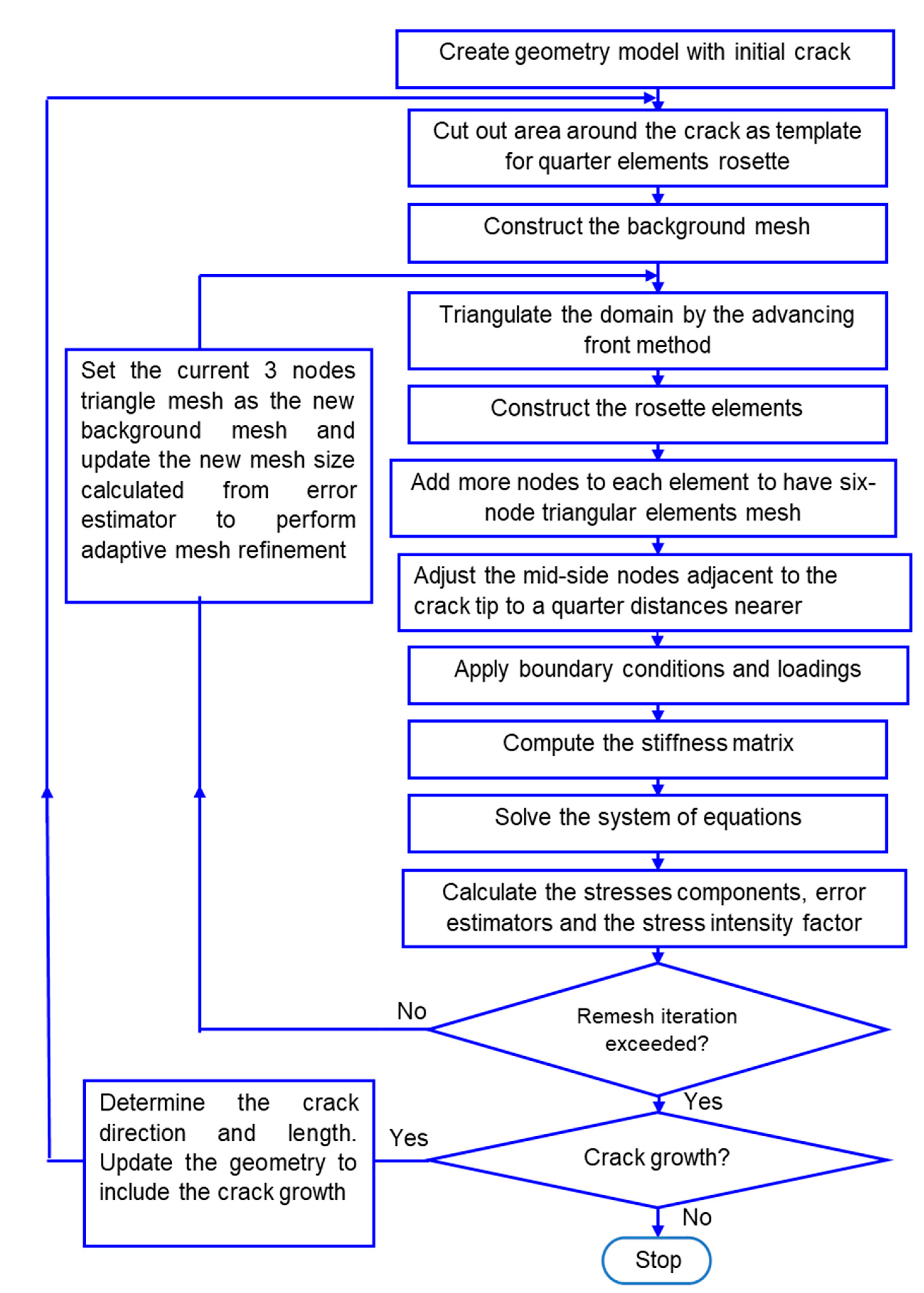
2. Developed Program Framework
The code that was developed is a simulation software to assess the 2D crack propagation process under LEFM conditions. This software predicts the growth of quasi-static crack growth in 2D components using the finite element method, taking into account the mechanical parameters of the fracture. Four essential features for the adaptive mesh finite element (FE) analysis are used for the crack direction simulation, namely, the mesh optimization algorithm, the crack criteria, the criterion of direction, and the methodology of crack propagation. The mesh refining can be controlled by the characteristic scale of each element predicted, based on the current error estimator. An incremental principle with the von Mises yield criterion is applied to this initial model. The solution errors are computed after each load stage is over. The incremental analysis is interrupted when the error exceeds a specified cumulative error at some stage and a new FE plan is generated. The program automatically configures the mesh with a new mesh refinement. After it is generated, the solution variables (displacement, stresses, strains, etc.) are transferred from the old mesh to the new mesh. The analysis is then resumed and progresses until the errors are again higher than the pre-decided amount.
In order to examine the start of the crack growth, the crack growth criterion is employed. The LEFM typically utilizes SIFs as a fracture criterion. Various techniques of estimating the path of a crack are used, such as the maximum circumferential stress theory, theory of maximum energy release, and theory of minimum energy density. At any stage of crack propagation, a FE model is defined. This model is given in the first step as an input for the modeling. The algorithm output is then generated via the models in the subsequent steps. At each stage, as the crack grows, the geometry elements are deleted and reconstructed using an adaptive technique and updated for the next propagation process. Figure 1 demonstrates the simulation procedure used to model quasi-static crack growth. The main steps of this procedure are explained in detail by [11,14].
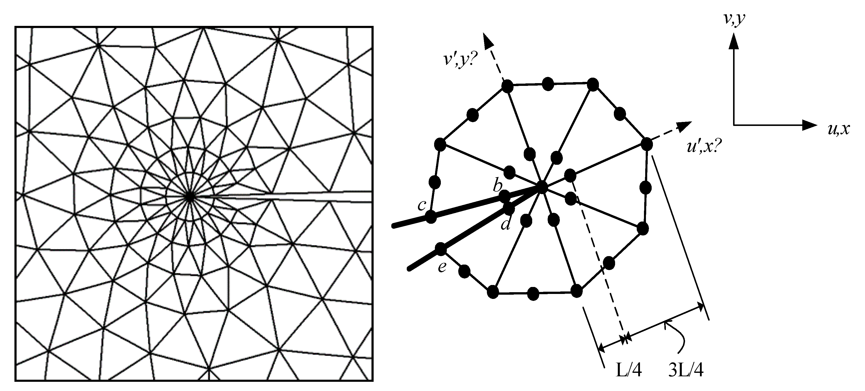
2.1. Displacement Extrapolation Technique (DET)
The DET is based on the nodal displacement around the crack tip. The construction of quarter-point elements around the crack tip is generally needed for this procedure. Generally, the existence of the quarter-point element is essential in order to correctly represent the linear elastic singularity () for stresses and strains at the crack tip. The polynomial isoparametrically representative of the singularity is typically obtained by moving the mid-side nodes adjacent to the crack tip to a quarter-length edge closer to the crack tip. Crack tip elements based on this method were separately suggested by [22,23]. In this study, the natural triangle–quarter-point element was selected as the type of crack-tip element and its configuration follows the schematic formation of the rosette around the crack-tip, as seen in Figure 2.
For the calculation of stress intensity factors, the displacement extrapolation method [24] was used as follows:
where E is the modulus of elasticity, is the Poisson’s ratio, is the elastic parameter defined by
and L is the quarter-point element length. The and are the displacement components in the x’ and y’ directions, respectively. The subscriptions represent their position, as seen in Figure 2.
2.2. Adaptive Mesh Refinement
To minimize expected errors after a finite element solution has been achieved, an adaptive mesh refinement technique is used. The method of adaptive mesh refinement measures the mesh’s adequacy and refines the mesh wherever the estimated error is large. Until user-definable error tolerance is reached, the system iterates the mesh refinement and solution. Because the precision of the solution depends on these tolerance limits, it is important for the use of adaptive mesh generators to provide a good understanding of the FEM in an effective manner. The method is referred to as adaptive since at all times the process relies on previous results. The adaptive remeshing method was carried out on the basis of the posteriori stress error standard scheme to achieve the optimum mesh from [16]. The software adopted a frontal solver that is an effective direct solver used to solve a linear equation system. In h-type adaptive mesh refinement, the major point is to obtain the ratio of element normal stress error to the average normal stress error for the entire domain, which is also known as the relative stress norm error, and a new size can be predicted from this ratio for the refinement method. The mesh size is defined in the procedure of each element as:
where is the area of the triangle element. The norm stress error for each element is defined by
whereas the average norm stress error for the whole domain is
where m indicates the total number of elements in the whole domain and is the smoothed stress vector. In the finite element treatment the integration with the isoparametric triangular element is converted by the summation of quadratures following the Radau rules [25] as follows:
where is a weighting factor and is is the Jacobian matrix.
Similarly,
where is the element thickness for a plane stress condition and for a plane strain condition. Therefore, the relative stress norm error for each item is considerably less than some identified value [26]. Thus,
And the relative stress error level of the new element is defined as permissible error as
This implies that any element with must be optimized and the new mesh size must be predicted. The asymptotic convergence rate criteria are used, which assumed
where p is the approximation of the polynomial order. In the analysis, p = 2 is used for the approximation of finite elements as a quadratic polynomial. The predicted sizes of the new element are stated as follows:
where he is the old element size and p is the order of the interpolation shape function.
Convergence of the mesh is dependent of the size of the new element, which defines how many elements in a model are required to ensure that the results of an analysis are not affected by changing the mesh size. System response (stress, deformation) converge with decreasing element size to a repeatable solution. Further refinement of the mesh does not affect results because the model and its results are now independent of the mesh.
The present mesh is known as the new background mesh and the advancing front method is replicated according to the amount of mesh refinements set by the user.
The mesh optimization is used in the final stage of the mesh generation in order to enhance the shape of the elements. The topological structure of the mesh is fixed in the process of mesh smoothing, i.e., the element’s nodal connections are not changed, but the inner nodes are repositioned to create triangles with much improved shapes. The most effective computational smoothing algorithm is the well-known Laplacian smoothing [27], which repositions the inner node created by its neighboring nodes at the center of the polygon. The new position of an internal node i is computed as
where Nn is the number of nodes linked to node i. The mesh smoothing process consists of several iterations.
2.3. Crack Growth Analysis
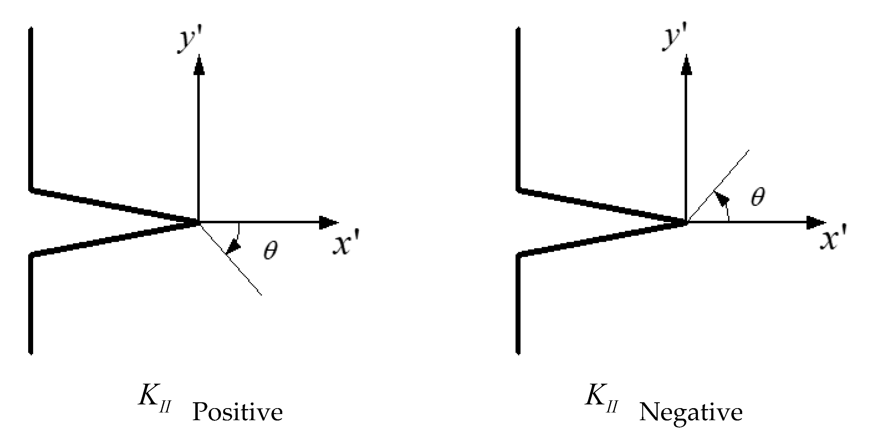
The direction of the crack path under linear elastic conditions must be computed to facilitate crack propagation simulation. The maximum circumferential stress theory states that for isotropic materials under mixed loading mode the crack grows in a direction normal to a maximum tangential tensile stress. The tangential stress is estimated in polar coordinates as
The direction normal to the tangential maximum stress can be obtained by resolving for . The nontrivial solution is determined by
which can be solved as
The sign of must be opposite the sign of to ensure the optimal opening stress associated with the crack direction [28]. Figure 3 illustrated the two possibilities of the crack growth direction.
In the case of fatigue crack growth, the resulting stress intensity range at each crack tip must exceed the stress intensity threshold, specified as
where f is a geometrical and loading function and is the stress range limit. According to Equation (17), the crack is not propagated if . This equation was practically modified by using another parameter known as the equivalent stress intensity factor range, . Therefore, if , this indicates commencement of fatigue crack growth. This parameter is set to
In the modified equation of the Paris law, Tanaka [20] derived an innovative law known as the power law for determining crack growth in response to fatigue with the equivalent stress intensity factor () as
where a is the length of the crack, N is the number of cycles, C is the Paris constant (mm/cycle), and m is the Paris exponent.
The total number of fatigue lifecycles can be calculated using Equation (19) for an increase in crack length as
3. Numerical Results and Discussion
3.1. Two Internal Non-Colinear Cracks
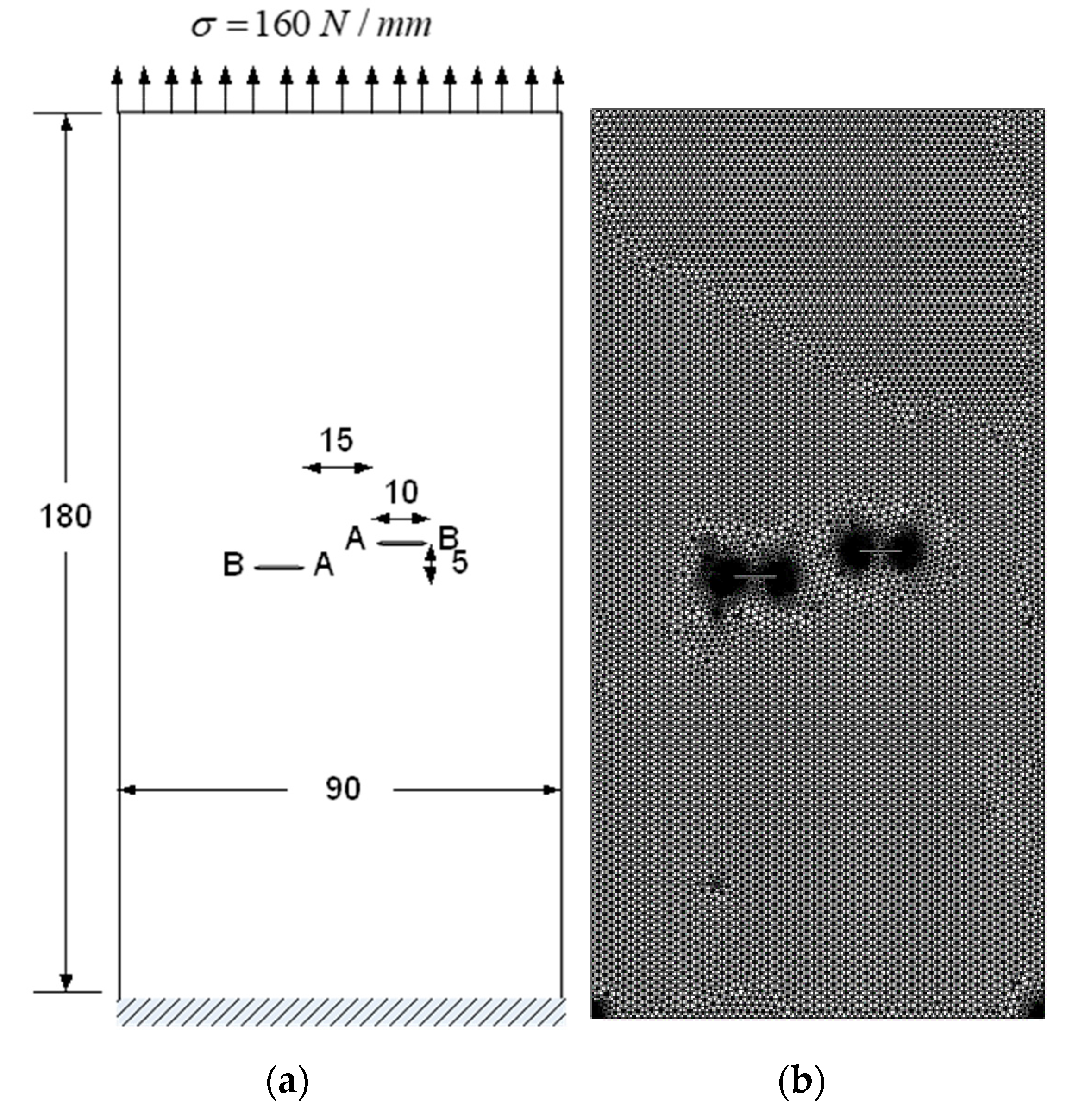
For this geometry, there were two internal, parallel, non-colinear, and non-angled cracks in a rectangular specimen with dimensions (90 mm/180 mm). The initial crack length was a = 10 mm for both cracks. As seen in Figure 4a, this geometry was subjected to acyclic tension () at the upper end and restricted at the bottom side. The distance between the two tips was 15 mm in the horizontal direction and 5 mm in the vertical direction. The adaptive dense mesh is shown in Figure 4b. The selected material was aluminum, which has the material properties shown in Table 1.
This specimen contained four crack tips, which made it interesting to observe the interaction between cracks and to further explore the performance of the developed software in the simulation of multiple cracks.
The predicted crack growth is shown in Figure 5a, which closely resembled the experimental result of Tu and Cai (1993), as illustrated in Figure 5c. These predicted crack growth trajectories were also in agreement with the numerical results obtained by [29] using the linear smoothed extended finite element method, which was compared to the numerical results reported by [5] using a meshless method with enriched weight functions, as shown in Figure 5b.
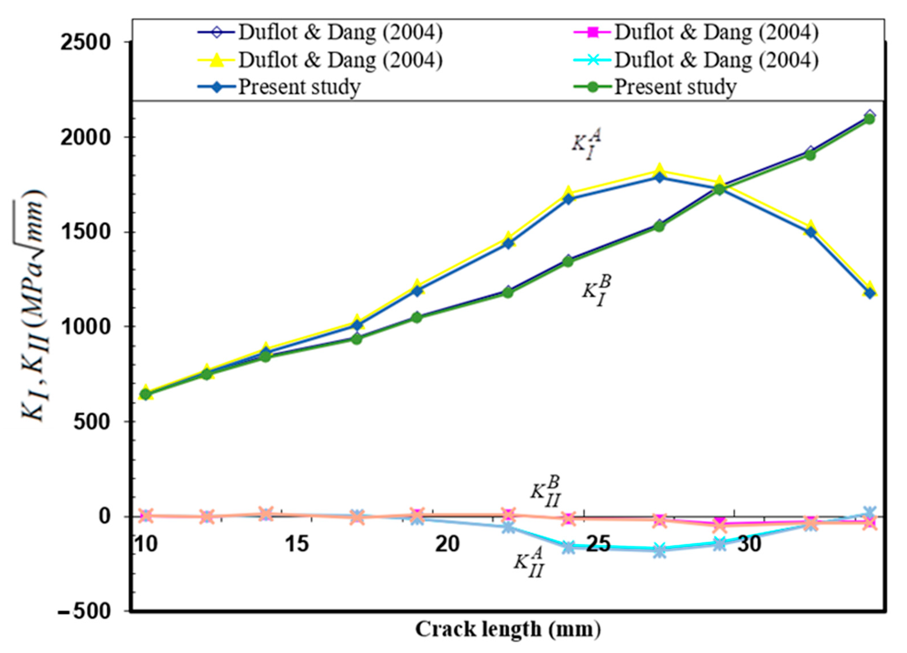
Figure 6 compares stress intensity factors in tips A and B along the crack length with the result from the meshless finite element [5]. Actually, the crack length values were the cumulative crack increment in tips A and B, starting at 10 mm in each stage, which was the original crack length. Only the upper right slip result was selected in the graph. The figure shows good agreement for the comparison results. The deviation of at a crack length of 27 mm above was attributable to the contact with the opposite crack trajectories.
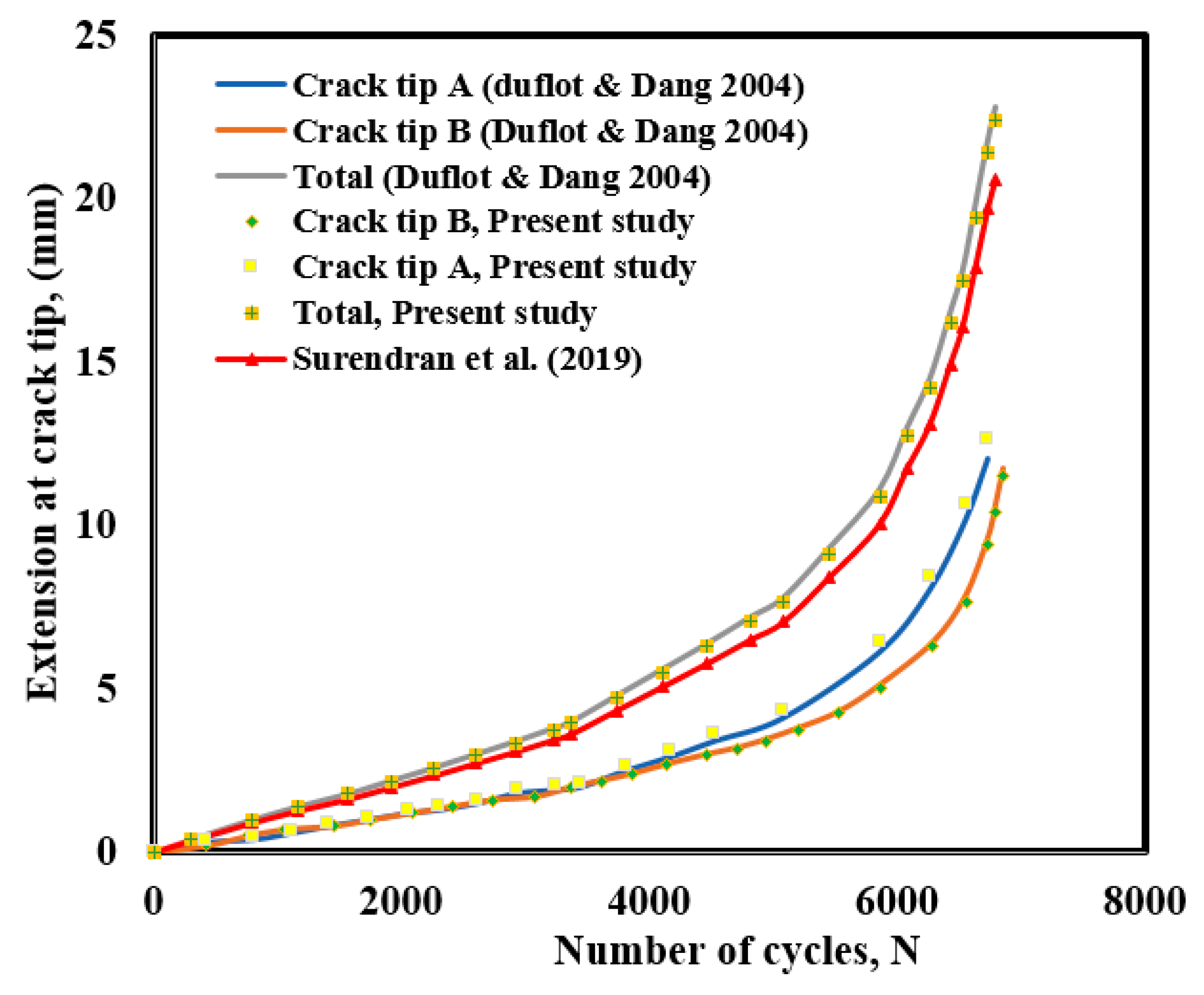
Both cracks demonstrated in the beginning a pure mode I of approximately the same SIF values. After that, the mode II of the SIF increased at tip A above that of tip B while the second mode of SIFs became negative at A, thus making the crack path curve towards the other break. Eventually the second mode of the SIFs at A tended to decrease as crack tip A moved closer when the first mode at B increased continually. Finally, the equivalent mode I of the SIF at B exceeded the fracture toughness and unstable fracture occurred at crack tip B. The fatigue life of the structure was evaluated as 6840 cycles, which was in good agreement with the results obtained by [5] using a meshless method, as shown in Figure 7, as well as with the numerical results obtained by [29].
3.2. PMMA Beam Specimen
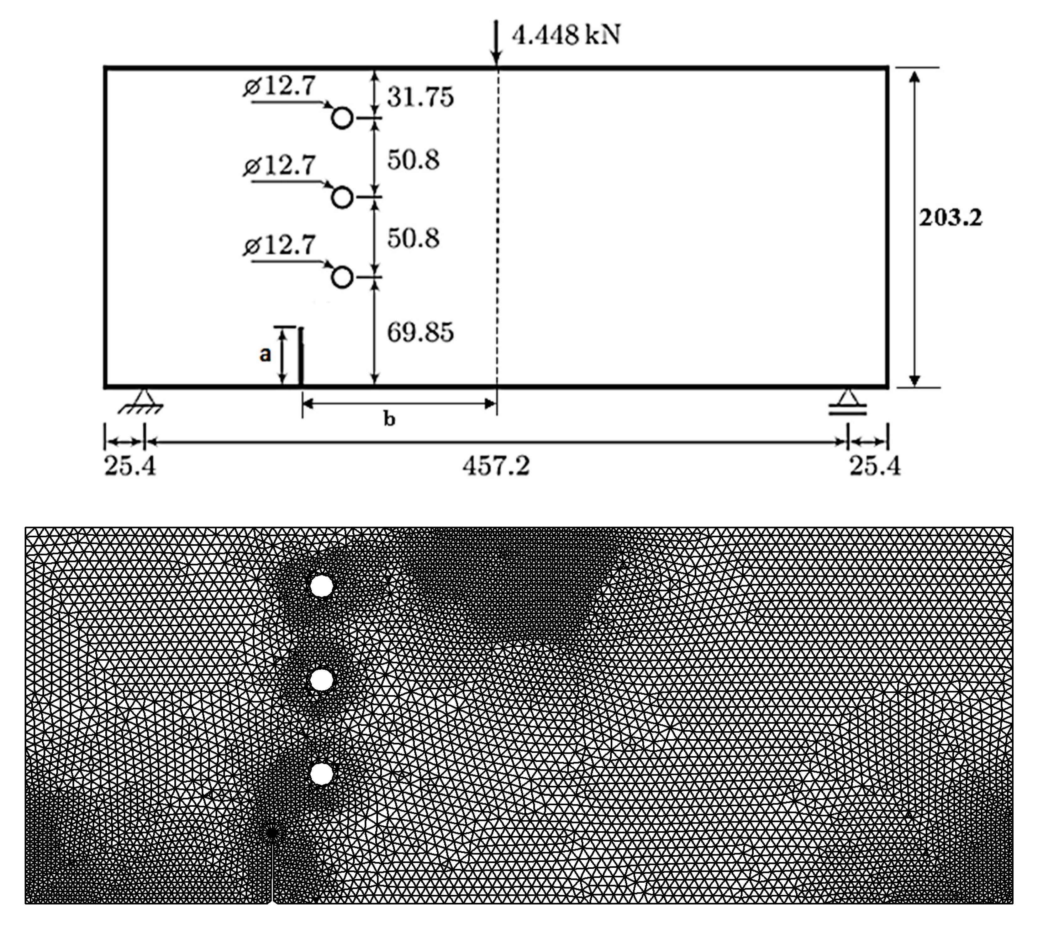
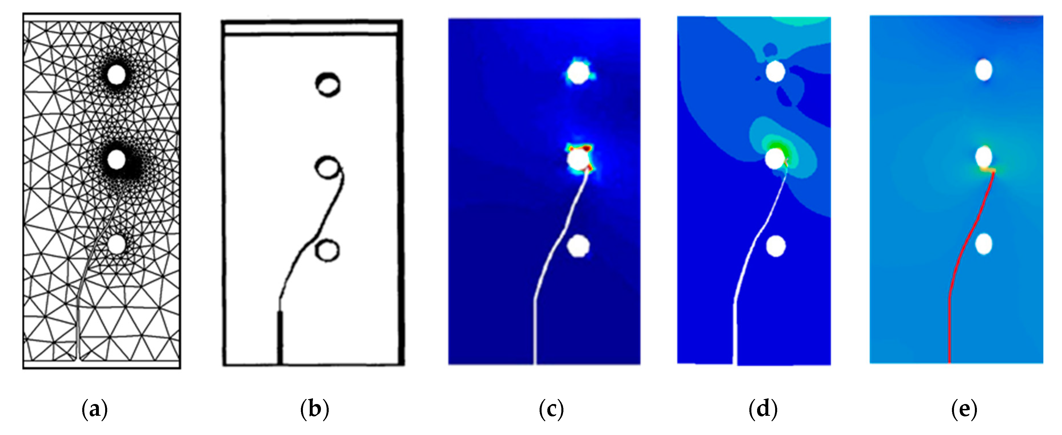
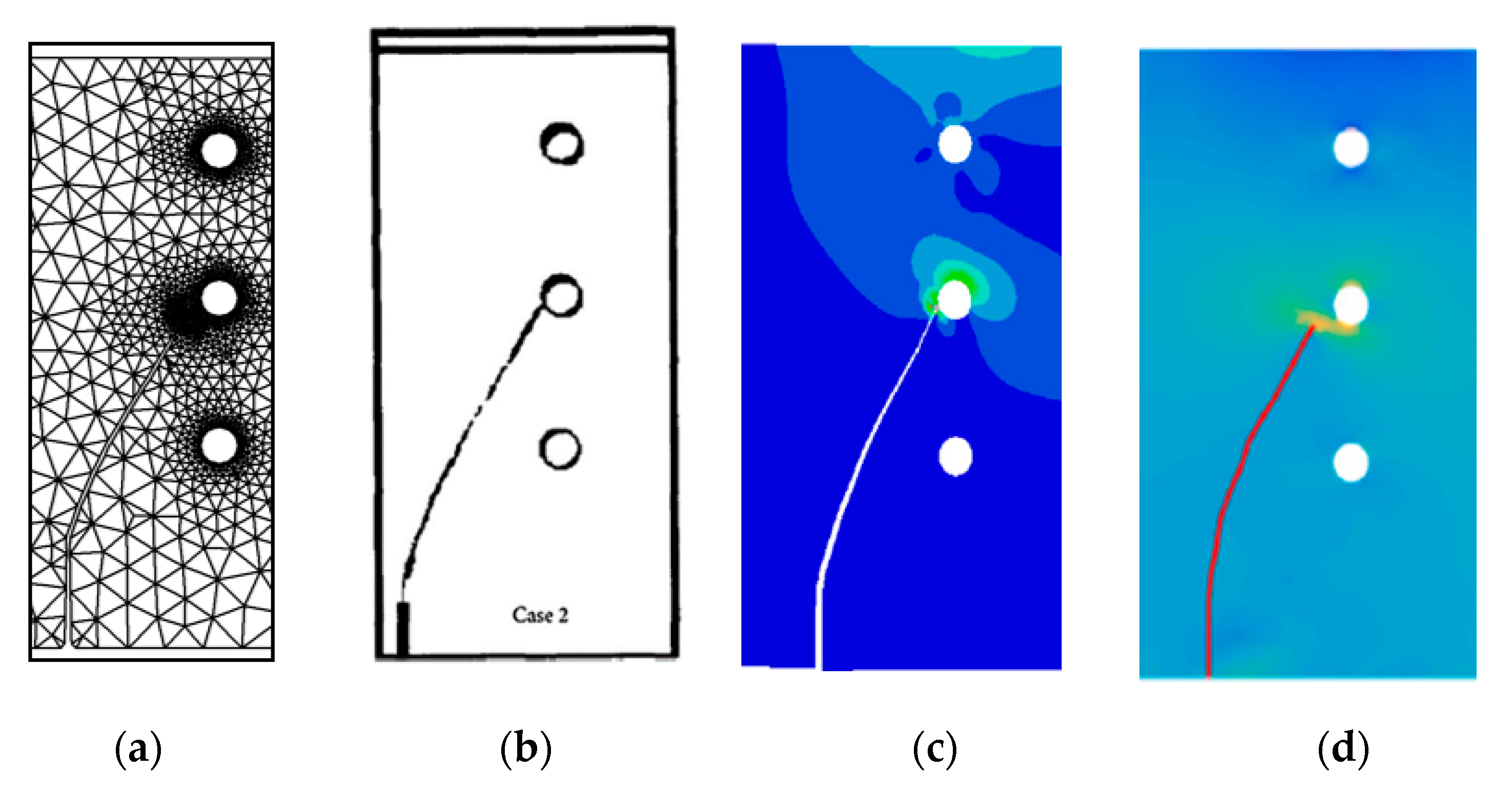
The PMMA beam geometry offers a benchmark evaluation based on the numerical and experimental work of [31]. The beams were made of polymethyl methacrylate (PMMA), which is a standard material option for crack path investigations as it is relatively homogeneous and exhibits brittle fracture behavior at room temperature. The specimen was under a cyclic point load and acted on the top mid-span position with a value of 4.448 kN. The properties of the materials were taken as modulus of elasticity, E = 205 GPa, yield stress MPa, threshold stress intensity factor , Paris law coefficient, C = 1.2 × 10⁻¹¹, Paris law exponent m = 3, and Poisson’s ratio ν = 0.3. The thickness of the specimen was 12.7 mm and there were two different configurations depending on the initial crack length (a) and its position (b), as shown in Table 2. The specimen’s geometry and the initial adaptive dens mesh are shown in Figure 8.
3.2.1. Case I
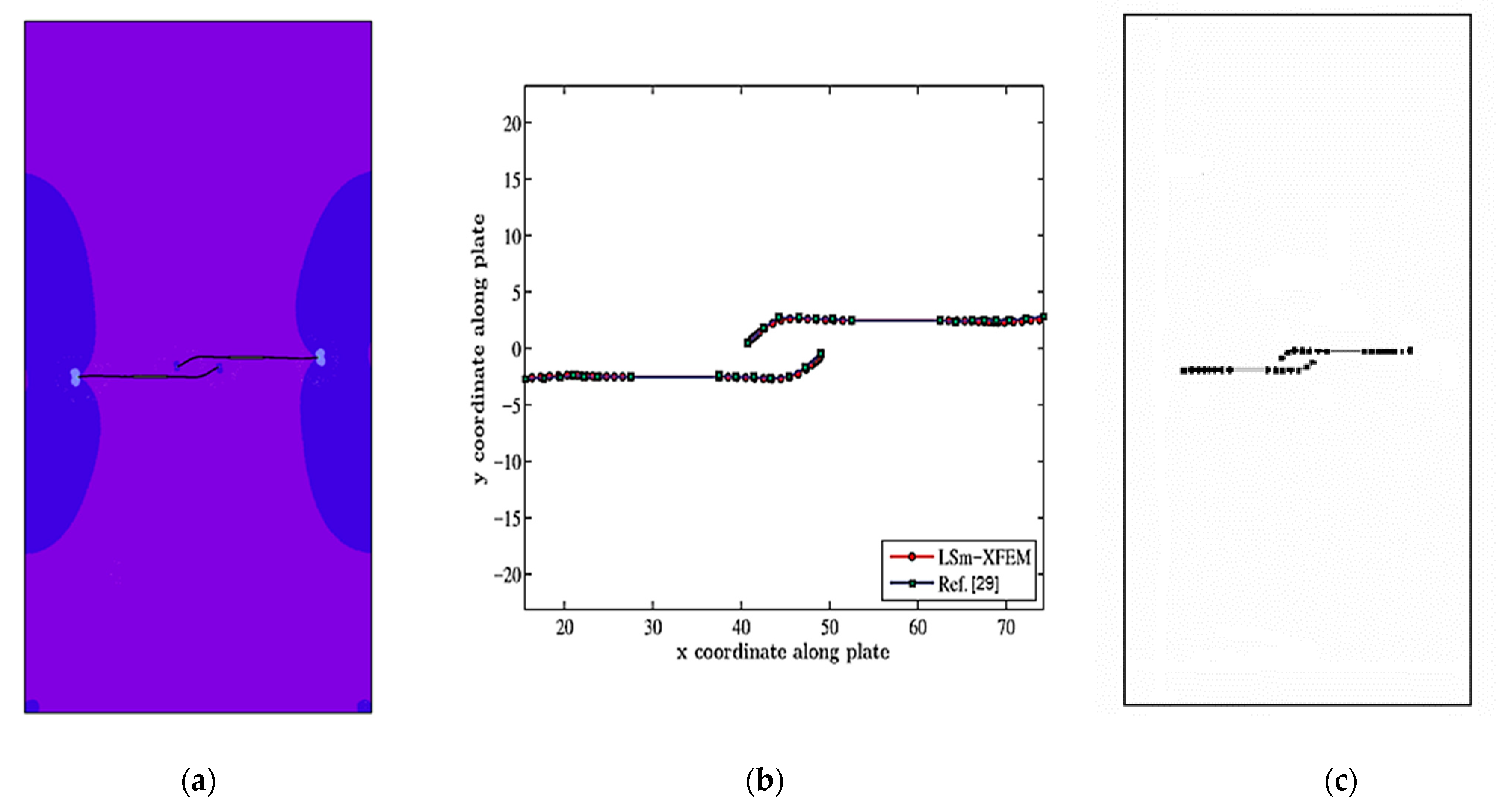
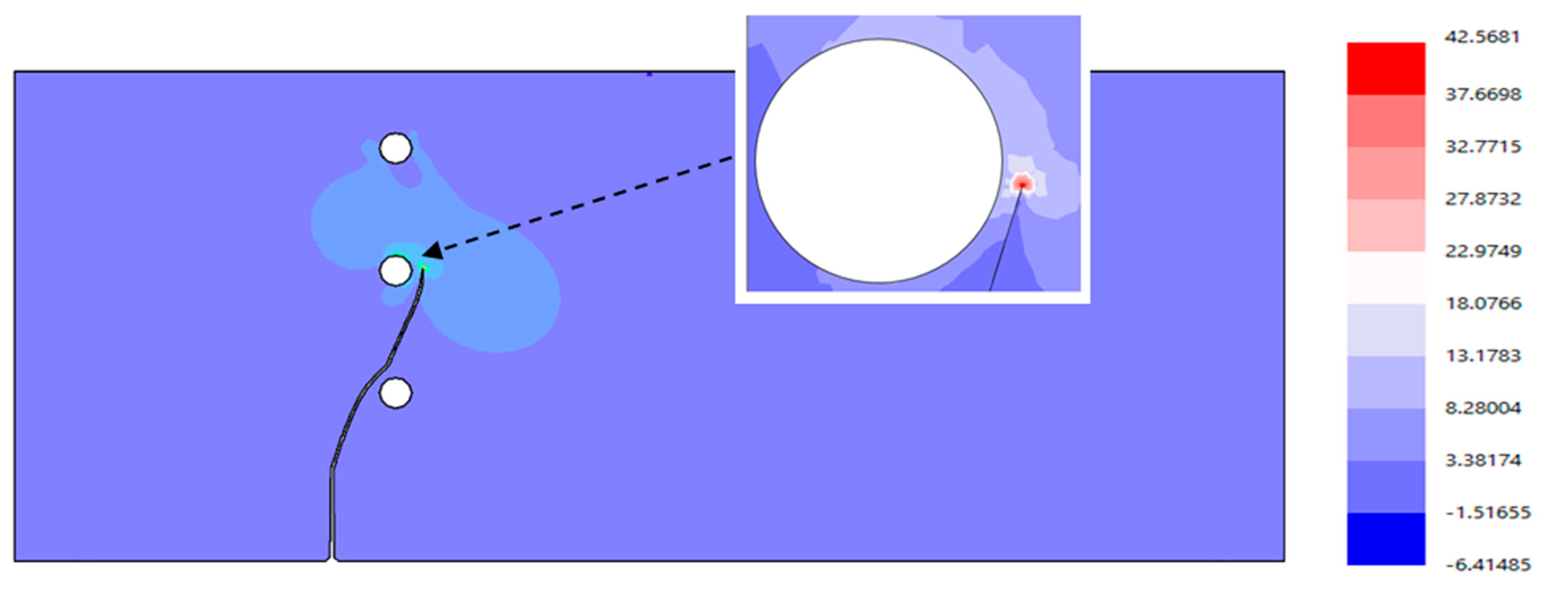
The simulated crack growth for this specimen moved between the bottom and mid-hole and reached the mid-hole on the right side. It presented a significant increase in the KII component of the shear stress intensity factor across the cracks, which forced the step-sizes of the crack to be shortened. The findings of the crack trajectory during propagation were excellently consistent with the experimental results of the crack trajectory [32], the numerical results obtained by [33] using A polygonal extended finite element method (XFEM) with numerical integration for linear elastic fracture mechanics, the XFEM results using ABAQUS software obtained by obtained by [34], and with the numerical results using the coupled extended meshfree–smoothed meshfree method presented by [35], as shown in Figure 9a–e, respectively. The maximum principal stress distribution is shown in Figure 10.
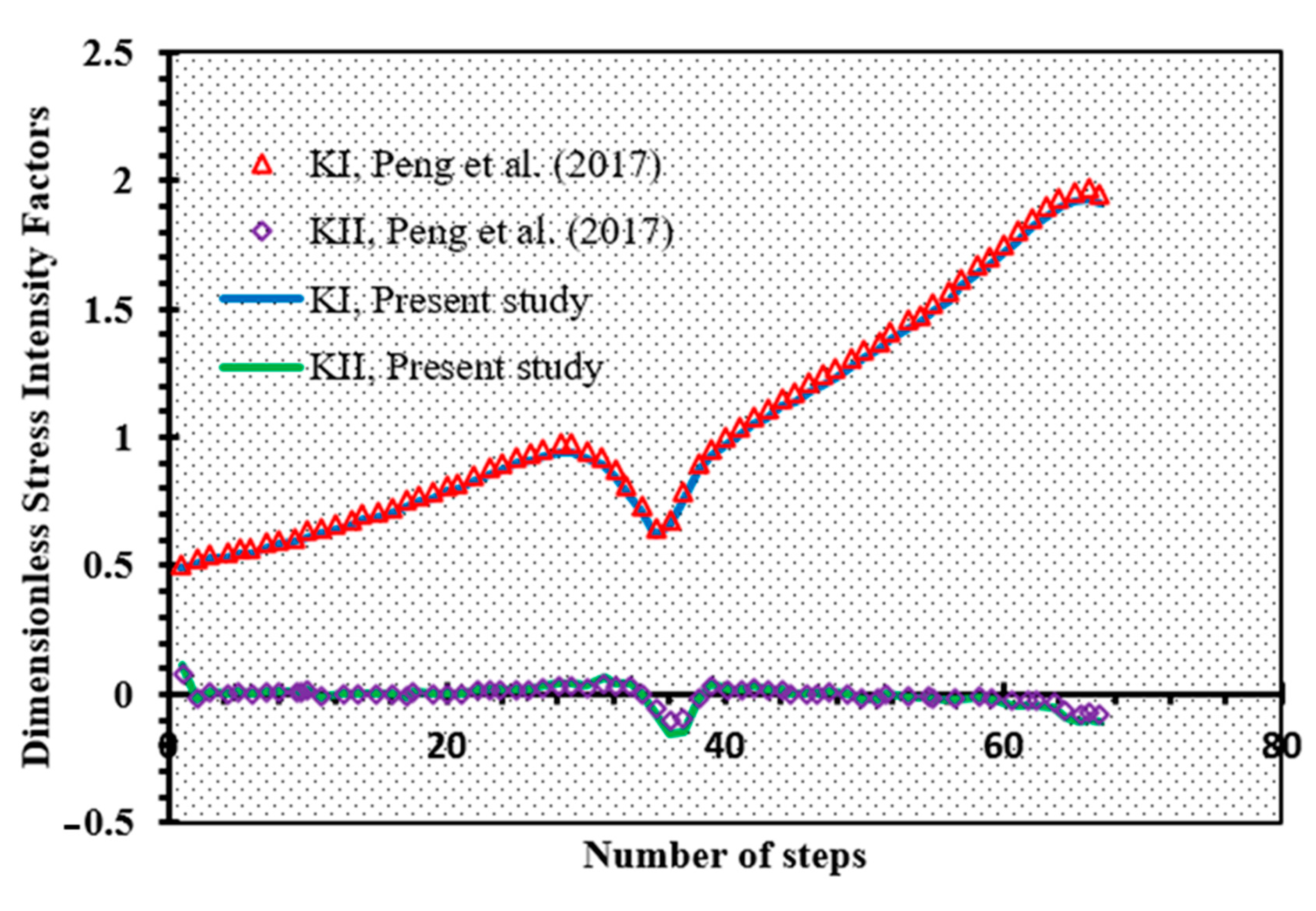
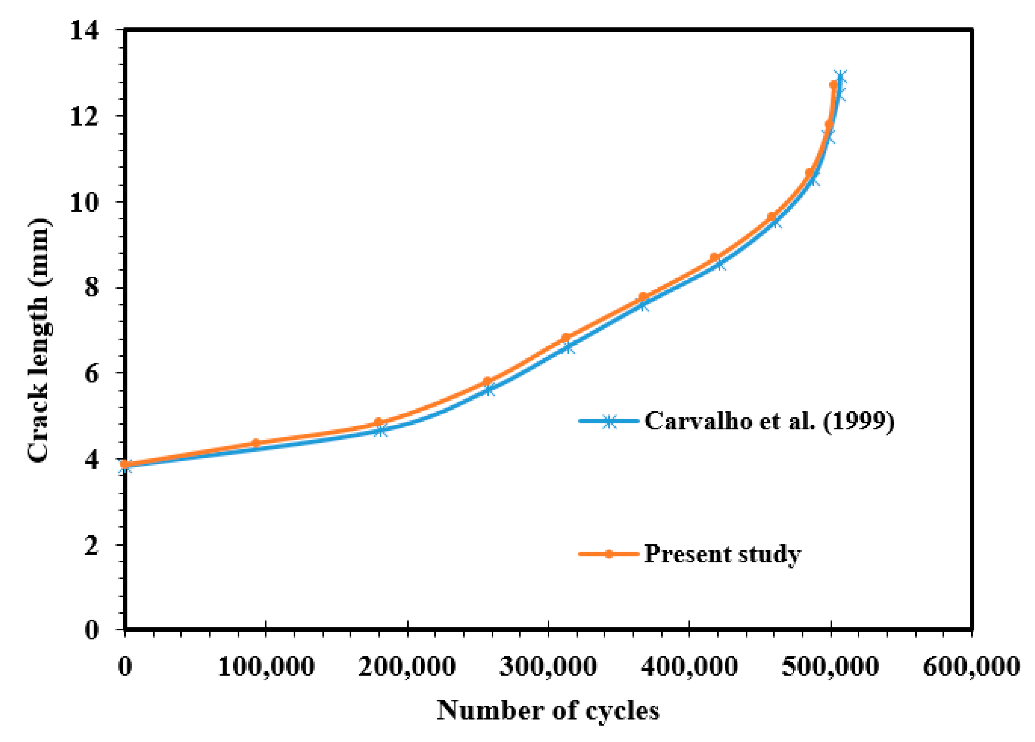
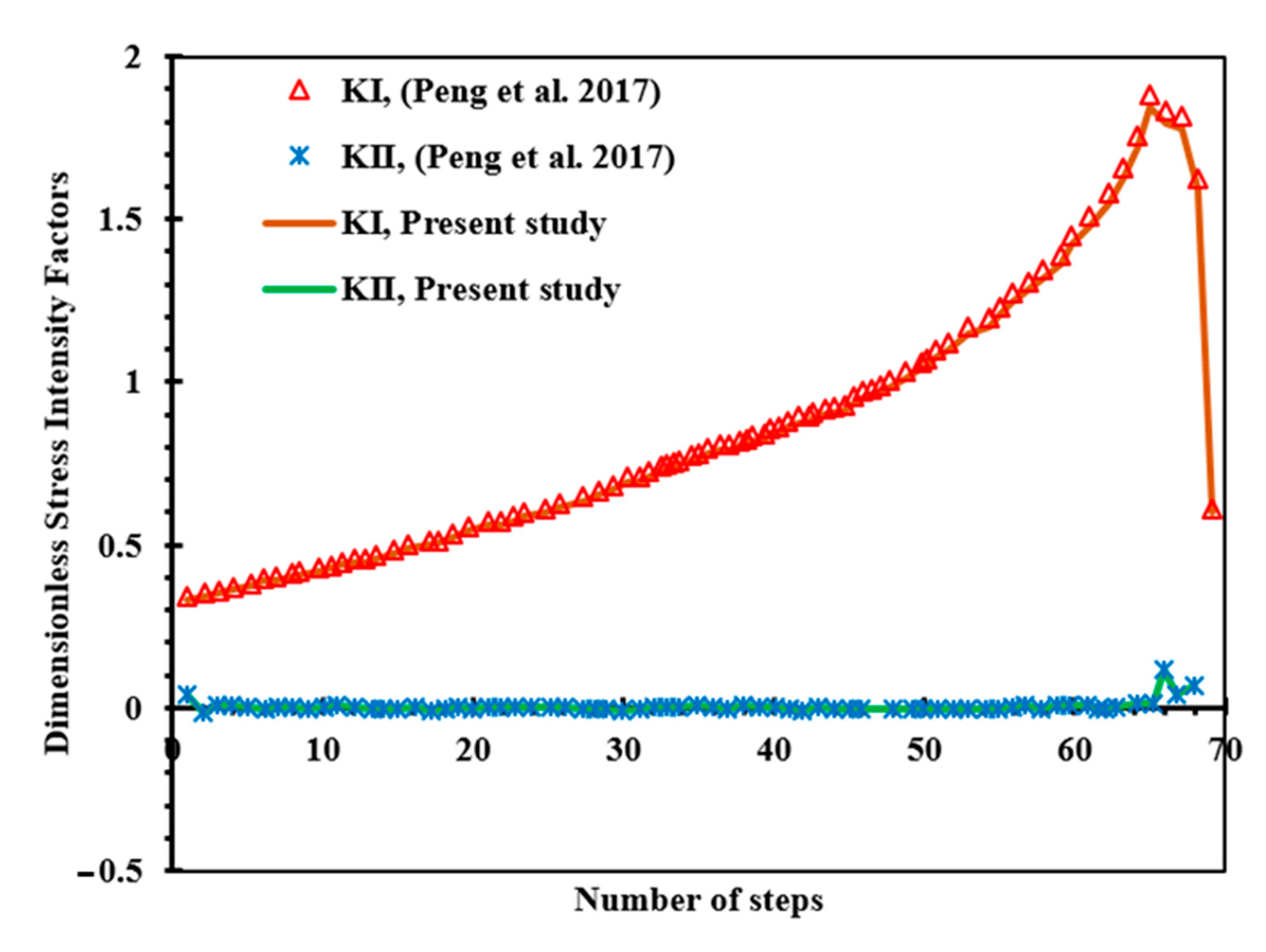
The results of this simulation were compared with those from XFEM using the smooth nodal stress technique by Peng et al. 2017, as shown in Figure 11, with good agreement. It was found that as the crack approached the hole, the SIFs appeared to change to a greater amplitude. The predicted fatigue life for this specimen was compared to the analytical results calculated by [36] using Paris and Walker models, as shown in Figure 12, with good agreement.
3.2.2. Case II
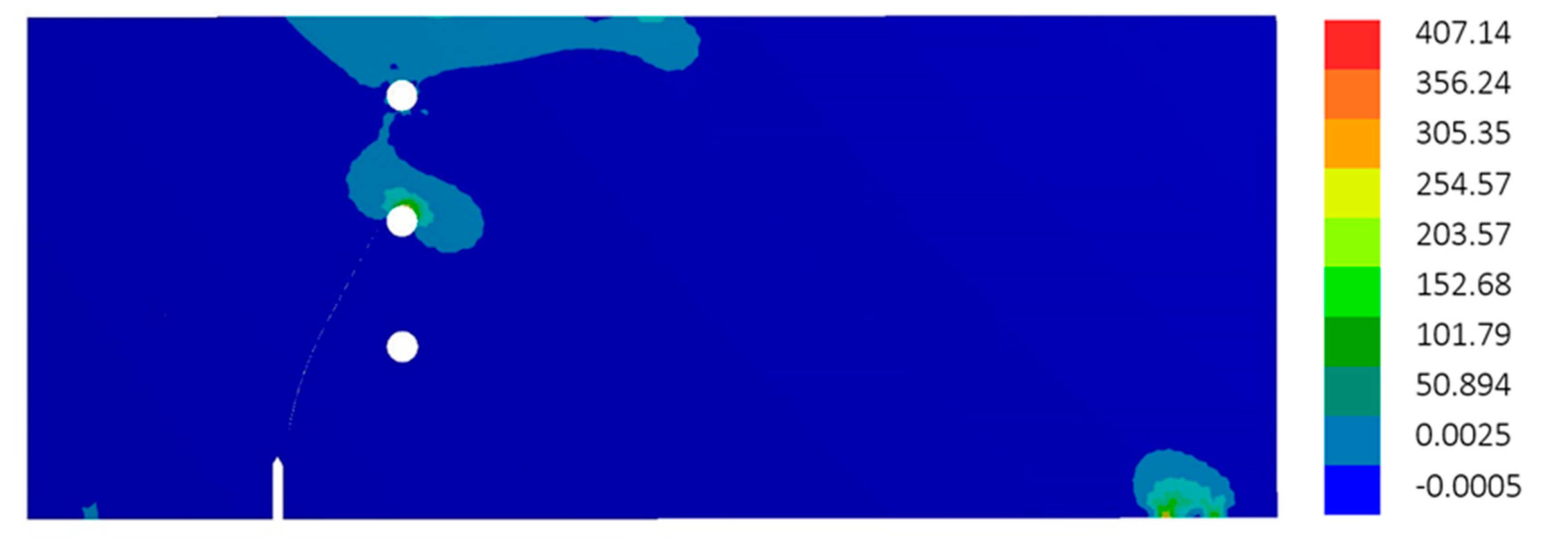
According to Table 2, the differences between this case and the previous case were the initial crack length and its position from the mid-span, which were 38.1 mm and 127 mm, respectively. The crack moved above the lower hole in this specimen and stopped at the central hole from the left. The results of the crack trajectory during propagation were excellently close to the experimental results of the crack trajectory obtained by [32], XFEM results using ABAQUS software obtained by [34], as well as the numerical results obtained by [35] using the coupled extended meshfree–smoothed meshfree method, as shown in Figure 13a–d, respectively. The distribution of the von Mises stress is shown in Figure 14.
4. Conclusions
The results of the developed program simulation were compared with experimental and numerical data for the two internal non-colinear cracks and the three-point bending beam with three holes with two different configurations. The developed program combines the adaptive mesh refinement with increasing mesh density in the required area only in order to reduce the computational time while increasing the solution accuracy. The norm stress error is taken as a posterior estimator for the h-type adaptive refinement. With this series of simulations, the capability of the developed program was demonstrated to accurately predict the crack path trajectory, stress intensity factors, and fatigue life under constant amplitude loading. In these simulation sequences, holes act as a crack stopper and attract a crack trajectory to growth. Such findings support that the algorithm can be used to identify crack-stopping holes used in damage tolerance designs.
Author Contributions
Conceptualization, A.M.A.; methodology, A.M.A.; software, A.M.A.; validation, A.M.A., and Y.A.F.; formal analysis, A.M.A.; investigation, A.M.A. and Y.A.F.; resources, A.M.A.; data curation, A.M.A. and Y.A.F.; writing—original draft preparation, A.M.A.; writing—review and editing, A.M.A. and Y.A.F.; visualization, A.M.A. and Y.A.F.; supervision, A.M.A.; project administration, A.M.A. and Y.A.F.; funding acquisition, A.M.A. and Y.A.F. Both authors have read and agreed to the published version of the manuscript.
Funding
This research received no external funding.
Institutional Review Board Statement
Not applicable.
Informed Consent Statement
Informed consent was obtained from all subjects involved in the study.
Data Availability Statement
The data presented in this study are available in the article.
Conflicts of Interest
The authors declare no conflict of interest.
References
- Liu, A.F. Mechanics and Mechanisms of Fracture: An Introduction; ASM International: Geauga County, OH, USA, 2005. [Google Scholar]
- ANSYS. Academic Research Mechanical, Release 19.2, Help System. In Coupled Field Analysis Guide; ANSYS, Inc.: Canonsburg, PA, USA, 2020. [Google Scholar]
- Manual, A.U. Abaqus User Manual; Abacus: Waltham, MA, USA, 2020. [Google Scholar]
- Lebaillif, D.; Recho, N. Brittle and ductile crack propagation using automatic finite element crack box technique. Eng. Fract. Mech. 2007, 74, 1810–1824. [Google Scholar] [CrossRef]
- Duflot, M.; Nguyen-Dang, H. Fatigue crack growth analysis by an enriched meshless method. J. Comput. Appl. Math. 2004, 168, 155–164. [Google Scholar] [CrossRef] [Green Version]
- Yan, X. Automated simulation of fatigue crack propagation for two-dimensional linear elastic fracture mechanics problems by boundary element method. Eng. Fract. Mech. 2007, 74, 2225–2246. [Google Scholar] [CrossRef]
- Zhao, T.; Zhang, J.; Jiang, Y. A study of fatigue crack growth of 7075-T651 aluminum alloy. Int. J. Fatigue 2008, 30, 1169–1180. [Google Scholar] [CrossRef]
- Miranda, A.C.D.O.; Meggiolaro, M.A.; Martha, L.F.; Castro, J. Stress intensity factor predictions: Comparison and round-off error. Comput. Mater. Sci. 2012, 53, 354–358. [Google Scholar] [CrossRef]
- Ingraffea, A.R.; de Borst, R. Computational Fracture mechanics. In Encyclopedia of Computational Mechanics, 2nd ed.; John Wiley & Sons, Ltd.: West Sussex, UK, 2017; pp. 1–26. [Google Scholar]
- Liu, Z.; Wang, X.; Miller, R.E.; Hu, J.; Chen, X. Ductile fracture properties of 16MND5 bainitic forging steel under different in-plane and out-of-plane constraint conditions: Experiments and predictions. Eng. Fract. Mech. 2021, 241, 107359. [Google Scholar] [CrossRef]
- Alshoaibi, A.M. Finite element procedures for the numerical simulation of fatigue crack propagation under mixed mode loading. Struct. Eng. Mech. 2010, 35, 283–299. [Google Scholar] [CrossRef]
- Alshoaibi, A.M. An Adaptive Finite Element Framework for Fatigue Crack Propagation under Constant Amplitude Loading. Int. J. Appl. Sci. Eng. 2015, 13, 261–270. [Google Scholar]
- Alshoaibi, A. Finite element-based model for crack propagation in linear elastic materials. Eng. Solid Mech. 2020, 8, 131–142. [Google Scholar] [CrossRef]
- Alshoaibi, A.M.; Hadi, M.; Ariffin, A. Two-dimensional numerical estimation of stress intensity factors and crack propagation in linear elastic Analysis. J. Struct. Durab. Health Monit. 2007, 3, 15–27. [Google Scholar]
- Fageehi, Y.A.; Alshoaibi, A.M. Nonplanar Crack Growth Simulation of Multiple Cracks Using Finite Element Method. Adv. Mater. Sci. Eng. 2020, 2020, 1–12. [Google Scholar] [CrossRef] [Green Version]
- Alshoaibi, A.M.; Ariffin, A. Finite element modeling of fatigue crack propagation using a self adaptive mesh strategy. Int. Rev. Aerosp. Eng. 2015, 8, 209–215. [Google Scholar] [CrossRef]
- Alshoaibi, A.M.; Ariffin, A. Fatigue life and crack path prediction in 2D structural components using an adaptive finite element strategy. Int. J. Mech. Mater. Eng. 2008, 3, 97–104. [Google Scholar]
- Alshoaibi, A.M.; Ariffin, A.K. Finite element simulation of stress intensity factors in elastic-plastic crack growth. J. Zhejiang Univ. Sci. A 2006, 7, 1336–1342. [Google Scholar] [CrossRef]
- Alshoaibi, A.M. A two dimensional Simulation of crack propagation using Adaptive Finite Element Analysis. J. Comput. Appl. Mech. 2018, 49, 335–341. [Google Scholar]
- Alshoaibi, A.M.; Fageehi, Y.A. Fageehi, 2D finite element simulation of mixed mode fatigue crack propagation for CTS specimen. J. Mater. Res. Technol. 2020, 9, 7850–7861. [Google Scholar] [CrossRef]
- Bashiri, A.H.; Alshoaibi, A.M. Adaptive Finite Element Prediction of Fatigue Life and Crack Path in 2D Structural Components. Metals 2020, 10, 1316. [Google Scholar] [CrossRef]
- Barsoum, R.S. Application of quadratic isoparametric finite elements in linear fracture mechanics. Int. J. Fract. 1974, 10, 603–605. [Google Scholar] [CrossRef]
- Henshell, R.D.; Shaw, K.G. Crack tip finite elements are unnecessary. Int. J. Numer. Methods Eng. 1975, 9, 495–507. [Google Scholar] [CrossRef]
- Phongthanapanich, S.; Dechaumphai, P. Adaptive Delaunay triangulation with object-oriented programming for crack propagation analysis. Finite Elements Anal. Des. 2004, 40, 1753–1771. [Google Scholar] [CrossRef]
- Erdogan, F.; Sih, G.C. On the crack extension in plates under plane loading and transverse shear. J. Basic Eng. 1963, 85, 519–525. [Google Scholar] [CrossRef]
- Zienkiewicz, O.; Taylor, R.; Zhu, J. The Finite Element Method: Its Basis and Fundamentals; Elsevier: Amsterdam, The Netherlands, 2005. [Google Scholar]
- Cavendish, J.C. Automatic triangulation of arbitrary planar domains for the finite element method. Int. J. Numer. Methods Eng. 1974, 8, 679–696. [Google Scholar] [CrossRef]
- Andersen, M.R. Fatigue Crack Initiation and Growth in Ship Structures; Department of Naval Architecture and Offshore Engineering, Technical University of Denmark: Lyngby, Denmark, 1998. [Google Scholar]
- Surendran, M.; Bordas, S.; Palani, G.; Bordas, S. Linear smoothed extended finite element method for fatigue crack growth simulations. Eng. Fract. Mech. 2019, 206, 551–564. [Google Scholar] [CrossRef]
- Tu, S.; Cai, R. A coupling of boundary elements and singular integral equation for the solution of the fatigue cracked body. Stress Anal. 1993, 3, 239–247. [Google Scholar]
- Bittencourt, T.; Wawrzynek, P.; Ingraffea, A.; Sousa, J. Quasi-automatic simulation of crack propagation for 2D LEFM problems. Eng. Fract. Mech. 1996, 55, 321–334. [Google Scholar] [CrossRef]
- Ingraffea, A.R.; Grigoriu, M. Probabilistic Fracture Mechanics: A Validation of Predictive Capability; Cornell University Ithaca Ny Depterment of Structural Engineering: Ithaca, NY, USA, 1990. [Google Scholar]
- Huynh, H.D.; Nguyen, M.N.; Cusatis, G.; Tanaka, S.; Bui, T.Q. A polygonal XFEM with new numerical integration for linear elastic fracture mechanics. Eng. Fract. Mech. 2019, 213, 241–263. [Google Scholar] [CrossRef]
- Dirik, H.; Yalçinkaya, T. Crack path and life prediction under mixed mode cyclic variable amplitude loading through XFEM. Int. J. Fatigue 2018, 114, 34–50. [Google Scholar] [CrossRef]
- Ma, W.; Liu, G.; Wang, W. A coupled extended meshfree–Smoothed meshfree method for crack growth simulation. Theor. Appl. Fract. Mech. 2020, 107, 102572. [Google Scholar] [CrossRef]
- Carvalho, C.V.; de Araújo, T.D.P.; Cavalcante, J.B.; Martha, L.F.; Bittencourt, T. Automatic Fatigue Crack Propagation Using a Self-Adaptative Strategy. In Proceedings of the PACAM VI––Sixth Pan-American Congress of Applied Mechanics, Rio de Janeiro, Brazial; 1999. Available online: file:///C:/Users/MDPI/AppData/Local/Temp/Automatic_fatigue_crack_propagation_using_a_self-a.pdf (accessed on 15 October 2020).
- Peng, X.; Kulasegaram, S.; Wu, S.; Bordas, S. An extended finite element method (XFEM) for linear elastic fracture with smooth nodal stress. Comput. Struct. 2017, 179, 48–63. [Google Scholar] [CrossRef] [Green Version]
Figure 1.
General flow chart of the quasi-static crack growth program.

Figure 2.
A quarter-point singular element around the tip of the crack.

Figure 3.
Sign of the crack growth angle.

Figure 4.
(a) Problem statement for two internal non-colinear cracks (all dimensions in mm) and (b) adaptive mesh for the specimen.
Figure 4.
(a) Problem statement for two internal non-colinear cracks (all dimensions in mm) and (b) adaptive mesh for the specimen.

Figure 5.
(a) Crack propagation simulation for the two internal non-colinear cracks specimen, (b) the numerical results of [29], with permission from Elsevier 2019, and (c) the experimental results [30].

Figure 6.
SIFs versus crack length comparison between the present study and the results of [5] for the two internal non-colinear crack specimens.
Figure 6.
SIFs versus crack length comparison between the present study and the results of [5] for the two internal non-colinear crack specimens.

Figure 7.
Comparison for the fatigue lifecycles for the two internal non-colinear cracks.

Figure 8.
Problem statement for the PMMA specimen (dimensions in mm) and initial adaptive dens mesh.
Figure 8.
Problem statement for the PMMA specimen (dimensions in mm) and initial adaptive dens mesh.

Figure 9.
Final crack growth path for case I: (a) present study, (b) experimental results [32], (c) [33] with permission of Elsevier 2019, (d) [34] with permission of Elsevier 2018, and (e) [35] with permission of Elsevier 2020.

Figure 10.
Maximum principal stress distribution of case I for the PMMA specimen.

Figure 11.
Non-dimensional stress intensity factors for case I of the PMMA specimen.

Figure 12.
Predicted crack growth path for case I of the PMMA specimen.

Figure 13.
Final crack growth path for case I: (a) present study, (b) experimental results [32], (c) [34] with permission of Elsevier 2018, and (e) [35] with permission of Elsevier 2020.

Figure 14.
Von Mises stress distribution of case II for the PMMA specimen.

Figure 15.
Comparison of the dimensionless stress intensity factors for case II for the PMMA specimen.
Figure 15.
Comparison of the dimensionless stress intensity factors for case II for the PMMA specimen.


Table 1.
Material properties of aluminum.
| Property | Value in Metric Unit |
|---|---|
| Modulus of elasticity, E | 74 GPa |
| Poisson’s ratio, υ | 0.3 |
| Fracture toughness, KIC | |
| Threshold stress intensity factor, Kth | |
| Paris law coefficient, C | 2.087136 × 10⁻¹³ |
| Paris law exponent m | 3.32 |
Table 2.
Configurations of the PMMA specimen.
| Specimen | a | b |
|---|---|---|
| Case I | 25.4 | 152.4 |
| Case II | 38.1 | 127 |
Publisher’s Note: MDPI stays neutral with regard to jurisdictional claims in published maps and institutional affiliations. |
© 2021 by the authors. Licensee MDPI, Basel, Switzerland. This article is an open access article distributed under the terms and conditions of the Creative Commons Attribution (CC BY) license (http://creativecommons.org/licenses/by/4.0/).
Share and Cite
MDPI and ACS Style
Alshoaibi, A.M.; Fageehi, Y.A. Simulation of Quasi-Static Crack Propagation by Adaptive Finite Element Method. Metals 2021, 11, 98. https://doi.org/10.3390/met11010098
AMA Style
Alshoaibi AM, Fageehi YA. Simulation of Quasi-Static Crack Propagation by Adaptive Finite Element Method. Metals. 2021; 11(1):98. https://doi.org/10.3390/met11010098
Chicago/Turabian StyleAlshoaibi, Abdulnaser M., and Yahya Ali Fageehi. 2021. "Simulation of Quasi-Static Crack Propagation by Adaptive Finite Element Method" Metals 11, no. 1: 98. https://doi.org/10.3390/met11010098
Note that from the first issue of 2016, this journal uses article numbers instead of page numbers. See further details here.