Determining Cover Management Factor with Remote Sensing and Spatial Analysis for Improving Long-Term Soil Loss Estimation in Watersheds


Abstract
:1. Introduction
2. Methods
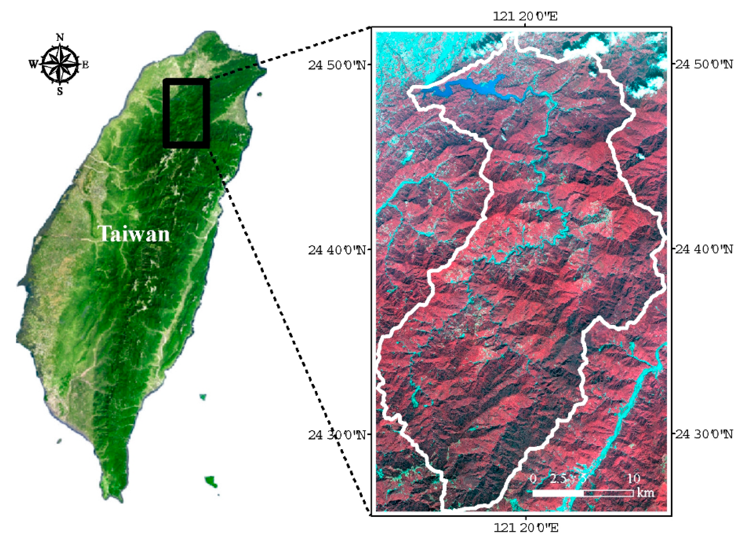
2.1. Study Area
2.2. Materials and Data Preprocessing
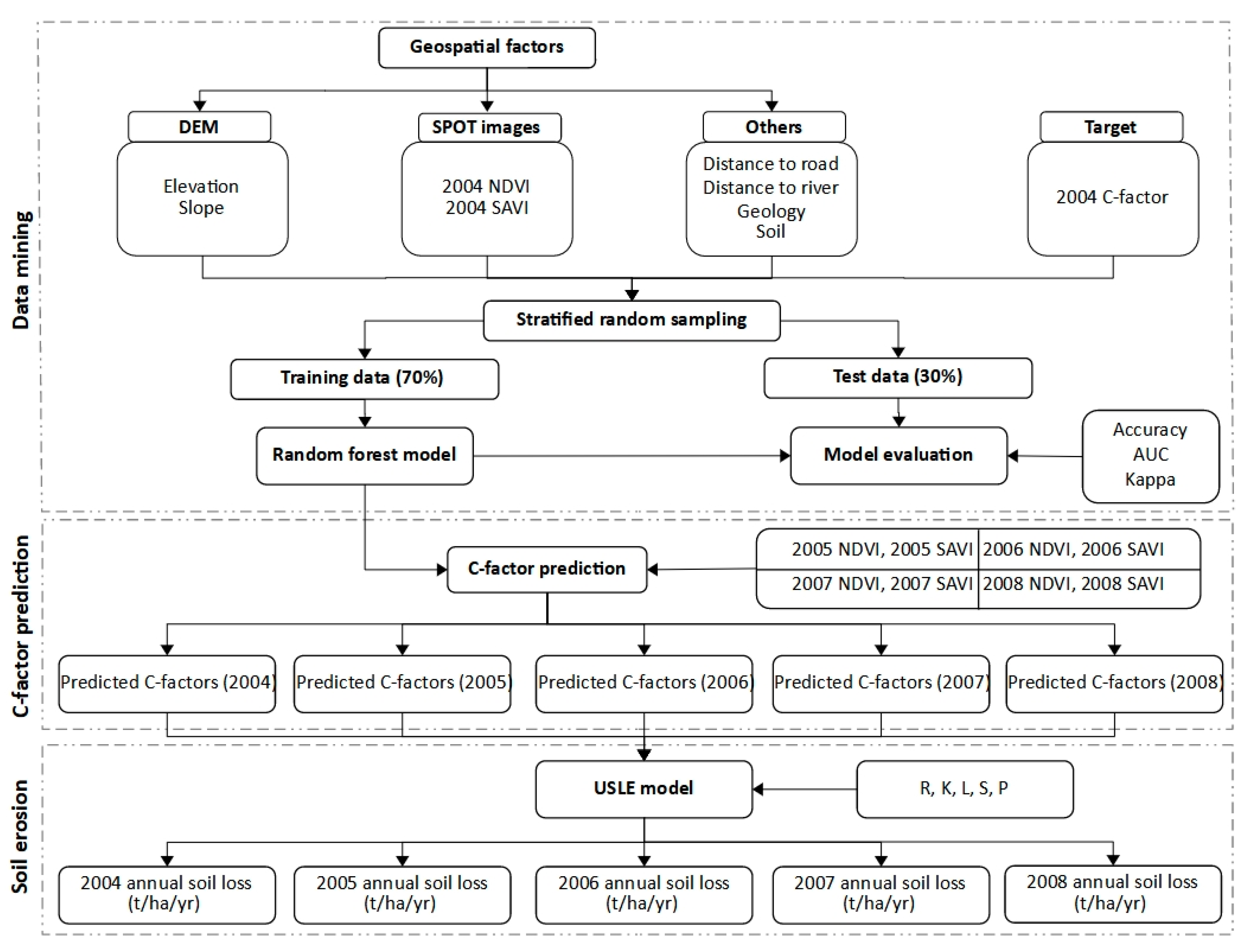
2.3. Data Mining Analysis
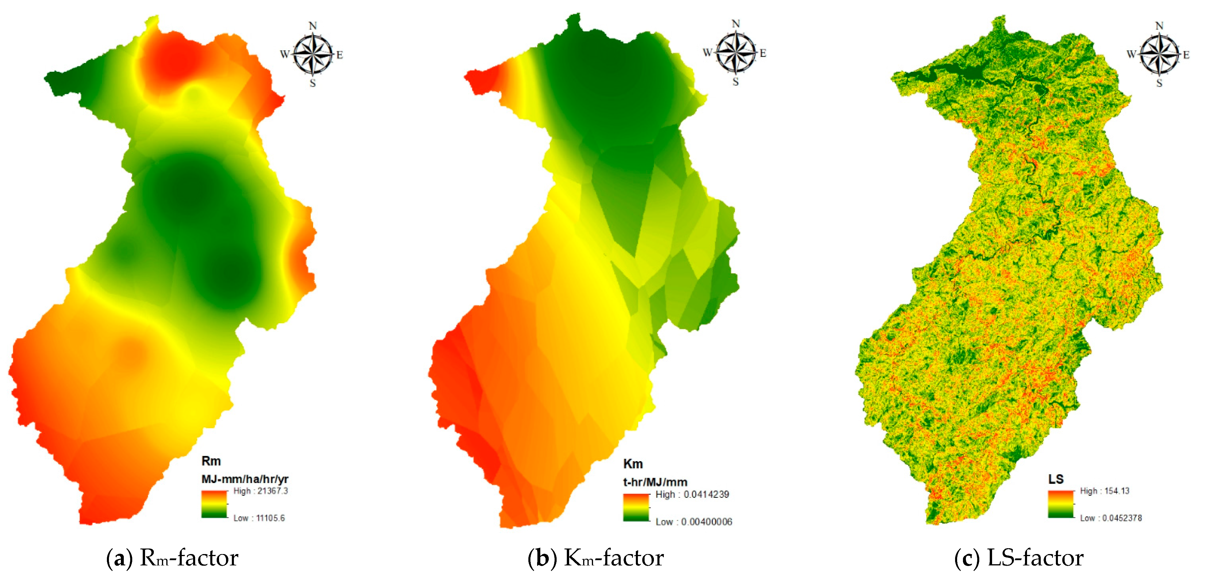
2.4. USLE Computation
3. Results and Discussion
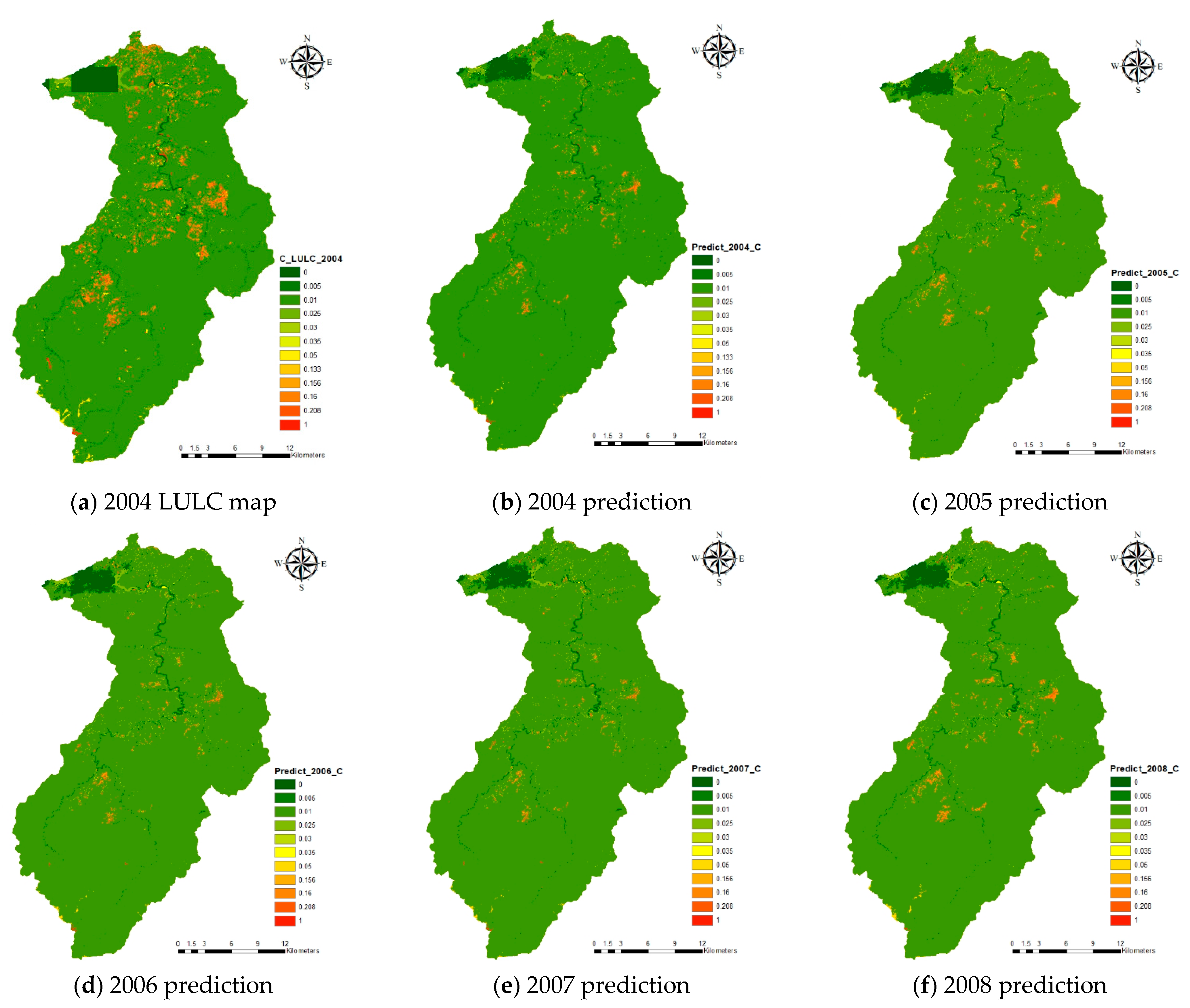
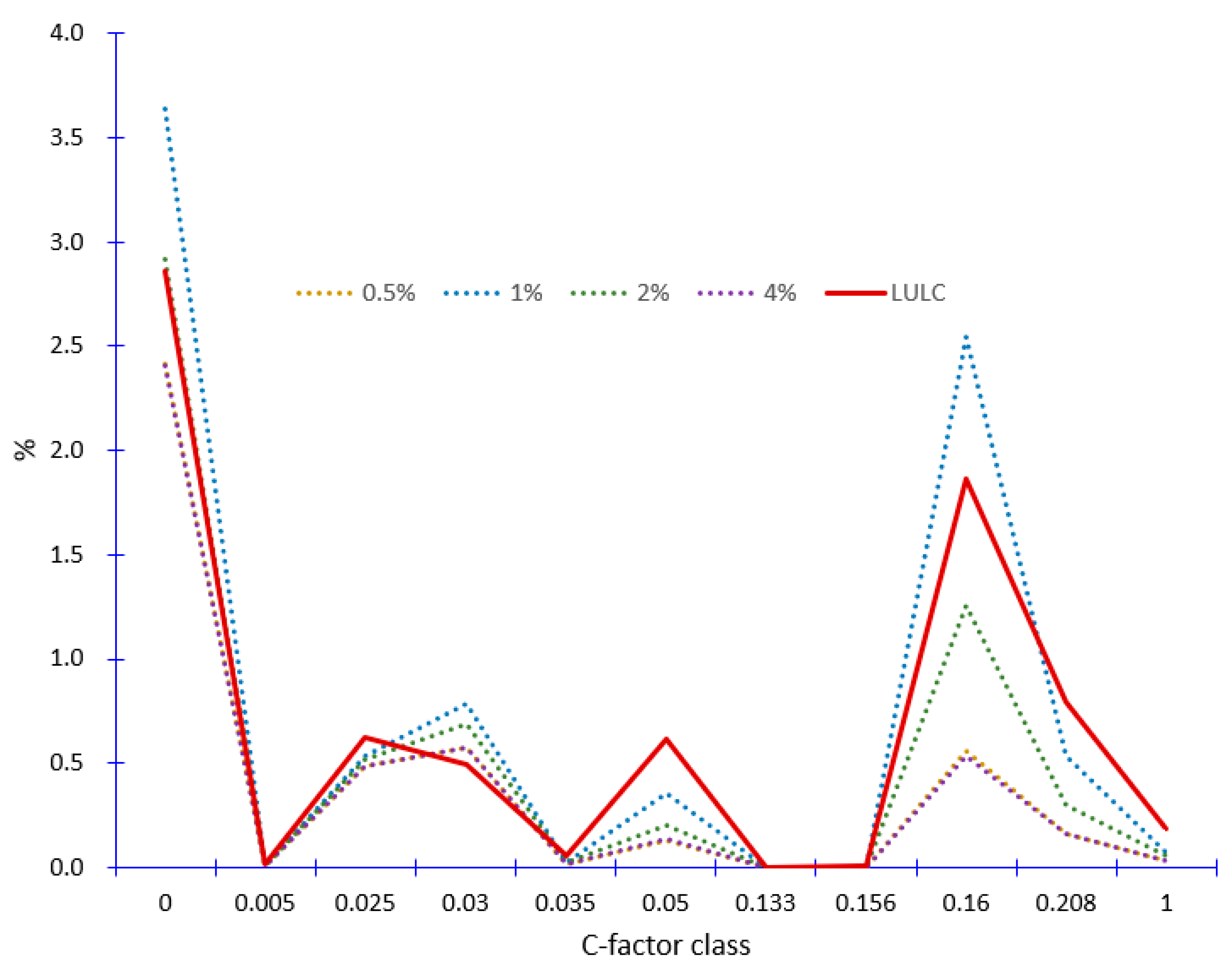
3.1. Cover-Management Factor Modeling
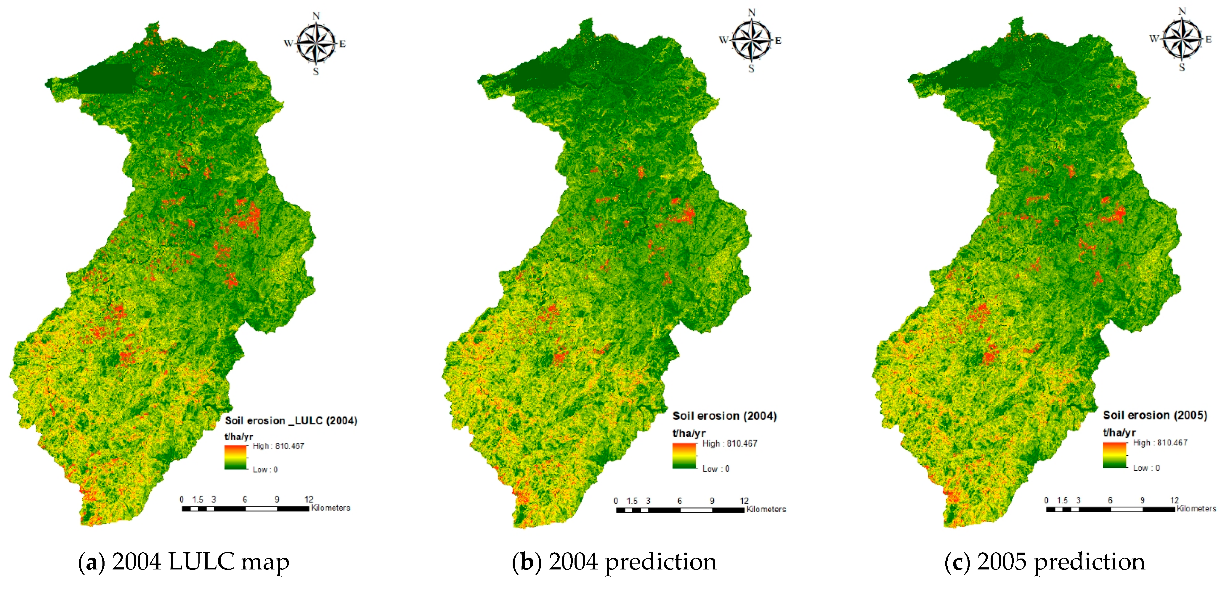
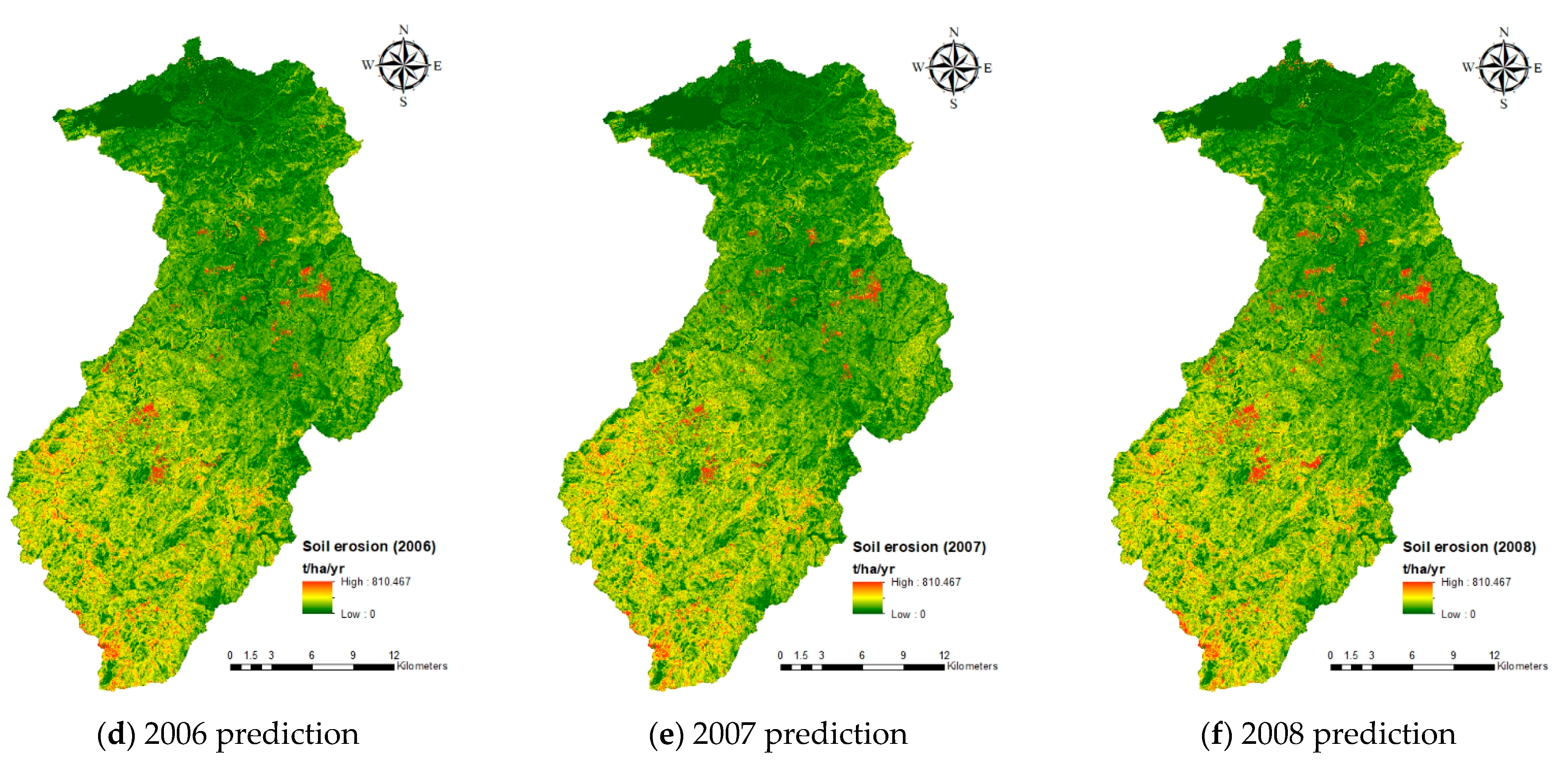
3.2. Soil Erosion Estimation
3.3. Discussion
4. Conclusions
- Overall accuracy and true positive rate of the majority class: 4%
- Kappa coefficient, AUC, and true positive rate of all minority classes combined: 0.5%
- Average C-factor: 1%
- Soil erosion rate: 2%
Author Contributions
Funding
Institutional Review Board Statement
Informed Consent Statement
Data Availability Statement
Conflicts of Interest
References
- National Research Council. Soil Conservation: Assessing the National Resources Inventory; National Academy Press: Washington, DC, USA, 1986. [Google Scholar]
- Laflen, J.M.; Moldenhauer, W.C. Pioneering Soil Erosion Prediction—The USLE Story; World Association of Soil and Water Conservation: Beijing, China, 2003. [Google Scholar]
- Young, R.A.; Onstad, C.A.; Bosch, D.D.; Anderson, W.P. Agricultural Non-Point Source Pollution Model, Version 4.03. AGNPS User’s Guide; North Central Soil Conservation Research Laboratory: Morris, MN, USA, 1994. [Google Scholar]
- Knisel, W.G. CREAMS: A Field Scale Model for Chemicals, Runoff, and Erosion from Agricultural Management Systems; U.S. Department of Agriculture, Science and Education Administration: Washington, DC, USA, 1980.
- Sharpley, A.N.; Williams, J.R. EPIC Erosion/Productivity Impact Calculator: 1. Model Documentation; U.S. Department of Agriculture, Technical Bulletin: Washington, DC, USA, 1990; Volume 1768, p. 235.
- Arnold, J.G.; Williams, J.R.; Nicks, A.D.; Sammons, N.B. SWRRB: A Basin Scale Simulation Model for Soil and Water Resources Management; Texas A&M University Press: College Station, TX, USA, 1990. [Google Scholar]
- Nearing, M.A.; Foster, G.R.; Lane, L.J.; Finkner, S.C. A process-based soil erosion model for USDA-Water Erosion Prediction Project technology. Trans. ASAE 1989, 32, 1587–1593. [Google Scholar] [CrossRef]
- Wischmeier, W.H.; Smith, D.D. Predicting Rainfall-Erosion Losses from Cropland East of the Rocky Mountains; U.S. Department of Agriculture, Agriculture Handbook: Washington, DC, USA, 1965; Volume 282, p. 49.
- Wischmeier, W.H.; Smith, D.D. Predicting Rainfall Erosion Losses—A Guide to Conservation Planning; U.S. Department of Agriculture, Agriculture Handbook: Washington, DC, USA, 1978; Volume 537, p. 67.
- Sillanpää, M. Micronutrient Assessment at the Country Level: An International Study; FAO Soils Bulletin: Rome, Italy, 1990; Volume 63, p. 214. [Google Scholar]
- Foster, G.R.; Wischmeier, W. Evaluating irregular slopes for soil loss prediction. Trans. ASAE 1974, 17, 305–309. [Google Scholar] [CrossRef]
- Griffin, M.L.; Beasley, D.B.; Fletcher, J.J.; Foster, G.R. Estimating soil loss on topographically non-uniform field and farm units. J. Soil Water Conserv. 1988, 43, 326–331. [Google Scholar]
- Renard, K.G.; Foster, G.R.; Weesies, G.A.; Porter, J.P. RUSLE: Revised Universal Soil Loss Equation. J. Soil Water Conserv. 1991, 46, 30–33. [Google Scholar]
- Chen, W.; Li, D.-H.; Yang, K.-J.; Tsai, F.; Seeboonruang, U. Identifying and comparing relatively high soil erosion sites with four DEMs. Ecol. Eng. 2018, 120, 449–463. [Google Scholar] [CrossRef]
- Li, J.-Y.; Yang, K.-J.; Chen, W. Approximation Equation of Erosion Calculation in GIS. In Proceedings of the 37th Asian Conference on Remote Sensing, Colombo, Sri Lanka, 17–21 October 2016; Volume 3, pp. 1837–1843. [Google Scholar]
- Gabriels, D.; Ghekiere, G.; Schiettecatte, W.; Rottiers, I. Assessment of USLE cover-management C-factors for 40 crop rotation systems on arable farms in the Kemmelbeek watershed, Belgium. Soil Tillage Res. 2003, 74, 47–53. [Google Scholar] [CrossRef]
- Renard, K.G.; Foster, G.R.; Weesies, G.A.; McCool, D.K.; Yoder, D.C. Predicting Soil Erosion by Water: A Guide to Conservation Planning with the Revised Universal Soil Loss Equation (RUSLE); U.S. Department of Agriculture, Agriculture Handbook: Washington, DC, USA, 1997; Volume 703, p. 404.
- Borrelli, P.; Märker, M.; Panagos, P.; Schütt, B. Modeling soil erosion and river sediment yield for an intermountain drainage basin of the Central Apennines, Italy. Catena 2014, 114, 45–58. [Google Scholar] [CrossRef]
- Dabral, P.P.; Baithuri, N.; Pandey, A. Soil erosion assessment in a hilly catchment of north eastern India using USLE, GIS and Remote Sensing. Water Resour. Manag. 2008, 22, 1783–1798. [Google Scholar] [CrossRef]
- Pandey, A.; Chowdary, V.M.; Mal, B.C. Identification of critical erosion prone areas in the small agricultural watershed using USLE, GIS and remote sensing. Water Resour. Manag. 2007, 21, 729–746. [Google Scholar] [CrossRef]
- Alexandridis, T.K.; Sotiropoulou, A.M.; Bilas, G.; Karapetsas, N.; Silleos, N.G. The effects of seasonality in estimating the C-factor of soil erosion studies. Land Degrad. Dev. 2015, 26, 596–603. [Google Scholar] [CrossRef]
- Van der Knijff, J.M.; Jones, R.J.A.; Montanarella, L. Soil Erosion Risk Assessment in Italy; European Soil Bureau: Brussels, Belgium, 1999; p. 58. [Google Scholar]
- Ayalew, D.A.; Deumlich, D.; Šarapatka, B.; Doktor, D. Quantifying the Sensitivity of NDVI-Based C Factor Estimation and Potential Soil Erosion Prediction using Spaceborne Earth Observation Data. Remote Sens. 2020, 12, 1136. [Google Scholar] [CrossRef] [Green Version]
- Tsai, F.; Lai, J.-S.; Chen, W.W.; Lin, T.-H. Analysis of topographic and vegetative factors with data mining for landslide verification. Ecol. Eng. 2013, 61, 669–677. [Google Scholar] [CrossRef]
- Tsai, F.; Chen, L.C. Long-term landcover monitoring and disaster assessment in the Shihmen reservoir watershed using satellite images. In Proceedings of the 13th CeRES International Symposium on Remote Sensing, Chiba, Japan, 29 October 2007. [Google Scholar]
- Lai, J.-S.; Tsai, F.; Lin, T.-Y.; Chen, W. Verification and susceptibility assessment for landslides using data mining techniques. J. Photogramm. Remote Sens. 2013, 17, 149–160, (In Chinese with English Abstract). [Google Scholar]
- Huete, A.R. A soil-adjusted vegetation index (SAVI). Remote Sens. Environ. 1988, 25, 295–309. [Google Scholar] [CrossRef]
- Minnaert, M. The reciprocity principle in lunar photometry. Astrophys. J. 1941, 93, 403–410. [Google Scholar] [CrossRef]
- Jhan, Y.K. Analysis of Soil Erosion of Shihmen Reservoir Watershed. Master’s Thesis, National Taipei University of Technology, Taipei, Taiwan, 2014. (In Chinese with English Abstract). [Google Scholar]
- Lin, T.-C. Establishment of Relationship between USLE Cover Management Factor and Spatial Data. Master’s Thesis, National Central University, Zhongli City, Taoyuan, Taiwan, 2016. (In Chinese with English Abstract). [Google Scholar]
- Ouyang, Y.; Luo, S.M.; Cui, L.H.; Wang, Q.; Zhang, J.E. Estimation of real-time N load in surface water using dynamic data-driven application system. Ecol. Eng. 2011, 37, 616–621. [Google Scholar] [CrossRef]
- Witten, I.H.; Frank, E.; Hall, M.A. Data Mining: Practical Machine Learning Tools and Techniques, 3rd ed.; Morgan Kaufmann: San Francisco, CA, USA, 2011. [Google Scholar]
- Breiman, L. Random forests. Mach. Learn. 2001, 45, 5–32. [Google Scholar] [CrossRef] [Green Version]
- Belgiu, M.; Dragut, L. Random forest in remote sensing: A review of applications and future directions. ISPRS J. Photogramm. Remote Sens. 2016, 114, 24–31. [Google Scholar] [CrossRef]
- Stumpf, A.; Kerle, N. Object-oriented mapping of landslides using Random Forests. Remote Sens. Environ. 2011, 115, 2564–2577. [Google Scholar] [CrossRef]
- Tsai, F.; Lai, J.-S.; Lu, Y.-H. Full-waveform LiDAR point cloud land cover classification with volumetric texture measures. Terr. Atmos. Ocean. Sci. 2016, 27, 549–563. [Google Scholar] [CrossRef] [Green Version]
- Nguyen, K.A.; Chen, W.; Lin, B.-S.; Seeboonruang, U.; Thomas, K. Predicting sheet and rill erosion of Shihmen reservoir watershed in Taiwan using machine learning. Sustainability 2019, 11, 3615. [Google Scholar] [CrossRef] [Green Version]
- Ismail, R.; Mutanga, O.; Kumar, L. Modeling the potential distribution of pine forests susceptible to Sirex Noctilio infestations in Mpumalang, South African. Trans. GIS 2010, 14, 709–726. [Google Scholar] [CrossRef]
- Guo, L.; Chehata, N.; Mallet, C.; Boukir, S. Relevance of airborne LiDAR and multispectral image data for urban scene classification using random forests. ISPRS J. Photogramm. Remote Sens. 2011, 66, 56–66. [Google Scholar] [CrossRef]
- Zhang, F.; Yang, X. Improving land cover classification in an urbanized coastal area by random forests: The role of variable selection. Remote Sens. Environ. 2020, 251, 112105. [Google Scholar] [CrossRef]
- Han, J.; Kamber, M.; Pei, J. Data Mining, Concepts and Techniques, 3rd ed.; Morgan Kaufmann: Waltham, MA, USA, 2012. [Google Scholar]
- Liu, Y.-H.; Li, D.-H.; Chen, W.; Lin, B.-S.; Seeboonruang, U.; Tsai, F. Soil erosion modeling and comparison using slope units and grid cells in Shihmen reservoir watershed in Northern Taiwan. Water 2018, 10, 1387. [Google Scholar] [CrossRef] [Green Version]
- Lin, W.Y.; Lin, L.L. Application and discussion of soil erosion prediction model. J. Soil Water Conserv. 2008, 40, 357–368, (In Chinese with English Abstract). [Google Scholar]
- Lin, B.S.; Thomas, K.; Chen, C.K.; Ho, H.C. Evaluation of soil erosion risk for watershed management in Shenmu watershed, central Taiwan using USLE model parameters. Paddy Water Environ. 2008, 14, 19–43. [Google Scholar] [CrossRef]
- Li, D.-H. Analyzing Soil Erosion of Shihmen Reservoir Watershed Using Slope Units. Master’s Thesis, National Taipei University of Technology, Taipei, Taiwan, 2017. (In Chinese with English Abstract). [Google Scholar]


| Approach | Method | Advantage | Challenge | |
|---|---|---|---|---|
| 1 | LULC map by field survey |
| Most accurate LULC data | Time-consuming with a lengthy update period |
| 2 | LULC map by remote sensing |
| Multi-temporal evaluation | Ground truthing needed to ensure accuracy |
| 3 | Empirical NDVI equation |
| Simple and multi-temporal evaluation | Sensitive to vegetation phenology and soil conditions |
| 4 | This study |
| More accurate model and multi-temporal evaluation | More complicated |
| Original Data | Derived Data | Note |
|---|---|---|
| DEM | Elevation (numeric) | Cell size: 10 m |
| Slope (numeric) | ||
| SPOT satellite images | NDVI (numeric) | See Table 3 for details |
| SAVI (numeric) | ||
| Road map | Distance to road (numeric) | Measurement unit: meter |
| Stream map | Distance to river (numeric) | |
| Geology map | Geological formation (categorical) |
|
| Soil map | Soil type (categorical) |
|
| Sensor | Date | Spatial Resolution (m) | Spectral Bandwidth (um) | Radiometric Resolution (bits) |
|---|---|---|---|---|
| SPOT 5 | 2004/10/12 | 10 | Green: 0.50–0.59 Red: 0.61–0.68 NIR: 0.79–0.89 | 8 |
| 2006/07/19 | ||||
| 2008/09/21 | ||||
| SPOT 4 | 2005/07/25 | 20 | ||
| 2007/07/19 |
| C-Factor Class | Land Use/Land Cover Class |
|---|---|
| 0 | Waterbody, reef |
| 0.005 | Railway related facility, weir, dam, cultural facility |
| 0.01 | Natural forest, artificial forest, residential area |
| 0.025 | Dike, ditch, aqueduct, shoal, beach, wetland |
| 0.03 | Provincial road, road |
| 0.035 | Unused land, land being converted |
| 0.05 | Pastureland, logging land, grassland, shrubland |
| 0.133 | Livestock house |
| 0.156 | Abandoned farmland |
| 0.16 | Orchard |
| 0.208 | Dry-farming land |
| 1 | Fire break, bare land |
| No. | C-factor Class | Total no. of Points (Population) | 4% of the Majority Class | 2% of the Majority Class | 1% of the Majority Class | 0.5% of the Majority Class |
|---|---|---|---|---|---|---|
| % of the Total Sample (Input Dataset) | ||||||
| 1 | 0 | 216,970 | 8679 (2.9%) | 8679 (5.3%) | 8679 (9.3%) | 8679 (15.0%) |
| 2 | 0.005 | 1110 | 44 (0.0%) | 44 (0.0%) | 44 (0.0%) | 44 (0.1%) |
| 3 | 0.01 | 7,021,560 | 280,862 (92.5%) | 140,431 (86.0%) | 70,216 (75.5%) | 35,108 (60.6%) |
| 4 | 0.025 | 47,629 | 1905 (0.6%) | 1905 (1.2%) | 1905 (2.0%) | 1905 (3.3%) |
| 5 | 0.03 | 37,714 | 1509 (0.5%) | 1509 (0.9%) | 1509 (1.6%) | 1509 (2.6%) |
| 6 | 0.035 | 4235 | 169 (0.1%) | 169 (0.1%) | 169 (0.2%) | 169 (0.3%) |
| 7 | 0.05 | 46,598 | 1864 (0.6%) | 1864 (1.1%) | 1864 (2.0%) | 1864 (3.2%) |
| 8 | 0.133 | 73 | 3 (0.0%) | 3 (0.0%) | 3 (0.0%) | 3 (0.0%) |
| 9 | 0.156 | 342 | 14 (0.0%) | 14 (0.0%) | 14 (0.0%) | 14 (0.0%) |
| 10 | 0.16 | 141,672 | 5667 (1.9%) | 5667 (3.5%) | 5667 (6.1%) | 5667 (9.8%) |
| 11 | 0.208 | 60,060 | 2402 (0.8%) | 2402 (1.5%) | 2402 (2.6%) | 2402 (4.1%) |
| 12 | 1 | 14,099 | 564 (0.2%) | 564 (0.3%) | 564 (0.6%) | 564 (1.0%) |
| Total | 7,592,062 | 100.0% | 100.0% | 100.0% | 100.0% | |
| Symbol | Definition | Unit |
|---|---|---|
| Am | Average annual soil loss | t/ha-year |
| Rm | Rainfall erosivity factor | MJ-mm/ha-hour-year |
| Km | Soil erodibility factor | t-hour/MJ-mm |
| L | Slope length factor | -- |
| S | Slope steepness factor | -- |
| C | Cover management factor | -- |
| P | Support practice factor | -- |
| Actual | Predicted | |||||||||||
|---|---|---|---|---|---|---|---|---|---|---|---|---|
| 0 | 0.005 | 0.01 | 0.025 | 0.03 | 0.035 | 0.05 | 0.133 | 0.156 | 0.16 | 0.208 | 1 | |
| 0 | 1792 | 0 | 732 | 75 | 1 | 0 | 1 | 0 | 0 | 3 | 0 | 0 |
| 0.005 | 0 | 3 | 8 | 0 | 0 | 0 | 2 | 0 | 0 | 0 | 0 | 0 |
| 0.01 | 249 | 0 | 83,729 | 7 | 130 | 1 | 19 | 0 | 0 | 101 | 19 | 4 |
| 0.025 | 109 | 0 | 89 | 372 | 0 | 0 | 1 | 0 | 0 | 0 | 0 | 0 |
| 0.03 | 2 | 0 | 99 | 0 | 349 | 0 | 0 | 0 | 0 | 2 | 1 | 0 |
| 0.035 | 2 | 0 | 32 | 3 | 3 | 8 | 0 | 0 | 0 | 2 | 1 | 0 |
| 0.05 | 13 | 0 | 441 | 4 | 8 | 0 | 85 | 0 | 0 | 7 | 1 | 0 |
| 0.133 | 0 | 0 | 1 | 0 | 0 | 0 | 0 | 0 | 0 | 0 | 0 | 0 |
| 0.156 | 0 | 0 | 4 | 0 | 0 | 0 | 0 | 0 | 0 | 0 | 0 | 0 |
| 0.16 | 6 | 0 | 1400 | 0 | 24 | 0 | 0 | 0 | 0 | 251 | 19 | 0 |
| 0.208 | 5 | 0 | 559 | 0 | 17 | 1 | 0 | 0 | 0 | 58 | 81 | 0 |
| 1 | 1 | 0 | 133 | 7 | 2 | 0 | 0 | 0 | 0 | 1 | 0 | 25 |
| Overall statistics | OA = 0.952 | Kappa = 0.574 | AUC = 0.780 | |||||||||
| Official LULC Map (Mean) | RF Model Prediction (Mean) | |||||
|---|---|---|---|---|---|---|
| 2004 | 2004 | 2005 | 2006 | 2007 | 2008 | |
| 4% | 0.0164 | 0.0115 | 0.0114 | 0.0110 | 0.0110 | 0.0115 |
| 2% | 0.0130 | 0.0132 | 0.0125 | 0.0124 | 0.0133 | |
| 1% | 0.0156 | 0.0164 | 0.0149 | 0.0146 | 0.0169 | |
| 0.5% | 0.0115 | 0.0114 | 0.0110 | 0.0109 | 0.0115 | |
| Actual | Predicted | |||||||||||
|---|---|---|---|---|---|---|---|---|---|---|---|---|
| 0 | 0.005 | 0.01 | 0.025 | 0.03 | 0.035 | 0.05 | 0.133 | 0.156 | 0.16 | 0.208 | 1 | |
| 0 | 2034 | 0 | 494 | 62 | 0 | 0 | 3 | 0 | 0 | 4 | 6 | 1 |
| 0.005 | 0 | 6 | 5 | 0 | 0 | 0 | 2 | 0 | 0 | 0 | 0 | 0 |
| 0.01 | 234 | 0 | 41,551 | 4 | 83 | 1 | 21 | 0 | 0 | 188 | 41 | 6 |
| 0.025 | 113 | 0 | 85 | 371 | 1 | 0 | 1 | 0 | 0 | 0 | 0 | 0 |
| 0.03 | 1 | 0 | 37 | 0 | 401 | 4 | 0 | 0 | 0 | 9 | 1 | 0 |
| 0.035 | 1 | 0 | 20 | 1 | 1 | 15 | 0 | 0 | 0 | 8 | 5 | 0 |
| 0.05 | 10 | 1 | 402 | 5 | 2 | 0 | 124 | 0 | 0 | 11 | 4 | 0 |
| 0.133 | 0 | 0 | 1 | 0 | 0 | 0 | 0 | 0 | 0 | 0 | 0 | 0 |
| 0.156 | 0 | 0 | 4 | 0 | 0 | 0 | 0 | 0 | 0 | 0 | 0 | 0 |
| 0.16 | 7 | 0 | 1095 | 0 | 24 | 0 | 0 | 0 | 0 | 540 | 34 | 0 |
| 0.208 | 9 | 0 | 440 | 0 | 19 | 0 | 0 | 0 | 0 | 123 | 130 | 0 |
| 1 | 2 | 0 | 130 | 2 | 0 | 0 | 0 | 0 | 0 | 2 | 1 | 32 |
| Overall statistics | OA = 0.923 | Kappa = 0.648 | AUC = 0.781 | |||||||||
| Official LULC Map (2004) | RF Model Prediction | Erosion Pins (2008–2011) | ||||||
|---|---|---|---|---|---|---|---|---|
| 2004 | 2005 | 2006 | 2007 | 2008 | ||||
| Am (t/ha-year) | 116.3 | 88.2 | 85.6 | 84.7 | 84.0 | 84.5 | (4% of C = 0.01) | 90.6 |
| 95.1 | 94.4 | 92.4 | 91.6 | 93.2 | (2% of C = 0.01) | |||
| Sampling Rate of the Majority Class | OA | Kappa | AUC | True Positive Rate of All Minority Classes Combined | True Positive Rate of the Majority Class | Average C-Factor of LULC Map | Average C-Factor (2004) | Soil Erosion of 2004 (t/ha-Year) | Soil Erosion of 2008 (t/ha-Year) | Erosion Pins (2008–2011) |
|---|---|---|---|---|---|---|---|---|---|---|
| 4% | 0.952 | 0.574 | 0.780 | 0.43 | 0.99 | 0.0164 | 0.0115 | 88.2 | 84.5 | 90.6 |
| 2% | 0.923 | 0.648 | 0.781 | 0.53 | 0.99 | 0.0130 | 95.1 | 93.2 | ||
| 1% | 0.880 | 0.687 | 0.845 | 0.61 | 0.97 | 0.0156 | 104.3 | 108.0 | ||
| 0.5% | 0.846 | 0.732 | 0.891 | 0.70 | 0.94 | 0.0115 | 88.2 | 84.5 |
Publisher’s Note: MDPI stays neutral with regard to jurisdictional claims in published maps and institutional affiliations. |
© 2021 by the authors. Licensee MDPI, Basel, Switzerland. This article is an open access article distributed under the terms and conditions of the Creative Commons Attribution (CC BY) license (http://creativecommons.org/licenses/by/4.0/).
Share and Cite
Tsai, F.; Lai, J.-S.; Nguyen, K.A.; Chen, W. Determining Cover Management Factor with Remote Sensing and Spatial Analysis for Improving Long-Term Soil Loss Estimation in Watersheds. ISPRS Int. J. Geo-Inf. 2021, 10, 19. https://doi.org/10.3390/ijgi10010019
Tsai F, Lai J-S, Nguyen KA, Chen W. Determining Cover Management Factor with Remote Sensing and Spatial Analysis for Improving Long-Term Soil Loss Estimation in Watersheds. ISPRS International Journal of Geo-Information. 2021; 10(1):19. https://doi.org/10.3390/ijgi10010019
Chicago/Turabian StyleTsai, Fuan, Jhe-Syuan Lai, Kieu Anh Nguyen, and Walter Chen. 2021. "Determining Cover Management Factor with Remote Sensing and Spatial Analysis for Improving Long-Term Soil Loss Estimation in Watersheds" ISPRS International Journal of Geo-Information 10, no. 1: 19. https://doi.org/10.3390/ijgi10010019