Detection of False Synchronization of Stereo Image Transmission Using a Convolutional Neural Network


Faculty of Mechanical Engineering and Computer Science, Department of Computer Science, Czestochowa University of Technology, Dabrowskiego 73, 42-201 Czestochowa, Poland
*
Author to whom correspondence should be addressed.
Symmetry 2021, 13(1), 78; https://doi.org/10.3390/sym13010078
Submission received: 14 December 2020
/
Revised: 30 December 2020
/
Accepted: 2 January 2021
/
Published: 5 January 2021
Abstract
:The subject of the work described in this article is the detection of false synchronization in the transmission of digital stereo images. Until now, the synchronization problem was solved by using start triggers in the recording. Our proposal checks the discrepancy between the received pairs of images, which allows you to detect delays in transferring images between the left camera and the right camera. For this purpose, a deep network is used to classify the analyzed pairs of images into five classes: MuchFaster, Faster, Regular, Slower, and MuchSlower. As can be seen as a result of the conducted work, satisfactory research results were obtained as the correct classification. A high percentage of average probability in individual classes also indicates a high degree of certainty as to the correctness of the results. An author’s base of colorful stereo images in the number of 3070 pairs is used for the research.
1. Introduction
Mobile robots have been a very popular topic in the last decade [1,2,3]. Their operation is associated with simultaneous localization and mapping (SLAM) methods. Depending on the type of sensors involved, SLAM is mainly divided into 2D laser SLAM [4,5], and 3D vision SLAM [6]. Although a lot of research has been done on the system with laser sensors, there are still big problems with the three-dimensional structure of information on the environment [7] as opposed to vision-based systems.
The operations of processing and analyzing digital images provide a large amount of information about the objects located on them and their immediate surroundings. Nowadays, these processes are used in many areas of life. Stereo-vision is an important part of image research, especially in situations where information about space, the surroundings of the object in the image, or its location is more important than information about the object itself. A lot of research is being carried out in this topics, such as 3D scene reconstruction [8,9], depth detection [10], or autonomous navigation of unmanned vehicles in environments without GPS [11]. Stereo-vision is also used as work validation [12]. The work on stereo-vision consists of the analysis and processing of digital images obtained from two or more than two digital cameras (multi-vision stereo) [13,14,15].
Working with stereo streams provides more information than a single image of the same scene. Disturbances such as distortion [16], noise, or lack of sharpness are an obvious problem. Unfortunately, there are also problems in stereo-vision that are not found in the analysis of individual digital images, such as the need to calibrate cameras [17,18]. The essence of stereo-vision is the recording of images of the same scene from two different observation points, made in identical conditions. In addition, video stream recording must be done at the same time.
There are three main reasons for incorrect stereo image analysis results. The first is errors in the calibration of the research stand or the calibration of the cameras themselves [17,18]. The second is errors in the program, in the implementation of algorithms for processing and analyzing digital images. The third one is false synchronization in data transmission from both cameras. The first two types of errors most often occur as a result of human error and are characterized by repeatability under similar conditions. The third type of error may appear unexpectedly. Often, in the course of multiple analyses carried out even on the same configured test stand, a series of correct results is obtained. Which may suggest that the results obtained in subsequent analyses will be correct and the results obtained may be incorrect. The reason is the lack of data transfer synchronization. Such errors may be undetected or detected but too late.
A car traveling at a speed of 50 km/h moves by 13.89 m in 1 s; if it is recorded by two cameras with a recording frequency of 30 frames per second, then its distance changes between subsequent frames by 0.463 m. Therefore, a delay in the image transmission between cameras by at least one frame returns incorrect information. The delay of half a second is close to 7 m difference in the distance between the recording of the first and second cameras. This is a very serious problem in the analysis of stereo images, so it is very important to introduce additional operations for the rapid detection of such errors. The use of classification as a detection method gives very good results. This is a popular way in many areas such as fake news [19,20], for objects defects detection [21], used for medical images [22,23] and recognition of human speech [24,25].
The problem of camera synchronization is often overlooked, mainly because the research uses devices with built-in camera sets, which are equipped with starting systems, and the output data is one signal containing the recorded image from all cameras simultaneously. It is a very practical solution, although it introduces an additional measurement error (resulting from the operation of a given device). Such devices are many times more expensive than systems consisting of several separate cameras.
In the sets of several cameras being separate devices, several separate signals are obtained. Such sets must be properly synchronized when starting and transmitting the result signals. Such a stand gives greater possibilities in the controllability or repairs of individual devices, which, depending on the purpose of the work, maybe crucial.
The subject of the work described in the article was the detection of false synchronization in the transmission of digital stereo images, assuming that the test bench consists of a set of separate, inexpensive devices. For this purpose, a deep web was used to classify the analyzed image pairs into five classes: MuchFaster, Faster, Regular, Slower, and MuchSlower.
2. Stereo-Vision
As mentioned earlier, at least two digital images are analyzed in stereo-vision. Research on two images is the most common so far and it is called a pair of images [17,18]. Usually, it is a pair consisting of the left image and the right image.
It is obvious that it cannot be a pair of any two images, but they must be properly taken images. Photographs recorded from two cameras located at a certain distance from the recorded scene and located at a small distance from each other will allow obtaining two images of the same scene but with some differences.
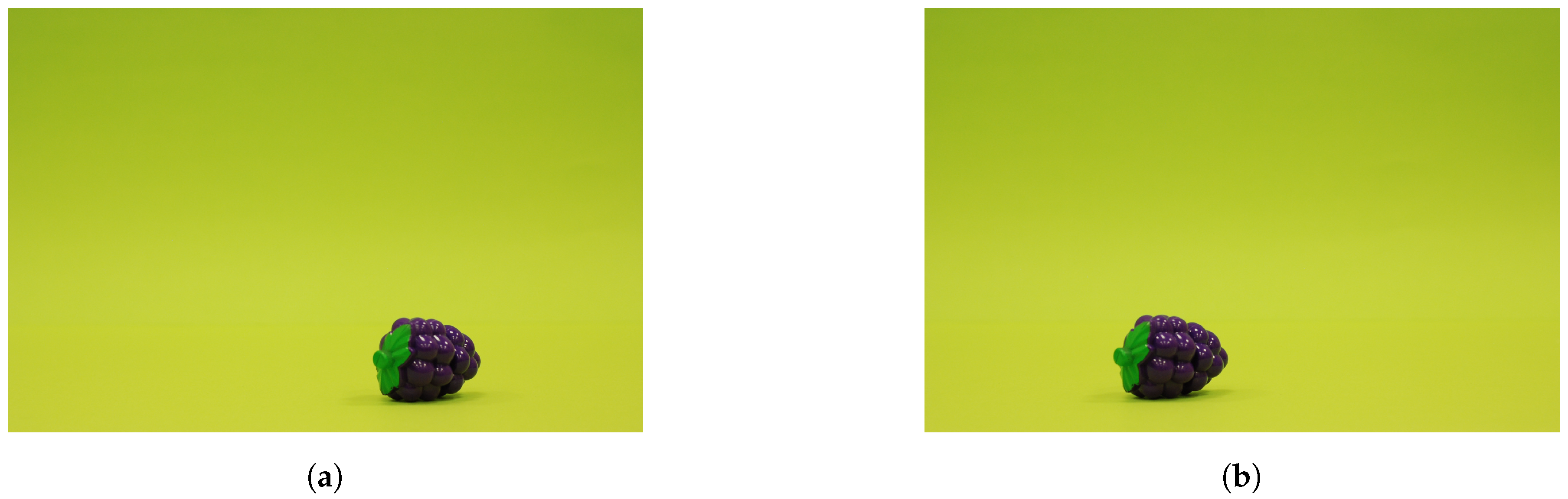
As shown in Figure 1 the image from the right camera will be slightly shifted relative to the image from the left camera, and the objects on the stage will be recorded at a slightly different angle. Analyzing these differences is the foundation of all stereo-vision research [18].
To obtain a pair of images suitable for analysis, they should be taken under appropriate conditions. The first thing to do is calibrate the test stand. The second is camera synchronization. Images must be taken by cameras with the same parameters, such as focal length. Images should also have the same resolution. It is also important that they are recorded in the same lighting conditions.
Taking appropriate pairs of images as individual images can be done even with one digital camera. After taking the first image, the camera is moved, and then the second image is taken, taking into account all parameters. Of course, this is only possible when registering static objects. However, if the objects being registered are in motion, it is necessary to use two recording devices, either digital images or video streams. It is important in this case to make both recordings (corresponding images) should be done at the same time.
When analyzing stereo images in real-time, there may be a delay in sending frames (images) for analysis. If there is no synchronization in data transmission from the left camera relative to the transmission from the right camera, then we will get incorrect results from the analysis of such mismatched pairs of images. Lack of synchronization can be very dangerous, for example when recording an approaching vehicle as mentioned in the introduction.
3. Database
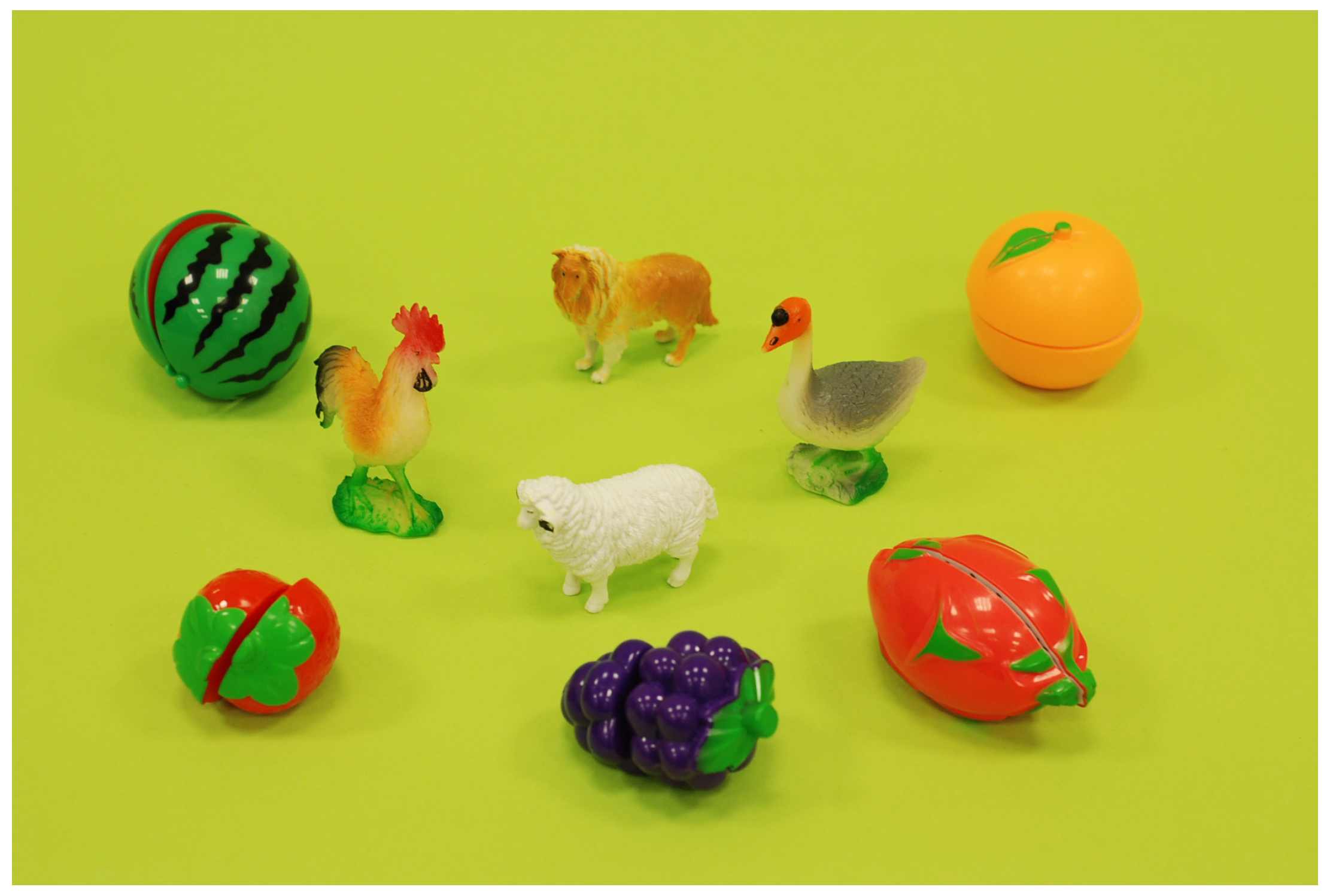
There are many digital image databases available for research purposes, but there are great difficulties accessing stereo image databases. Therefore, the 3070 pairs of images were taken, constituting the input database for this study. The images were taken with a Nikon D80 digital camera with a fixed focal length 50mm lens. The cameras were placed parallel to the photographed scene, which facilitated the spatial calibration of the test stand. One distance of 100 mm was used between the camera taking the left image and the camera taking the right image. Static objects were recorded at different distances from the lens, ranging from 800 mm to 2600 mm. The object was placed both in the central part of the photographed scene, as well as in its lateral, lower, and upper parts. This was deliberate and aimed at ensuring reality. All images were prepared in RGB format and with a resolution of 1936 × 1296 pixels. Figure 2 presents a set of photographed objects. There was always one colorful object on the photographed stage.
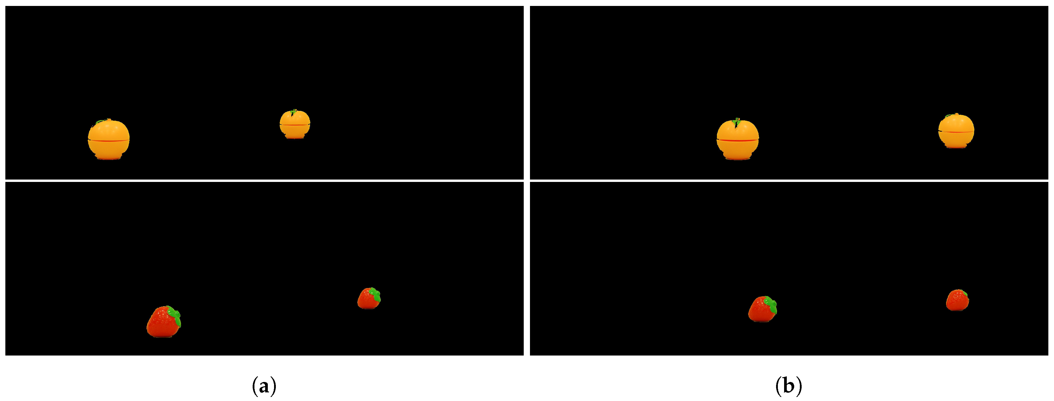
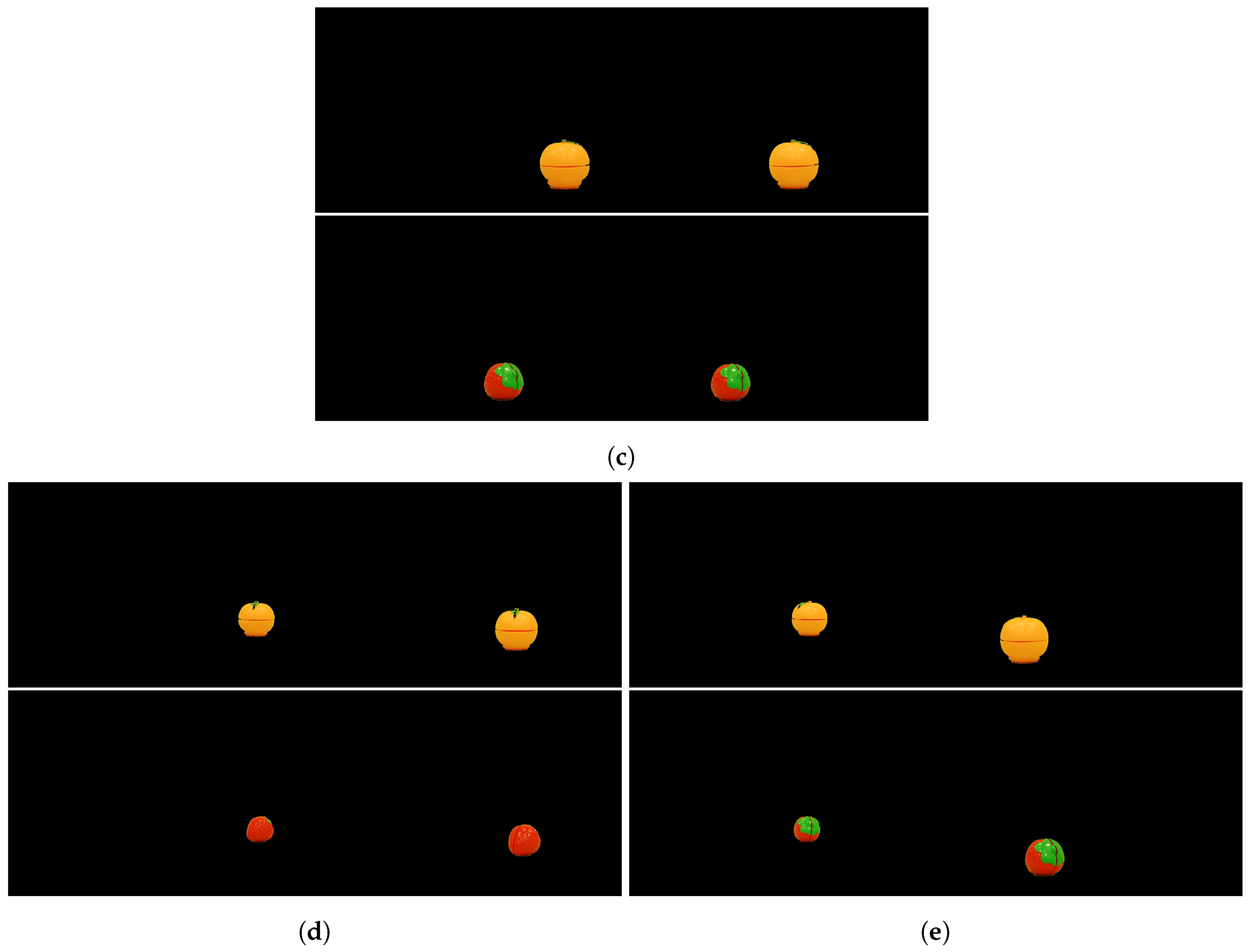
For each image, a preliminary operation was carried out involving the replacement of the entire background except the object for black. This was to exclude interference in the background color. The same object was always on the pairs of images.
It was assumed that the object was moved towards the camera, the object could be in rotational motion, and that the initial position of the object was consistent with the left image. That is why five cases arose:
- the first-named MuchSlower, when the object in the right image was much further from the lens than the object in the left image,
- the second called Slower, when the object in the right image was further from the lens than the object in the left image,
- the third called Regular when the object in the right image was at the same distance from the lens as the object in the left image,
- the fourth named Faster when the object in the right image was slightly closer to the lens than the object in the left image,
- the fifth named MuchFaster, when the object in the right image was much closer to the lens than the object in the left image.
4. Convolutional Neural Network
Convolutional Neural Networks (CNNs) [26,27] are very popular. They are part of Deep Learning and come from Artificial Neural Networks (ANNs) well known in the last century. Like any Artificial Intelligence (AI) network model, CNN is made up of layers. They are arranged in a hierarchical manner. The most important and most frequently used are Input Layer (IL), Convolution Layer (CL) [26,28], Full Connected Layer (FCL) [27,29], and Output Layer (OL). The first layer of any network is always the IL, which is used to enter data into the model. CNN is often used to deal with image data. In this case, one sample entered into the network model is one image. The whole picture is divided into receptive fields. The size of the fields depends on the size and number of filters (sometimes called masks) in the next layer set by the designer. In the next section, there is at least one CL. The CL is built of a set of neurons in which the operation of convolution of the entered data values in the scope of the receptive field with a set of filters is performed. Each filter in turn is a set of weight values. In the CL, the weights are shared. Depending on the model and its purpose, there may be a few, a dozen, or many more CLs, the only limitation is the computational capabilities of computer hardware. The task of the CLs is to learning the model and the characteristic features of the learning data. Later in the CNN model, there are FCLs, whose task is to combine the data that the network learned in the previous layers. The final layer of the network model is the OL, returning the result of the network model.
In addition to the basic CNN layers mentioned above, they also have so-called intermediate layers. These include the classic Rectified Linear Units Layer (ReLU) [26,29], often appearing immediately after the weave layer. Its job is to remove negative values. Layers such as Max or Average Pooling Layer (Max PL, Average PL) [28,29], in turn, reduce the dimensionality of successive layers. This is done by selecting the maximum or average value in a given area. Normalization layers [30] such as the Cross Channel Normalization Layer (CCNL) are also used. Another type of intermediate layer is the Dropout Layer (DL) [29], which discards randomly selected data, reducing the risk of overfitting the model. Classifying networks often use Softmax Layer (SL) [27] just before Classification Output Layer (COL) [30], which together returns the results of the model training process.
In digital image analysis, the convolution operation is commonly used to filter the image. Thanks to it, features characteristic of a given image are obtained. This is why CNNs are used with great success in studies where images are the samples in the database.
5. Research
In this article, we present a proposal to detect false synchronization of image transmission from two cameras. The two stereo-pair images have minor differences, which of course are used for e.g., searching for depth in the recorded scene, or for determining the position of individual objects and many other issues. Our observations show that if a stereo recording of images is performed in accordance with the laws of the canonical system, then such a pair of images also have common features. The first one is the almost identical size of the registered object in the left and right image. Another common feature is the position of the object in the image. For example, if in one of the images the object is higher than in the other image, it means that the object was registered at a different distance from the lens. With such observations in mind, a CNN implementation was developed, the task of which is to classify the entered pairs of images into one of five classes: MuchSlower, Slower, Regular, Faster, MuchFaster.
5.1. Convolutional Neural Network Structure
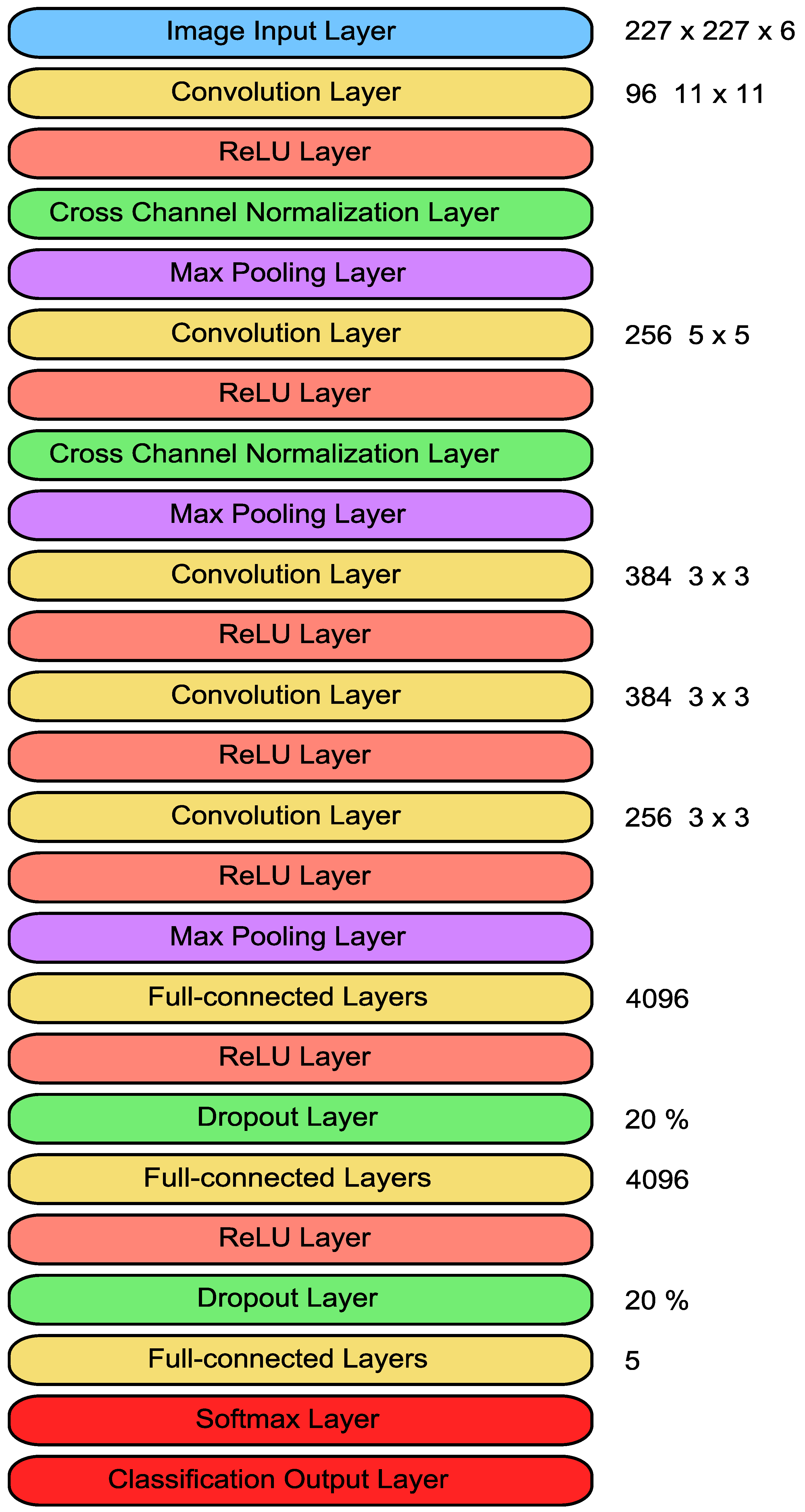
The network used for the described research consisted of 25 layers. The first is the image IL (227 × 227 × 6). In order to encode information about the introduced images, five layers of weave and three FCLs were used. A detailed diagram of the layered architecture is shown in Figure 4. It is obvious that intermediate layers such as ReLU Layer, Max PL, CCNL, which are commonly known, must also be used.
After the first CL, which has 96 11 × 11 filters, with [4 4] stride and [0 0 0 0] padding, there are three intermediate layers: ReLU, CCNL, and Max PL. As is commonly known, the tint levels of the individual colors (RGB) in the image are positive values. If the value of all colors of a pixel is equal to zero, it is black. The maximum value equal to 1 for each of the color components means white. The intermediate values are correspondingly colored pixels. As we know, the result of the convolution operation may be valued beyond the range <0, 1>, therefore the ReLU Layer was used in the first place, which converts negative values to zero. The CCNL normalizes the calculation results to values within a given range. The Max PL selects the maximum values, its window size is 3 × 3 with an offset [2 2] and padding [0 0 0 0] step. It is aim is to preserve the most important values and reduce dimensions. The next one is the second CL, which has 256 5 × 5 filters, with [1 1] stride, and [2 2 2 2] padding. Here, too, a block of layers was used: ReLU, CCNL, and Max PL, with the same parameters as above.
Then three blocks consisting of two layers: CL and ReLU were used. The CLs had filters with the size of 3 × 3, the shift by [1 1] stride and [1 1 1 1] padding, while the numbers of their filter sets were respectively 384, 384, 256. Immediately after them, one layer of Max PL with a 3 × 3 window was applied, with [2 2] stride and [0 0 0 0] padding. The use of CLs made it possible to learn the network model of the characteristics of a pair of digital images. The first convolutions look for small key elements in the images, while the subsequent CLs, along with the reduction of the dimensionality and the increasing range of the receptive field, learn the characteristics of larger elements.
Later in the model, three FCLs and two ReLU layers were used, whose task was to collect and combine information obtained from convolutional blocks. To avoid over-fitting the network, a DL with a dropout threshold of 20% was applied before the second and third FCLs.
As it is a classification network, it was obvious to use a set of three layers: FCL, SL, and COL as the last layers of the network model, this model returns five possible outputs.
5.2. Input Data
The previously presented image database was used for these studies. The entire data set of 3070 image pairs has been randomly divided into three sets: Train—60% of the entire base, Validation—20% of the whole base, and Test—20% of the whole base. Thus, the number of individual collections is respectively: Train—1840 samples, Validation—615 samples, and Test—615 samples. Then the resulting collections were converted into tensors. Each image before loading into the tensor has been converted to the matrix, scaled to 227 × 227 × 3, and double type.
All three resulting tensors had the same structure, which was as follows . The matrix for is the first image from the introduced stereo pair (image from the left camera), and the matrix for is the second image of this pairs (image from the right camera). Whereas are the consecutive numbers of the entered pairs of images.
5.3. Learning Process
Research works were carried out in the Matlab environment. CNN was developed on a computer with the following parameters: Windows 10, Intel (R) Core (TM) i7-9700K CPU @ 3.60 GHz processor, 32 GB RAM installed, NVIDIA GeForce RTX 2080 graphics card. The stochastic gradient descent with momentum (SGDM) optimizer [30] was used as the input argument. The network learning process was carried out for 150 epochs. As one training sample in the presented network model is 309,174 numerical values (227 × 227 × 6), it was necessary to set a relatively small Mini Batch Size equal to 23. This value also ensured that each database sample was used, and thus there were 80 iterations per epoch. In each epoch of learning a network model, each sample belonging to the training set was used once. Between epochs, the set of weight values obtained in the preceding epoch was verified. The entire training set was then shuffled so that each sample was independent of other samples belonging to the same data set. It also prevented the model from learning a specific data ordering schema.
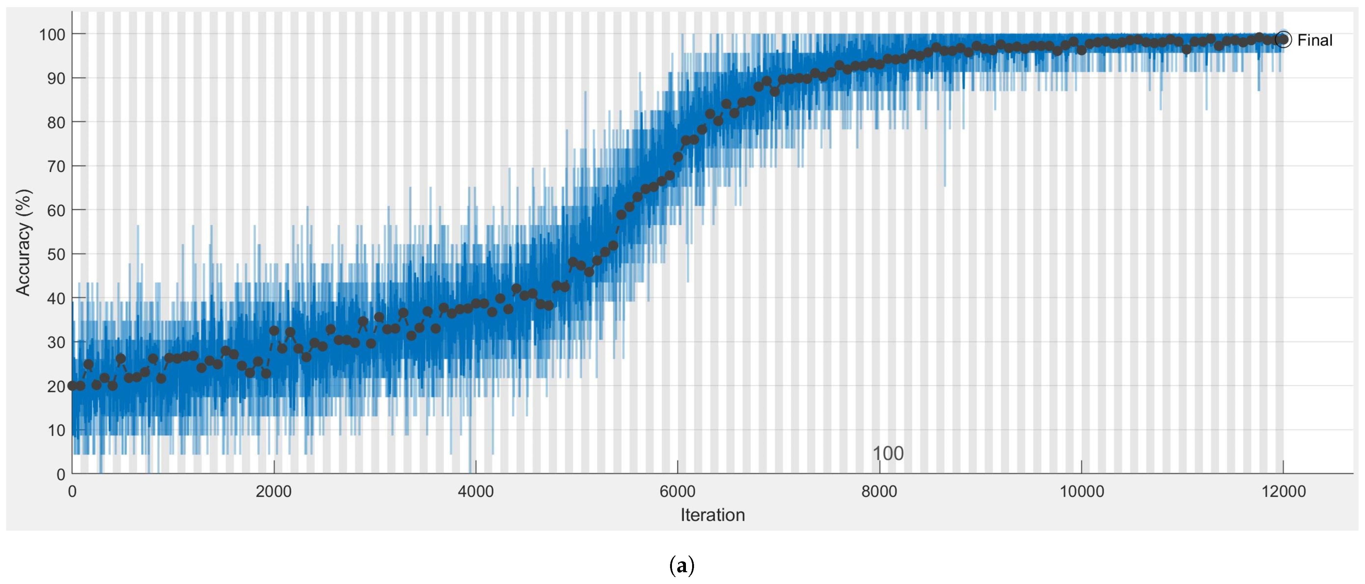
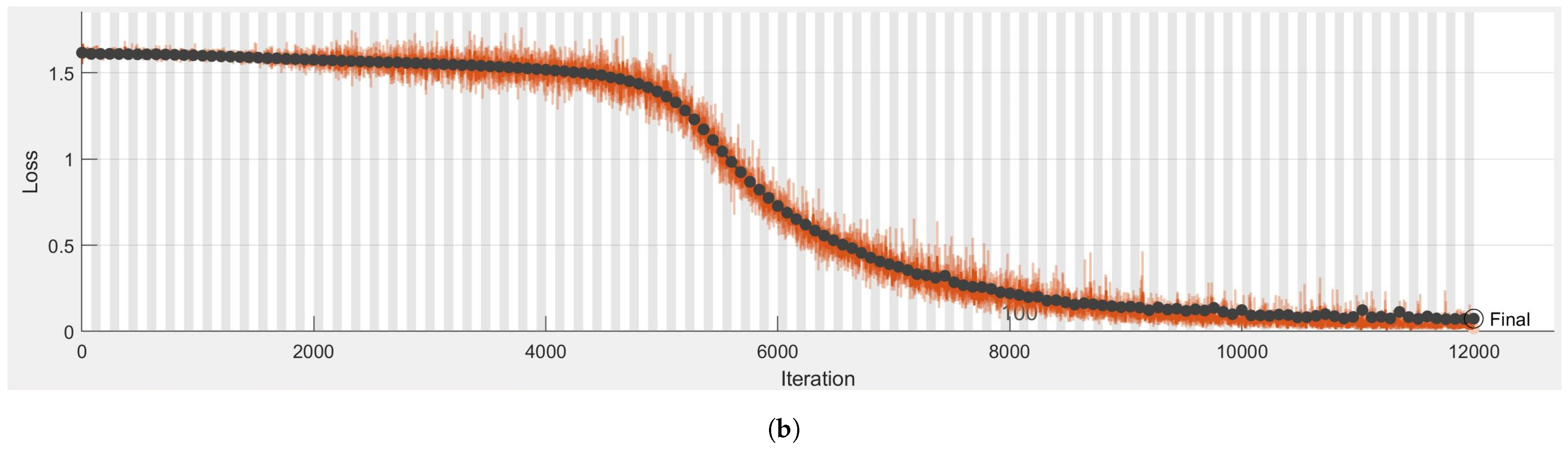
Figure 5a shows the network training process. As you can see, the learning process in the first 60 epochs was very slow, but in the further part, the accuracy gradually increased until it reached the level of 98.54% of correct results. One could observe a simultaneous adequate decrease in the level of loss in Figure 5b. No significant jumps in the line or reflection effect were observed in the learning process, which indicates that there was no over-fitting phenomenon. The learning process continued for 1218.7 s.
6. Results and Discussion
The studies were conducted classification into five categories. For the MuchSlower and Slower classes qualified those pairs images in which the object in the right image was farther from the lens than the object in the left image. This was to simulate the delay in sending the image from the right camera. The Regular class belonged to all those images in which the object in both images was the same distance from the camera. In contrast, the Faster and MuchFaster classes contain pairs of images in which the object in the right image was closer to the lens than the object in the left image. It was supposed to show the situation when the image from the left camera had a delay in sending relative to the image from the right camera. The distinction between the MuchSlower and Slower classes, as well as Faster and MuchFaster classes, was based on a larger or smaller difference in the distance between the object and the cameras. In order to determine these values, a hypothetical case of the observer moving at a speed of 30 km/h was assumed. This was to simulate the movement of a vehicle traveling at such a speed, on which there are two cameras. With the assumption of the error margin (measurement error) for correct synchronization in the distance from −22 mm to 22 mm, and knowing that the discrepancy of the distance of one frame at the image recording speed of 30 frames per second is 278 mm, the ranges of distance differences were calculated, which are presented in Table 1.
The process of training the network was carried out on the Train set and verified by data from the Validation set. The following results were obtained when classifying images from the Test set that did not participate in the training.
The analysis of the values obtained in the testing process of the proposed network model was carried out in the context of , , , and [26,27]. The relevant measures have been calculated in accordance with the following Formulas (1)–(4) and have been prepared for the obtained classification results.
where:
- –the sum of true positive results,
- –the sum of false-positive results,
- –the sum of true negative results,
- –the sum of false-negative results.
As a result of the training, five values of the coefficient of the probability of belonging a given pair of images to each of the possible classes were obtained. It is assumed that the highest of these values assigns a given sample to one of five classes. The greater the difference between the highest value and the other four values, the more convinced the model was of belonging. Therefore, it was important that the model not only assigned a given sample to the appropriate class but that the degree of its membership was as high as possible. Table 2 presents the average probability value for the predicted belonging to the appropriate class.
Summary of the results obtained for individual metrics is presented in Table 3. Each of them allows for the verification of the correctness of the network model learning process in a different respect.
Accuracy is one of the basic metrics that determine the percentage of correct answers in the entire set of obtained results. It is sensitive to differences in class size. The database used in this study has sets of individual classes of the same size, and the lowest accuracy is 98.86%, hence the conclusion that our research has high accuracy. The recall for all five categories was at least 95%, and in some cases even 100%. This indicates a very small number of false-negative matches (nine cases out of 615 cases studied). A high level of precision has been achieved, in each case, it is greater than 96%, which in turn says about the occurrence of a very small number of false-positive results (nine cases out of 615 cases studied). Specificity measures how well the model prevents false positives. The obtained minimum of 98% for each class is a very good achievement.
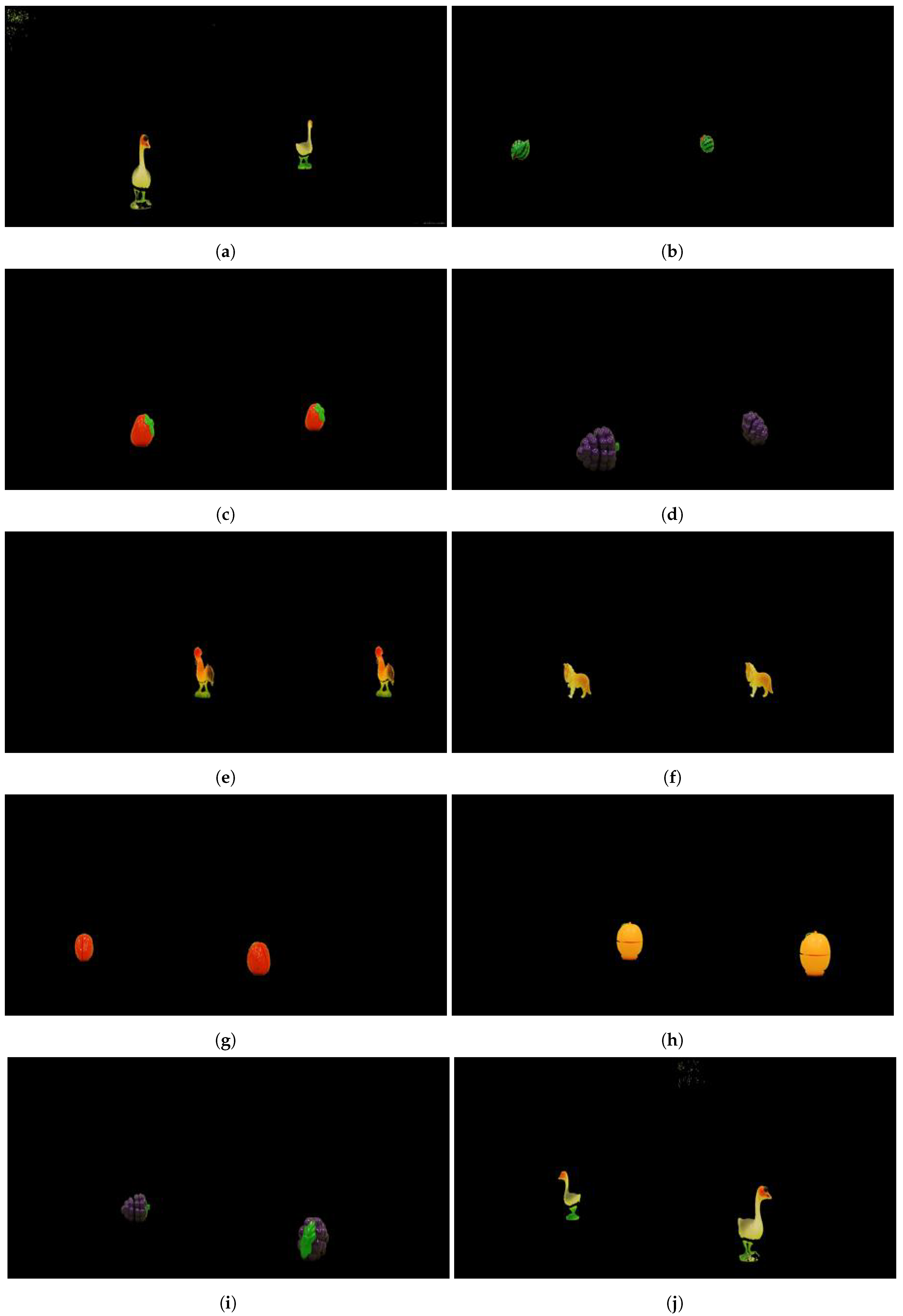
Overall, a very good classification result was obtained for the entire network model with a probability of 98.54%. Figure 6 shows the results obtained for the proposed network for sample image pairs from the Test set.
7. Conclusions
The work showed that it is possible to develop a tool in the form of CNN to detect synchronization errors in data transmission from two cameras. As shown, this process can be done using classification. The proposed method is a supplement for triggering systems for the simultaneous recording start of several cameras. As can be seen as a result of the conducted work, very good results were obtained as to the correct classification. A high percentage of the average probability in individual classes confirms the correctness of the results.
It is essential that the stereo pairs of images are acquired in a calibrated camera system, preferably canonical. Although it is not difficult to make such images, it is very difficult to find a ready-made database that meets such assumptions.
A certain limitation in the performance of the tests is also the equal distance between camera lenses during the acquisition of the stereo pair for all database samples. Therefore, it is allowed to use samples from different sources of the different distances between cameras, but only on the condition that the distance between the camera lenses is known, and its value is entered as an additional (necessary) parameter of the CNN model. This requires adapting the network architecture and re-learning it.
Maintaining parallelism in the position of the cameras is less important. For example, when one camera is slightly higher, or when the angle between the camera lenses is slightly less than 180 degrees, but only slight differences are allowed. Such a discrepancy does not affect the size of the object, which is the most important characteristic that determines the lack of synchronization being sought.
It is also very important that the stereo images of a given pair are recorded in a uniform manner and under uniform conditions. The easiest way to do this is to use identical image recording devices with identical settings. When entering data into the tensors, images are scaled, so individual samples may differ in size and resolution, but the components of a given sample must have the same size and resolution. It is in these assumptions that the information that the network learns is hidden. A big problem of the conducted research was the lack of access to the database containing stereo pairs of images in accordance with the assumptions mentioned above. Therefore, the study used its own database.
The photo database in which the location of the object of interest was located in different places of the photographed scene was used in the research, ensuring that the network does not learn the location but discrepancies in the size of the object. Therefore, the patterns recognized by the network are independent of offset. Logical analysis of the studied cases suggests that the parameter of the difference in the size of objects on the examined pair of images is a key parameter in determining whether there is a lack of synchronization between pairs of images. This feature determines the classification result, which at the same time leads to the conclusion that the model has a low tolerance for scaling images.
The presented work considers five cases, it is planned to expand the research by increasing the number of images, which will allow considering more cases (more classes). To this end, it is necessary to expand the author’s database. Work is already underway to change the way images are entered into the database in a more optimal way.
Noteworthy is the innovative way of entering two images into the CNN network with one input. Where the second image is, in a way, an extension of the first image with the next three components. It also turned out to be a good idea to perform some image preoperation by converting all pixels except the object of interest to black. This eliminated the unnecessary risk of the network learning the details of the environment instead of the object of interest.
The idea of using CNN to verify the synchronization of cameras in a stereo system is proven possible and returns very good results.
Author Contributions
Methodology and investigation and software and writing—original draft and visualization and formal analysis, J.K.; writing—review and editing, J.K. and M.K.; supervision and resources and funding acquisition, M.K. All authors have read and agreed to the published version of the manuscript.
Funding
This project was financed under the program of the Minister of Science and Higher Education under the name “Regional Initiative of Excellence” in the years 2019–2022 project number 020/RID/2018/19, and the amount of financing is 12,000,000 PLN.
Data Availability Statement
Not applicable.
Conflicts of Interest
The authors declare no conflict of interest.
References
- Roldán, J.J.; Peña-Tapia, E.; Garcia-Aunon, P.; Del Cerro, J.; Barrientos, A. Bringing adaptive and immersive interfaces to real-world multi-robot scenarios: Application to surveillance and intervention in infrastructures. IEEE Access 2019, 7, 86319–86335. [Google Scholar] [CrossRef]
- Musić, J.; Kružić, S.; Stančić, I.; Papić, V. Adaptive Fuzzy Mediation for Multimodal Control of Mobile Robots in Navigation-Based Tasks. Int. J. Comput. Intell. Syst. 2019, 12, 1197–1211. [Google Scholar] [CrossRef]
- Walter, M.R.; Antone, M.; Chuangsuwanich, E.; Correa, A.; Davis, R.; Fletcher, L.; Frazzoli, E.; Friedman, Y.; Glass, J.; How, J.P.; et al. A Situationally Aware Voice-commandable Robotic Forklift Working Alongside People in Unstructured Outdoor Environments. J. Field Robot. 2015, 32, 590–628. [Google Scholar] [CrossRef] [Green Version]
- Cadena, C.; Carlone, L.; Carrillo, H.; Latif, Y.; Scaramuzza, D.; Neira, J.; Reid, I.; Leonard, J.J. Past, present, and future of simultaneous localization and mapping: Toward the robust-perception age. IEEE Trans. Robot. 2016, 32, 1309–1332. [Google Scholar] [CrossRef] [Green Version]
- Beinschob, P.; Reinke, C. Graph SLAM based mapping for AGV localization in large-scale warehouses. In Proceedings of the 2015 IEEE International Conference on Intelligent Computer Communication and Processing (ICCP), Cluj-Napoca, Romania, 3–5 September 2015; IEEE: Hoboken, NJ, USA, 2015; pp. 245–248. [Google Scholar] [CrossRef]
- Huang, B.; Zhao, J.; Liu, J. A Survey of Simultaneous Localization and Mapping. arXiv 2019, arXiv:1909.05214. [Google Scholar]
- Chen, Y.; Wu, Y.; Xing, H. A complete solution for AGV SLAM integrated with navigation in modern warehouse environment. In Proceedings of the 2017 Chinese Automation Congress (CAC), Jinan, China, 20–22 October 2017; IEEE: Hoboken, NJ, USA, 2017; pp. 6418–6423. [Google Scholar] [CrossRef]
- Xue, B.; Cao, L.; Han, D.; Bai, X.; Zhou, F.; Jiang, Z. A DAISY descriptor based multi-view stereo method for large-scale scenes. J. Vis. Commun. Image Represent. 2016, 35, 15–24. [Google Scholar] [CrossRef]
- Zhang, S. High-speed 3-D shape measurement with structured light methods: A review. Opt. Lasers Eng. 2018, 106, 119–131. [Google Scholar] [CrossRef]
- Domínguez-Morales, M.; Domínguez-Morales, J.P.; Jiménez-Fernández, Á.; Linares-Barranco, A.; Jiménez-Moreno, G. Stereo Matching in Address-Event-Representation (AER) Bio-Inspired Binocular Systems in a Field-Programmable Gate Array (FPGA). Electronics 2019, 8, 410. [Google Scholar] [CrossRef] [Green Version]
- Wang, F.; Lü, E.; Wang, Y.; Qiu, G.; Lu, H. Efficient Stereo Visual Simultaneous Localization and Mapping for an Autonomous Unmanned Forklift in an Unstructured Warehouse. Appl. Sci. 2020, 10, 698. [Google Scholar] [CrossRef] [Green Version]
- Cruz-Santos, W.; Venegas-Andraca, S.E.; Lanzagorta, M. A QUBO Formulation of the Stereo Matching Problem for D-Wave Quantum Annealers. Entropy 2018, 20, 786. [Google Scholar] [CrossRef] [PubMed] [Green Version]
- Peng, J.; Xu, W.; Liang, B.; Wu, A.G. Pose Measurement and Motion Estimation of Space Non-cooperative Targets based on Laser Radar and Stereo-vision Fusion. IEEE Sens. J. 2018, 19, 3008–3019. [Google Scholar] [CrossRef]
- Peng, J.; Xu, X.; Liang, B.; Wu, A. Virtual Stereo-vision Measurement of Non-cooperative Space Targets for a Dual-arm Space Robot. IEEE Trans. Instrum. Meas. 2019, 69, 1–13. [Google Scholar] [CrossRef]
- Peng, J.; Xu, W.; Yuan, H. An Efficient Pose Measurement Method of a Space Non-Cooperative Target Based on Stereo Vision. IEEE Access 2017, 5, 22344–22362. [Google Scholar] [CrossRef]
- Kulawik, J. The effect of edge operation on the detection of the reference element using the FREAK and SURF methods. In Monografia Naukowa “Mała Wielka Nauka”; Solarczyk, P., Ed.; Wydawnictwo Fundacji Promovendi: Łódź, Poland, 2017; Volume 1, pp. 26–41. [Google Scholar]
- Domínguez-Morales, M.J.; Jiménez-Fernández, Á.; Jiménez-Moreno, G.; Conde, C.; Cabello, E.; Linares-Barranco, A. Bio-Inspired Stereo Vision Calibration for Dynamic Vision Sensors. IEEE Access 2019, 7, 138415–138425. [Google Scholar] [CrossRef]
- Hartley, R.; Zisserman, A. Multiple View Geometry in Computer Vision; Cambridge University Press: Cambridge, UK, 2003. [Google Scholar]
- Choraś, M.; Giełczyk, A.; Demestichas, K.P.; Puchalski, D.; Kozik, R. Pattern Recognition Solutions for Fake News Detection. In Computer Information Systems and Industrial Management; Saeed, K., Homenda, W., Eds.; Springer: Berlin/Heidelberg, Germany, 2018; Volume 11127, pp. 130–139. [Google Scholar]
- Ksieniewicz, P.; Choraś, M.; Kozik, R.; Woźniak, M. Machine Learning Methods for Fake News Classification. In Intelligent Data Engineering and Automated Learning–IDEAL 2019; Lecture Notes in Computer Science; Yin, H., Camacho, D., Tino, P., Tallón-Ballesteros, A., Menezes, R., Allmendinger, R., Eds.; Springer: Berlin/Heidelberg, Germany, 2019; Volume 11872, pp. 332–339. [Google Scholar]
- Woźniak, M.; Połap, D. Adaptive neuro-heuristic hybrid model for fruit peel defects detection. Neural Netw. 2018, 98, 16–33. [Google Scholar] [CrossRef] [PubMed]
- Ke, Q.; Zhang, J.; Wei, W.; Połap, D.; Woźniak, M.; Kośmider, L.; Damaševĭcius, R. A neuro-heuristic approach for recognition of lung diseases from X-ray images. Expert Syst. Appl. 2019, 126, 218–232. [Google Scholar] [CrossRef]
- Woźniak, M.; Połap, D. Bio-inspired methods modeled for respiratory disease detection from medical images. Swarm Evol. Comput. 2018, 41, 69–96. [Google Scholar] [CrossRef]
- Kubanek, M. A New Approach to Speech Recognition Using Convolutional Neural Networks. In Mathematical Modeling in Physics and Engineering (MMPE); Wydawnictwo Wydziału Zarządzania Politechniki Częstochowskiej: Czestochowa, Poland, 2018; pp. 24–30. [Google Scholar]
- Kubanek, M.; Bobulski, J.; Kulawik, J. A Method of Speech Coding for Speech Recognition Using a Convolutional Neural Network. Symmetry 2019, 11, 1185. [Google Scholar] [CrossRef] [Green Version]
- Goodfellow, I.; Bengio, Y.; Courville, A. Deep Learning. Systemy Uczące Się; Wydawnictwo Naukowe PWN: Warsaw, Poland, 2018. [Google Scholar]
- Patterson, J.; Gibson, A. Deep Learning. Praktyczne Wprowadzenie; Wydawnictwo Helion: Gliwice, Poland, 2018. [Google Scholar]
- Chollet, F. Deep Learning. Praca z Językiem Python i Biblioteką Keras; Wydawnictwo Helion: Gliwice, Poland, 2019. [Google Scholar]
- Géron, A. Uczenie Maszynowe z Użyciem Scikit-Learn i TensorFlow. Wydanie II; Wydawnictwo Helion: Gliwice, Poland, 2020. [Google Scholar]
- © 1994–2020 The MathWorks, Inc. MATLAB Documentation; The MathWorks, Inc.: Natick, MA, USA, 2020; Available online: https://uk.mathworks.com/help/matlab/index.html (accessed on 1 December 2020).
Figure 1.
An example of a pair of images. (a) The image from the left camera. (b) The image from the right camera.
Figure 1.
An example of a pair of images. (a) The image from the left camera. (b) The image from the right camera.

Figure 2.
A set of photographed objects.

Figure 3.
Examples of image pairs for all five cases for the “orange” and “strawberry” objects. (a) MuchSlower. (b) Slower. (c) Regular. (d) Faster. (e) MuchFaster.
Figure 3.
Examples of image pairs for all five cases for the “orange” and “strawberry” objects. (a) MuchSlower. (b) Slower. (c) Regular. (d) Faster. (e) MuchFaster.


Figure 4.
Convolutional Neural Network structure.

Figure 5.
The characteristics for the training progress and loss for Convolutional Neural Network (CNN). (a) The characteristics for the training progress. (b) The characteristics for the training loss.
Figure 5.
The characteristics for the training progress and loss for Convolutional Neural Network (CNN). (a) The characteristics for the training progress. (b) The characteristics for the training loss.


Figure 6.
Sample results of the proposed network for pairs of images from the Test set. (a) MuchSlower 100.00%. (b) MuchSlower 99.90%. (c) Slower 100.00%. (d) Slower 99.90%. (e) Regular 99.20%. (f) Regular 100.00%. (g) Faster 99.80%. (h) Faster 99.90%. (i) MuchFaster 98.50%. (j) MuchFaster 99.20%.
Figure 6.
Sample results of the proposed network for pairs of images from the Test set. (a) MuchSlower 100.00%. (b) MuchSlower 99.90%. (c) Slower 100.00%. (d) Slower 99.90%. (e) Regular 99.20%. (f) Regular 100.00%. (g) Faster 99.80%. (h) Faster 99.90%. (i) MuchFaster 98.50%. (j) MuchFaster 99.20%.


Table 1.
The range of differences in object distance in the right image compared to the left image.
| Event | Threshold [mm] |
|---|---|
| Much Slower | from −578 to −301 |
| Slower | from −300 to −23 |
| Regular | from −22 to 22 |
| Faster | from 23 to 300 |
| Much Faster | from 301 to 578 |
Table 2.
The average probability value for the predicted belonging to the appropriate class.
| Event | Average Probability [%] |
|---|---|
| MuchSlower | 97.76 |
| Slower | 97.70 |
| Regular | 98.17 |
| Faster | 95.61 |
| MuchFaster | 97.99 |
Table 3.
Appropriate metrics calculated for the obtained results of testing the correctness of the operation of the proposed network.
Table 3.
Appropriate metrics calculated for the obtained results of testing the correctness of the operation of the proposed network.
| Event | Accuracy | Recall | Specificity | Precision |
|---|---|---|---|---|
| (A) [%] | (R) [%] | (S) [%] | (P) [%] | |
| MuchSlower | 99.67 | 98.37 | 100.00 | 100.00 |
| Slower | 99.67 | 100.00 | 99.59 | 98.40 |
| Regular | 99.67 | 98.37 | 100.00 | 100.00 |
| Faster | 98.86 | 95.93 | 99.59 | 98.33 |
| MuchFaster | 99.19 | 100.00 | 98.98 | 96.09 |
Publisher’s Note: MDPI stays neutral with regard to jurisdictional claims in published maps and institutional affiliations. |
© 2021 by the authors. Licensee MDPI, Basel, Switzerland. This article is an open access article distributed under the terms and conditions of the Creative Commons Attribution (CC BY) license (http://creativecommons.org/licenses/by/4.0/).
Share and Cite
MDPI and ACS Style
Kulawik, J.; Kubanek, M. Detection of False Synchronization of Stereo Image Transmission Using a Convolutional Neural Network. Symmetry 2021, 13, 78. https://doi.org/10.3390/sym13010078
AMA Style
Kulawik J, Kubanek M. Detection of False Synchronization of Stereo Image Transmission Using a Convolutional Neural Network. Symmetry. 2021; 13(1):78. https://doi.org/10.3390/sym13010078
Chicago/Turabian StyleKulawik, Joanna, and Mariusz Kubanek. 2021. "Detection of False Synchronization of Stereo Image Transmission Using a Convolutional Neural Network" Symmetry 13, no. 1: 78. https://doi.org/10.3390/sym13010078
Note that from the first issue of 2016, this journal uses article numbers instead of page numbers. See further details here.