Inhibition and Hydrodynamic Analysis of Twin Side-Hulls on the Porpoising Instability of Planing Boats


National Key Laboratory of Science and Technology on Autonomous Underwater Vehicle, Harbin Engineering University, Harbin 150001, China
*
Author to whom correspondence should be addressed.
J. Mar. Sci. Eng. 2021, 9(1), 50; https://doi.org/10.3390/jmse9010050
Submission received: 2 December 2020
/
Revised: 30 December 2020
/
Accepted: 31 December 2020
/
Published: 5 January 2021
(This article belongs to the Special Issue CFD Simulations of Marine Hydrodynamics)
Abstract
:A comparative analysis of the hydrodynamic performance of a planing craft in the monomer-form state (MFS) and trimaran-form state (TFS) was performed, and the inhibition mechanism of twin side-hulls on porpoising instability was evaluated based on the numerical method. A series of drag tests were conducted on the monomer-form models with different longitudinal locations of the center of gravity (Lcg); the occurrence of porpoising and the influence of Lcg on porpoising by the model was discussed. Then, based on the Reynolds-averaged Navier–Stokes (RANS) solver and overset grid technology, numerical simulations of the model were performed, and using test data, the results were verified by incorporating the whisker spray equation of Savitsky. To determine how the porpoising is inhibited in the TFS, simulations for the craft in the MFS and TFS when porpoising were performed and the influence of side-hulls on sailing attitudes and hydrodynamic performance at different speeds were analyzed. Using the full factor design spatial sampling method, the influence of longitudinal and vertical side-hull placements on porpoising inhibition were deliberated, and the optimal side-hull location range is reported and verified on the scale of a real ship. The results indicate that the longitudinal side-hull location should be set in the ratio (a/Lm) range from 0.1 to 0.3, and vertically, the draft ratio (Dd/Tm) should be less than 0.442. Following these recommendations, porpoising instability can be inhibited, and lesser resistance can be achieved.
1. Introduction
Stability problems associated with high-speed planing crafts have long been a notable research focus for designers, even in calm waters. It is well known that due to the existence of longitudinal or transverse instability, many kinds of dangerous accidents may occur [1]. The abrupt variation of trim causes the self-induced heave and pitch oscillations, which has been named porpoising [2]. In severe cases, the bow even suffers a violent attack and generates greater resistance in fast vessels, which threatens the safety of on-board personnel and equipment. The transverse instability causes the sudden emergence of large heeling, leads to a loss of course-keeping ability, and facilitates chine walking [3].
Considering the reasons outlined above and the associated adverse situations, it is important for engineers to control the longitudinal and transverse instability of high-speed crafts. In terms of the longitudinal instability, since the porpoising was observed during the test conducted by Clement and Blount [4], Blount and Codega [5] analyzed the dynamic instability problem, focusing on the nonlinear vibration of the planing craft through the test method, and the suggested criterion conditions for the unstable motion were given. Katayama and Yoshiho [6] conducted a series of performance tests on planing crafts, concretely involving accelerated longitudinal motion and porpoising instability, which provides crucial comparative data for many scholars. In recent years, porpoising theory has been applied in some studies based on established numerical methods [7] and Savitsky’s work [8,9]; those studies were primarily concerned with the inhibition of trim instability by appendages such as interceptors, trim tabs, and wedges [10,11,12]. The interceptor is a thin vertical plate protruding from the stern that is installed at the bottom edge. Mehran et al. [13] ascertained that the inhibition mechanism of the interceptor on porpoising in the planing boat, and Mansoori et al. [14,15] further analyzed the influence of boundary layer thickness, interceptor height, and span on the inhibition of porpoising and navigation resistance, and demonstrated that the combination of trim tab and interceptor with the same size is more beneficial to control the trim and reduce the resistance than the single interceptor. In addition, to develop a craft design utilizing an interceptor that included six heights at distinct positions of the stern bottom, Ahmet and Baris [16] tested resistance and sailing attitudes and reported that for the same-size interceptor, the effect of drag reduction and porpoising inhibition was gradually reduced when installed at the interval from keel to bilge line. Hongjie et al. [17] and Hanbing et al. [18] calculated the porpoising of a planing boat in a uniform incoming flow, indicating that moving forward of the center of gravity could reduce the resistance peak value, which is beneficial to avoid porpoising.
Regarding transverse instability research, owing to the interference of many nonlinear factors and high calculation costs, most studies merely involved model test and improving the calculation method, as discussed in Refs. [19,20,21,22,23,24,25]. This research is not involved in the transverse stability of the planing boat because the installing of twin side-hulls widens the transverse weight distribution of the vessel, the transverse righting moment increases, which makes the transverse stability of the craft better than that of the monomer-form.
However, well-known porpoising instability restrains the maximum speed of high-speed planing crafts, but it can be controlled by using external devices, such as trim tabs, interceptors, side-hulls, etc. The doctoral thesis of Yi [26] indicated that a high-speed trimaran planing craft was beneficial to improve longitudinal stability, but it increased the resistance at lower speeds. So a conceptual planing boat, capable of freely retracting and releasing the twin side-hulls, is proposed in this research. At lower speeds, it maintains the monomer-form state (MFS), and at higher speeds, it expands into the trimaran-form state (TFS) to inhibit the porpoising and improve the longitudinal stability. But due to the strong interference of nonlinear factors and the high test cost, there are no or few studies analyzing the inhibition of twin side-hulls on porpoising.
Therefore, the hydrodynamic performance of twin side-hulls and their inhibiting effect on the porpoising instability in high-speed planning crafts were analyzed in this research. And a series of tests were conducted on the monomer-form models with different longitudinal locations of the gravity center (Lcg), and the influence of the Lcg on porpoising was determined. Then, based on the comparisons of the numerical (CFD) setup, simulations of the test model were performed, and the calculated results were verified using the whisker spray equation of Savitsky [27]. Further, the inhibition mechanism of the side-hulls on porpoising was ascertained, and a comparative analysis of the hydrodynamics of the planing craft in the MFS and TFS was performed. Finally, the influence of longitudinal and vertical side-hull locations on inhibiting porpoising was determined, and the optimal location range is provided.
2. Experimental Setup
2.1. Model Design
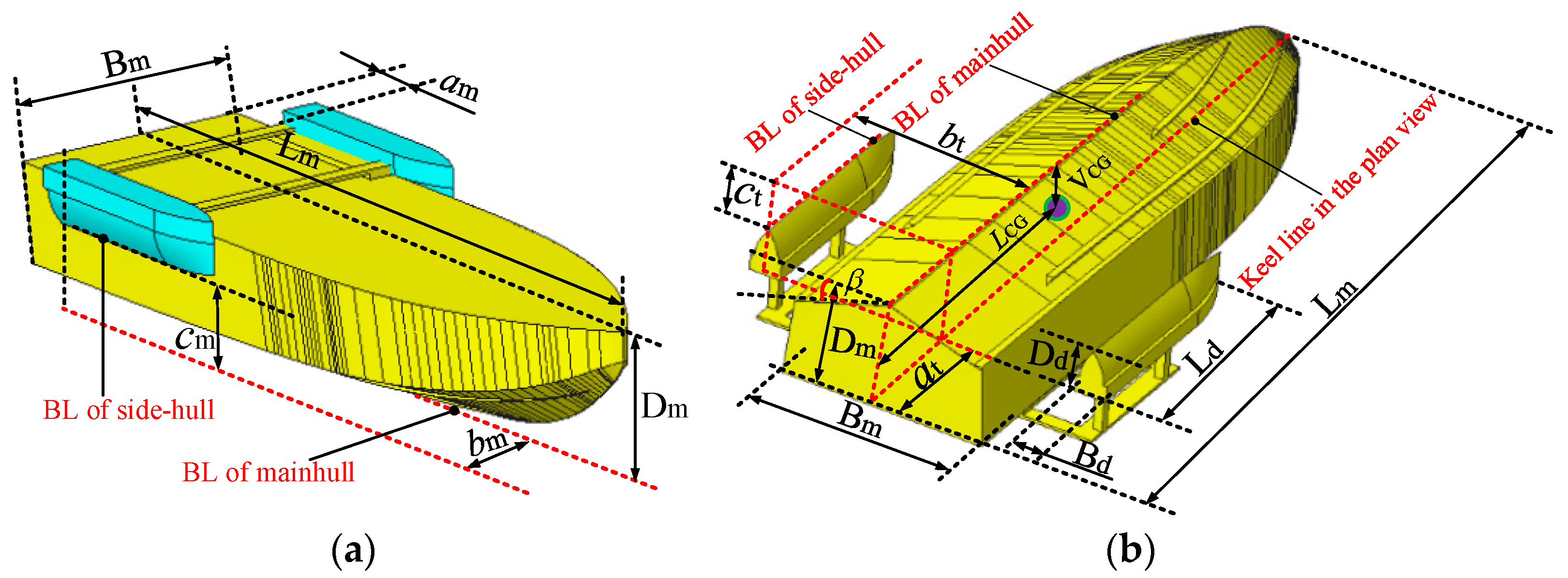
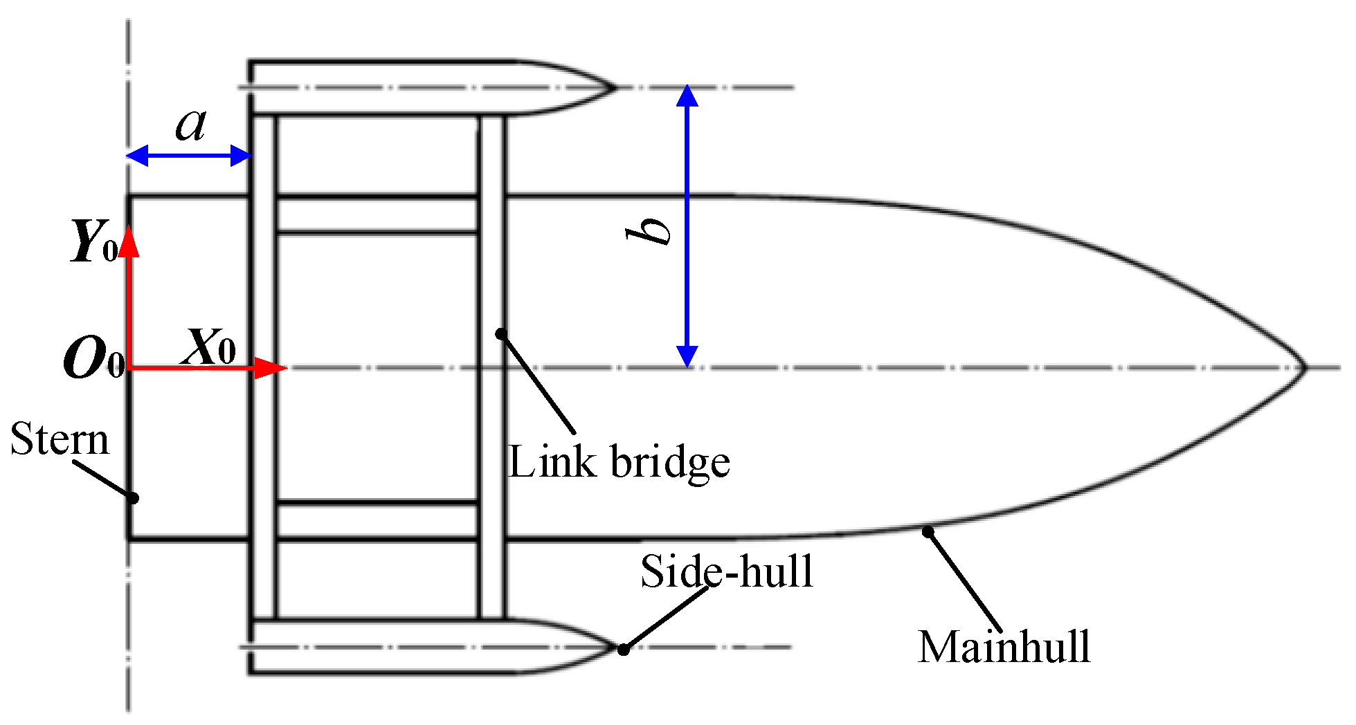
This study took a 1:2.5-scale test model of an actual planing hull with twin position-adjustable side-hulls as a research object. The twin side-hulls can be synchronously placed in any longitudinal, horizontal, and vertical positions of the ship broadsides within a certain scale range by the variable-structure link bridge. When on a relatively stable seas, the craft will pack up the twin side-hulls and sail forward quickly in the monomer-form state (MFS), as shown in Figure 1a. When encountering high sea conditions, it will put down the twin side-hulls and sail stably in the TFS, as shown in Figure 1b. Main geometric details of the planing hull in different navigation states are listed in Table 1.
The hard chine test model (main hull), built-in wood, was square-tailed and non-stepped, had a larger knuckle line width, a plurality of spray deflectors with variant dimensions were symmetrically installed at the main hull bottom to improve its seakeeping and reduce resistance in calm water. The twin side-hulls were arranged at both broadsides of the main hull by a link bridge, were thin and sharp in cross-section, slender in whole and vertical in the bilge, provide bare buoyancy and hydrodynamic lift but improved directional stability. The molded lines of the main hull and side-hulls are presented in Figure 2. For convenient adjustment to the center of gravity (CG) position in the TFS and making the model easier to slide, the twin side-hulls were initially designed on both sides of the rear of the main hull as shown in Figure 1b, and the specific location is listed in Table 1.
2.2. Model Test
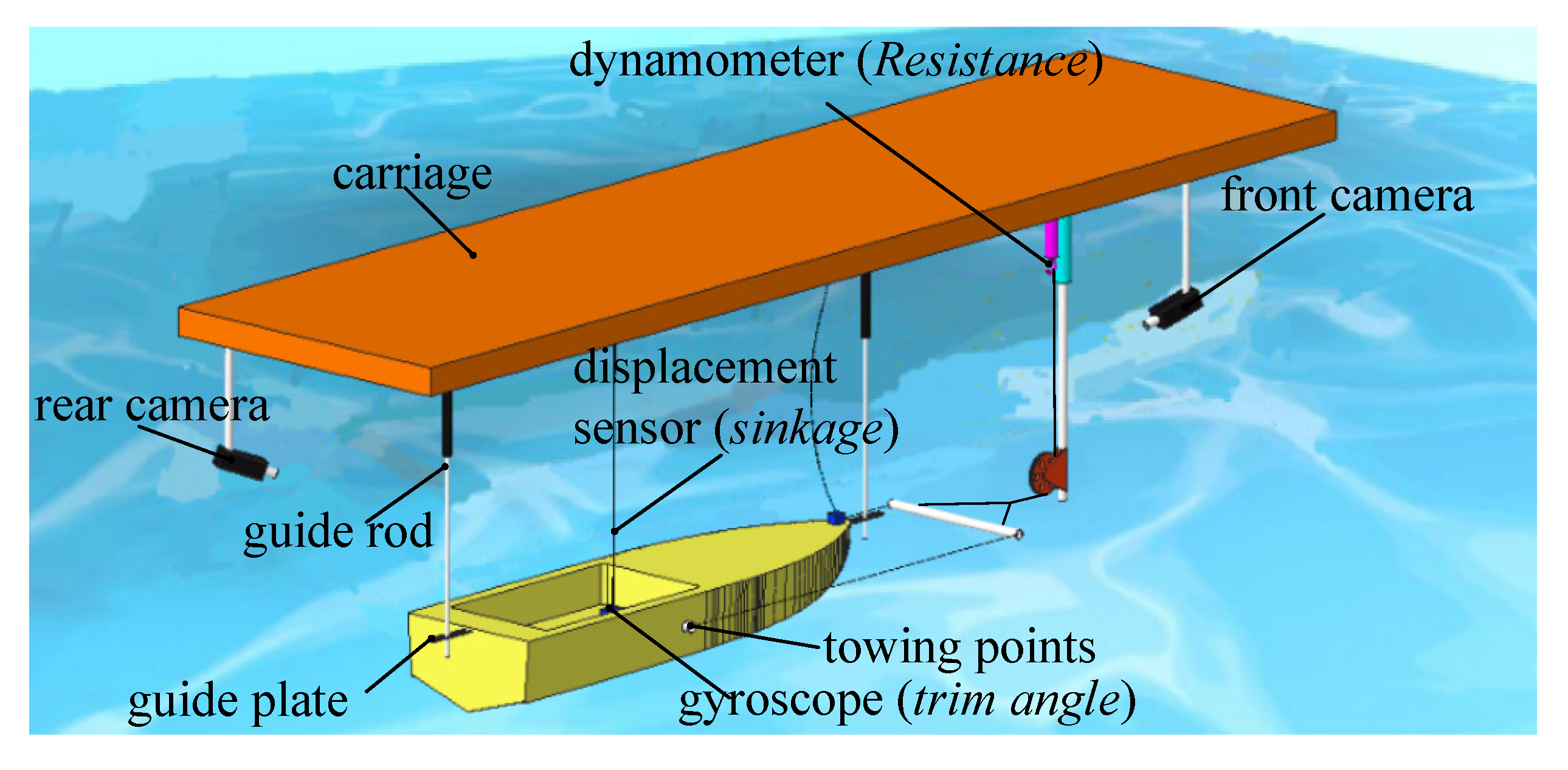
All model tests were conducted in the towing tank (510 m × 6.5 m × 6.8 m) of the High-speed Hydrodynamic Laboratory of Special Aircraft Research Institute of China. Owing to the higher test cost, only the towing tests of the model in the MFS were completed, and considering that the twin side-hulls were far higher than the waterline when packed up in the MFS, both were not installed in the test process, the schematic diagram of the experimental setup is presented in Figure 3.
The model was attached to a carriage (0.1%), and two guide robs were also fixed in the carriage, separately inserted into the guide plates of the bow and stern to prevent yaw and roll motion; the towing points were located at the broadside and aligned with the center of gravity (CG). The cable-extension displacement sensor (0.01 mm) and the gyroscope (0.01°) were fixed at the CG to measure the sinkage and dynamic trim, the electronic dynamometer (0.02 kg) was mounted on the carriage, pulled the tow bar for measuring the resistance, and the accuracy of the above measuring instruments is presented in the corresponding brackets. Moreover, the front and rear cameras were fixed on the forward and aft of the carriage to capture the flow phenomena of the model sailing in calm water.
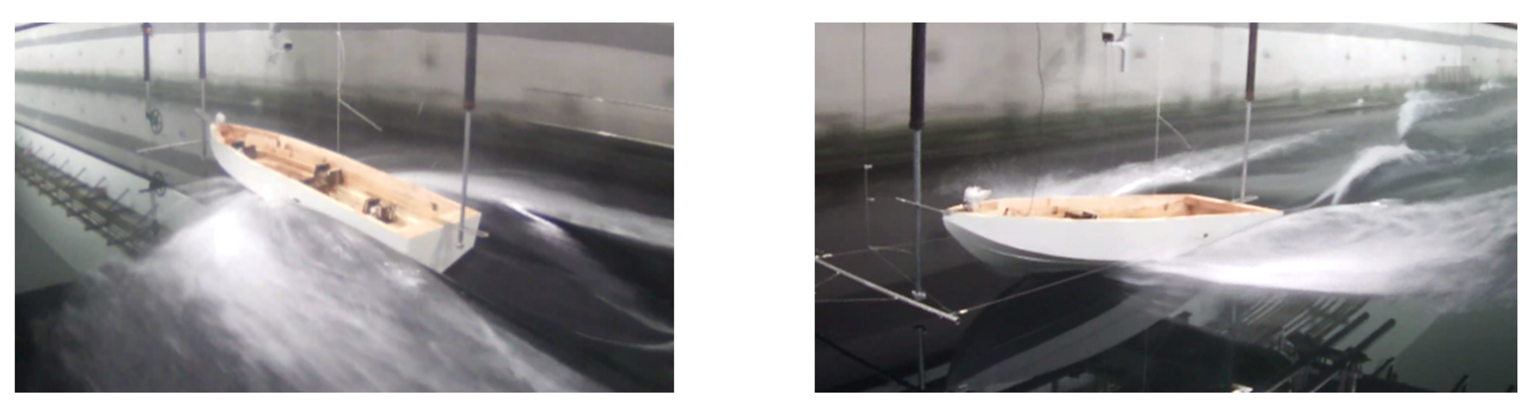
In the model tests, aimed at the two displacements and three longitudinal positions of the CG, four conditions were designed, as shown in Table 2. The towed speeds of the model were 3–13 m/s (length Froude numbers Fr = 0.63–2.72) or until porpoising occurred. The wave surface condition around the model and the stern wake in the distance were clearly captured, as presented in Figure 4, which shows the photographs from various perspectives of the model at Fr = 1.26 under condition two, and subsequently, a Longitudinal location of CG/Main hull length (Lcg/Lm) ratio of 0.38 occurred under condition two.
2.3. Experimental Results
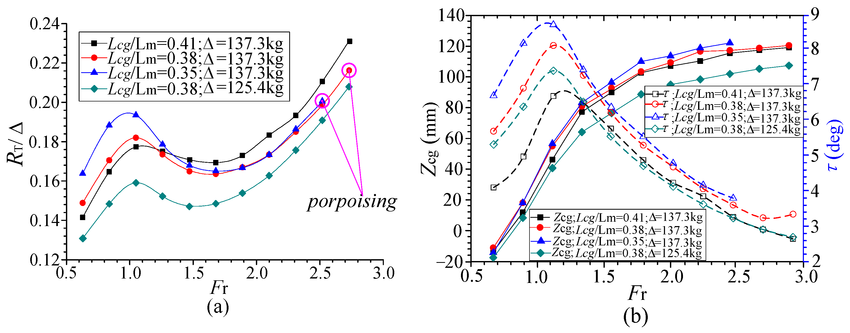
The measured parameters mainly include total resistance RT, sinkage Zcg, and trim angle τ when sailing stably; the RT was treated into the dimensionless form of RT/∆. The test results on the RT, Zcg, and τ of the monomer-form model under different conditions are shown in Figure 5.
Combing test phenomena and results, we found that at low speeds (Fr < 1.05), the bow was gradually lifted upwards as the speed increased. At the semi-planing state (Fr = 1.05), the sinkage and trim angle increased significantly. When crossing the resistance peak, entering the planing regime (Fr > 1.05), the RT appeared to be notably reduced; however, after descending to a certain threshold, the RT rose and exceeded the previous peak as the speed further increased. When Fr > 2.31, the Zcg increased slowly, but the τ always reduced as the speed increased during the planing stage.
For the model with equal displacement during the semi-planing state, as the Lcg moved backward, the resistance peak increased. When Fr > 1.05, as speed further increased, the more the Lcg moves backward within a certain scale, the more the RT decreased, but the Zcg and τ increased. In addition, when the Lcg remained at the same and speed increased, the RT, Zcg, and τ of the small-displacement boat were all less than those of the large-displacement boat, especially for the small-displacement boat, RT is lesser when crossing the resistance peak.
The porpoising of the model under conditions two and three occurred at Fr = 2.73 (v = 13 m/s) and 2.52 (v = 12 m/s), respectively. From the videos recorded in the experiment, we observed that the coupled heave and pitch oscillation amplitudes under condition three were extremely larger compared with condition two, which shows that when Lcg becomes increasingly backward, porpoising occurs more easily, and the oscillation amplitudes are even larger it limits the maximum speed.
3. CFD Setup
3.1. The Numerical Method
To simulate the viscous flow field around the sailing vessel, the governing equations of viscous incompressible fluid were introduced, and that were solved based on the Finite Volume Method (FVM) described in Ref. [28]; the main CFD solver is the platform of Star-CCM+, the Reynolds-averaged Navier–Stokes (RANS) and continuity equations jointly constitute the governing equations, and as follows
where ui and uj are the time mean of the velocity component, (i, j = 1, 2, 3), p is the pressure mean, ρ is the fluid density, μ is the coefficient of dynamic viscosity, is the Reynolds stress term, Si represents the generalized source term.
To close the governing equations, the Shear Stress Transport turbulence (SST) k–ω model [29] was adopted to calculate the Reynolds stress term in this research. Despite the existence of the strong adverse pressure gradient, the RANS model has been shown to be inaccurate and has some limitations as discussed in Refs. [30,31,32], but the SST k–ω turbulence model is still widely used to deal with high Reynolds number flow problems and has higher precision on solving the flow field around the high-speed planing craft [33].
Moreover, the volume of fluid (VOF) method, proposed by Nichols and Hirt [34,35] in 1981, was also used to track the change of the free surface in this research. In the VOF method, the most critical aspect is obtaining the volume ratio function (F) of the specified fluid occupancy in a grid cell. When the calculation of the F values in each grid cell is completed, the motion interface of the liquid-gas, two-phase flow can be tracked.
Then, to acquire the hull position, based on velocity and pressure in the flow field, the centroid motion theorem and centroid moment of motion theorem were used as follows
where is the momentum of the model, (p, q, r) is the angular velocity, (X, Y, Z) is the combined force, is the momentum moment relative to the CG, (u, v, w) is the speed and (L, M, N) is the combined moment.
and can be solved as below
where , and are the shear stress, pressure, and gravity, respectively. S is the hull surfaces. is the displacement of mesh nodes, and is the displacement of CG.
The overset-grid method, as described in Ref. [36], was adopted due to the complex hull motion. The solver procedure of the numerical method is shown in Figure 6. When variations of the forces and moments were less than the tolerance (ε) or the total iteration time (T) reaches, the calculation was terminated.
In the post-processing, the pressure, shear force, unit node coordinates at each unit are known; thus, the longitudinal moment of the side-hulls to CG can be calculated by integrating the element moments to the CG, and the dimensionless form as follows
where and are the local normal vector of the grid element and the displacement relative to the CG, respectively, Sd represents the surface area of twin side-hulls.
Likewise, adopting the same integral strategy, the dimensionless forms of the resistance and lift for the twin side-hulls are acquired as follows:
3.2. Computational Domains and Boundary Conditions
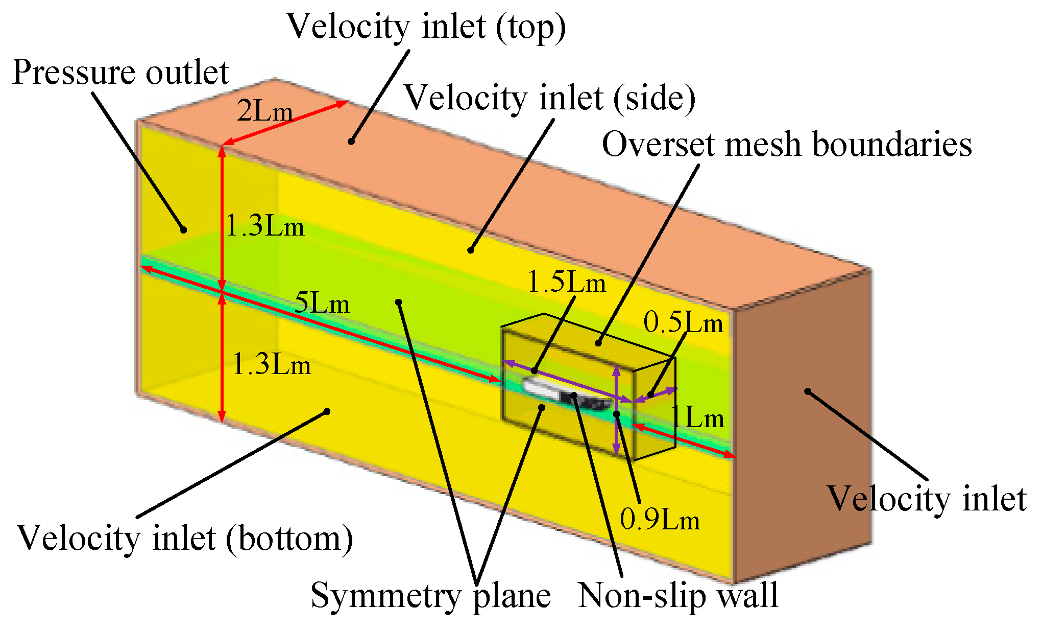
To prevent the reflection of waves in the computational domain and obtain a better precision, the domain should be no less than five times the hull length (Lm) [37]; thus, it was designed to a cuboid region with dimensions of 7.5 Lm × 2 Lm × 2.6 Lm, and its specific dimensions and the boundary conditions were depicted in Figure 7. Considering the symmetry of the model and flow field, only half a domain of the model was established to reduce the simulation duration.
To obtain a better simulation on the sailing attitudes of model, the overset region was embedded in the background region; the boundary conditions were set as follows: The background region, incoming-flow inlet, top, bottom, and side were all set to the velocity inlet, the outlet was the pressure outlet, and the middle longitudinal section was a symmetry plane; for the overset region, the mid-ship section was still a symmetry plane, the ambient planes were set to the overset mesh boundaries, and the hull body was defined as the non-slip wall.
3.3. Mesh Generation
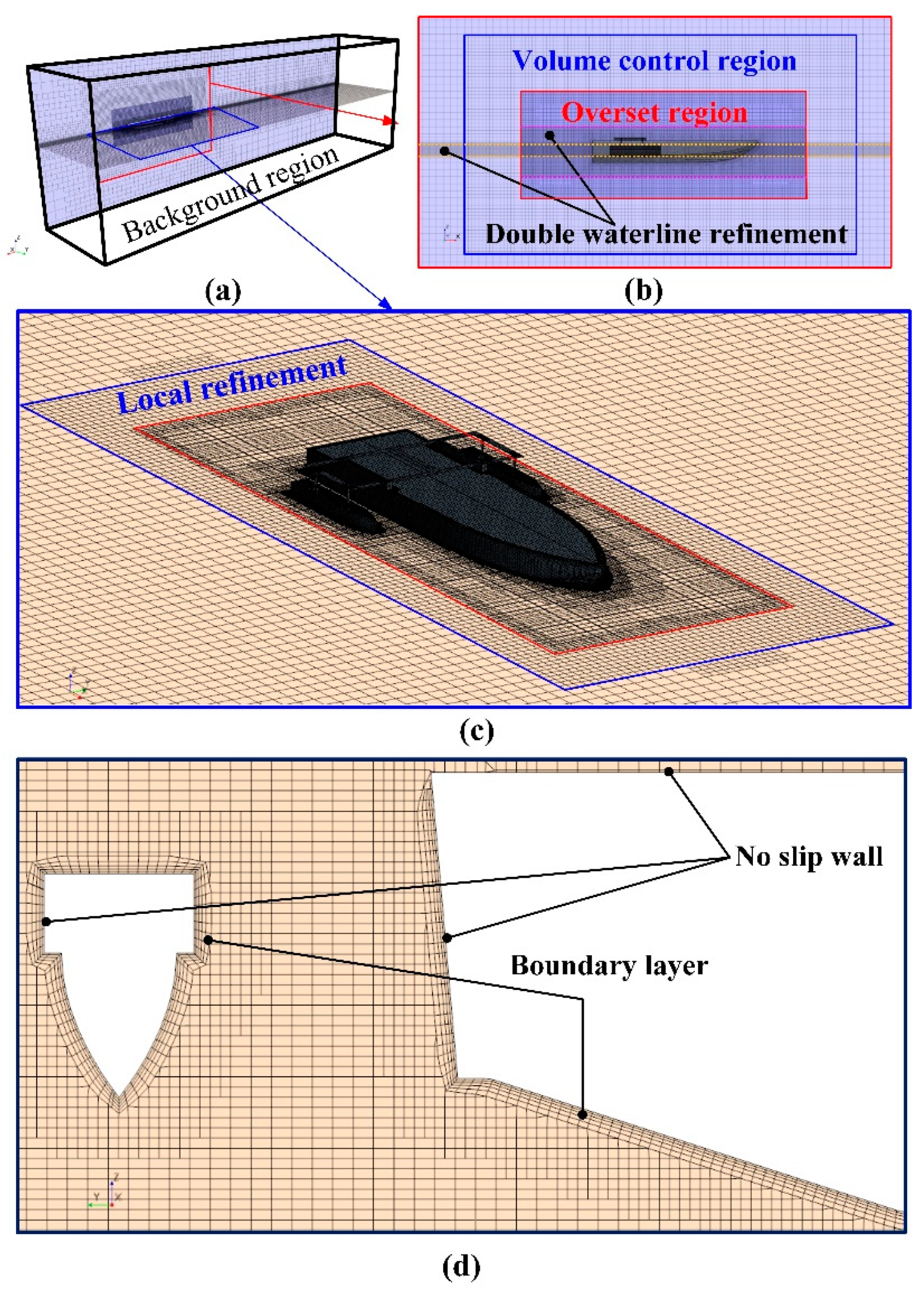
The grids in the background and overset region were automatically generated, as shown in Figure 8, and the grids of the two regions defined as follows: The cutting hexahedron grids were mainly used to discretize the background region, both the cutting hexahedron grids and the prismatic layer grids were selected to fill the overset region due to the complex geometrical details of the hull body. To obtain the more accurate flow field around the hull, the circumambience of the hull was refined by the smaller hexahedron grids in the volume control region; for the grids around the free surfaces in the two regions, that were set to more than twenty layers in the vertical direction to clearly capture the change of free surface; and the boundary layer grids were imposed on the surface of hull body.
3.4. Wall Non-Dimensional Distance of the First Layer Grid (y+) and Time Step Set-Up
To obtain the accurate stress and pressure of the flow field around the hull, wall functions, and boundary layer grids were required, referred to the Ref. [37]. The y+ value was ascertained as below
where y+ and y separately represent the non-dimensional distance and the height of the first layer grid, U is the speed of vessel, L is the waterline length of the vessel, υ is the fluid viscosity coefficient and Re represents the Reynolds number.
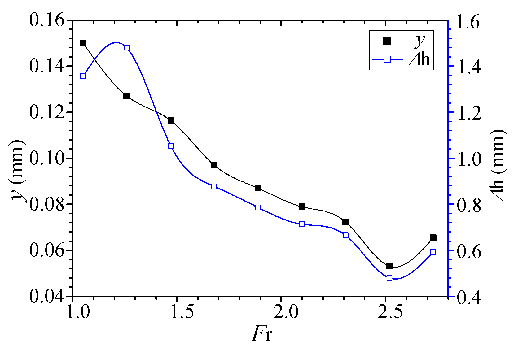
In this research, five boundary layers were adopted with a grid growth rate of 1.3. The generated boundary layer grids on the hull body are presented in Figure 8d. The details of when the y+ = 250, the y values, and total boundary layer grid reached thicknesses ∆h at different speeds are shown in Figure 9.
In addition, considering the time step of iteration (∆t) depends on flow characteristics in the implicit unsteady simulation, as discussed in Ref. [38], the range of ∆t is initially defined as follows:
The maximum number of internal iterations and total calculation time were set to five times and 15 s, respectively.
4. Numerical Simulation Verification
4.1. Grid Parameters
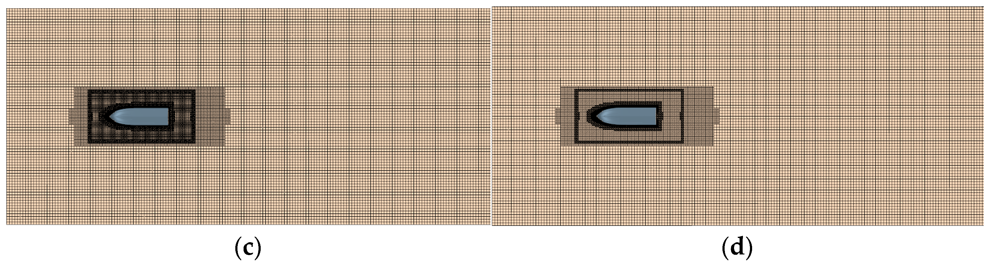
To verify the convergence of the grid, four grids were designed, whose sizes on the hull surface and in the background region were the same, but the grid sizes in the overset region, volume control region, and around the free surface increased with the refinement ratio (, Lg = 1 m), the grid parameters of four grids are shown in Table 3, and the grids around the hull and the free surface are presented in Figure 10. Then, the sailing of the model in calm water was simulated, and the results of resistance were compared with the test. The numerical setting is consistent with the Section 3, and the towing speed Fr = 1.26 (v = 6 m/s) was selected for verification.
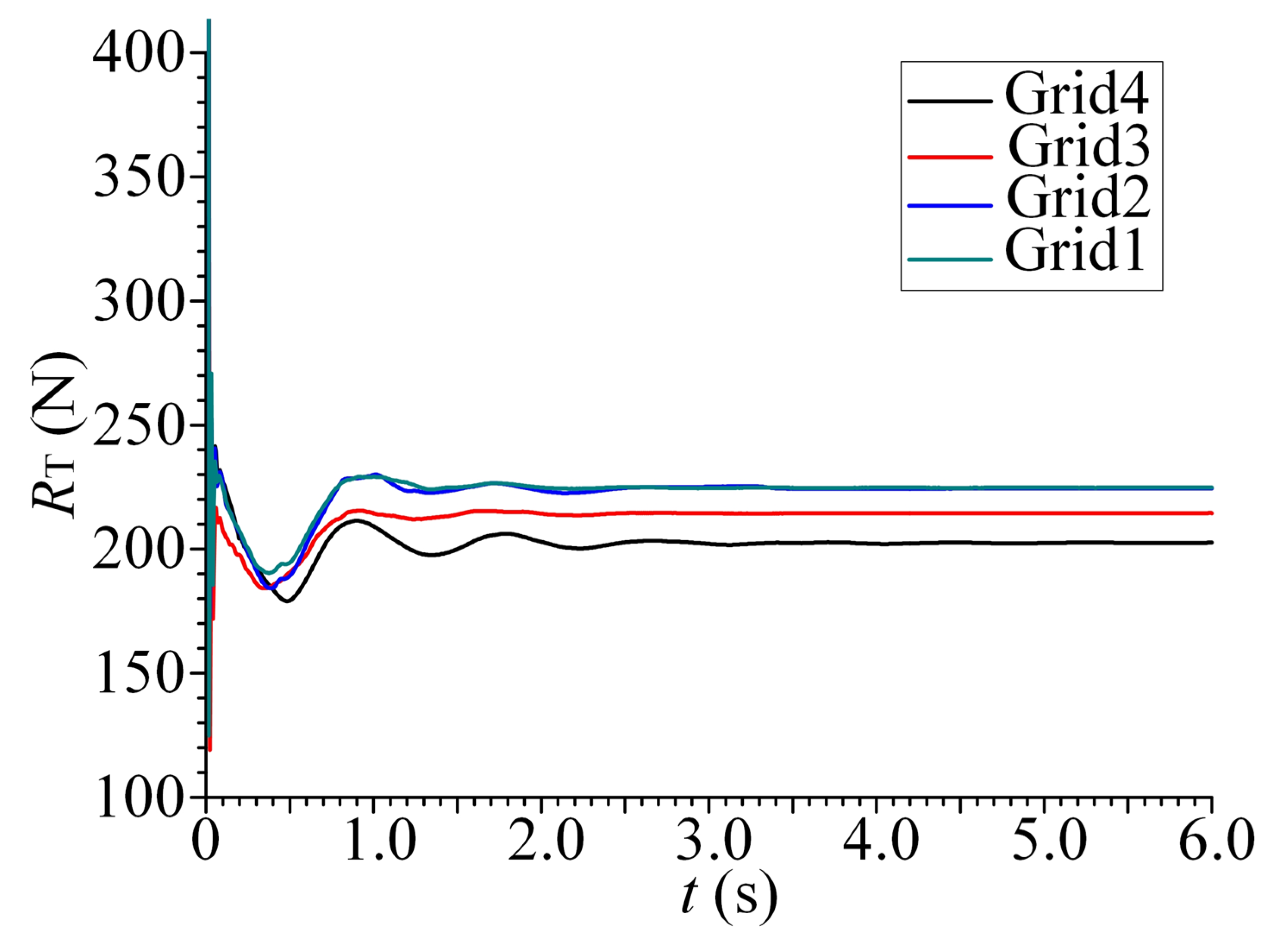
Table 4 and Figure 11 indicate that the resistance curves of the four grids have good convergence; comparing the numerical results of the four grids, the coarse grid 4 had a larger deviation compared with test results, and as the grid was refined, the deviation gradually decreased. However, when the grid was fine enough (grid 2), the further refinement of grid 1 did not greatly improve the simulation accuracy; inversely, the calculation efficiency dropped significantly due to too many grids.
Summing up the above, considering the high accuracy and the less computing time at the same time, the parameters of grid 2 were selected to be the more suitable grid input setting, and subsequent grid settings were all based on grid 2.
4.2. Y+ Values
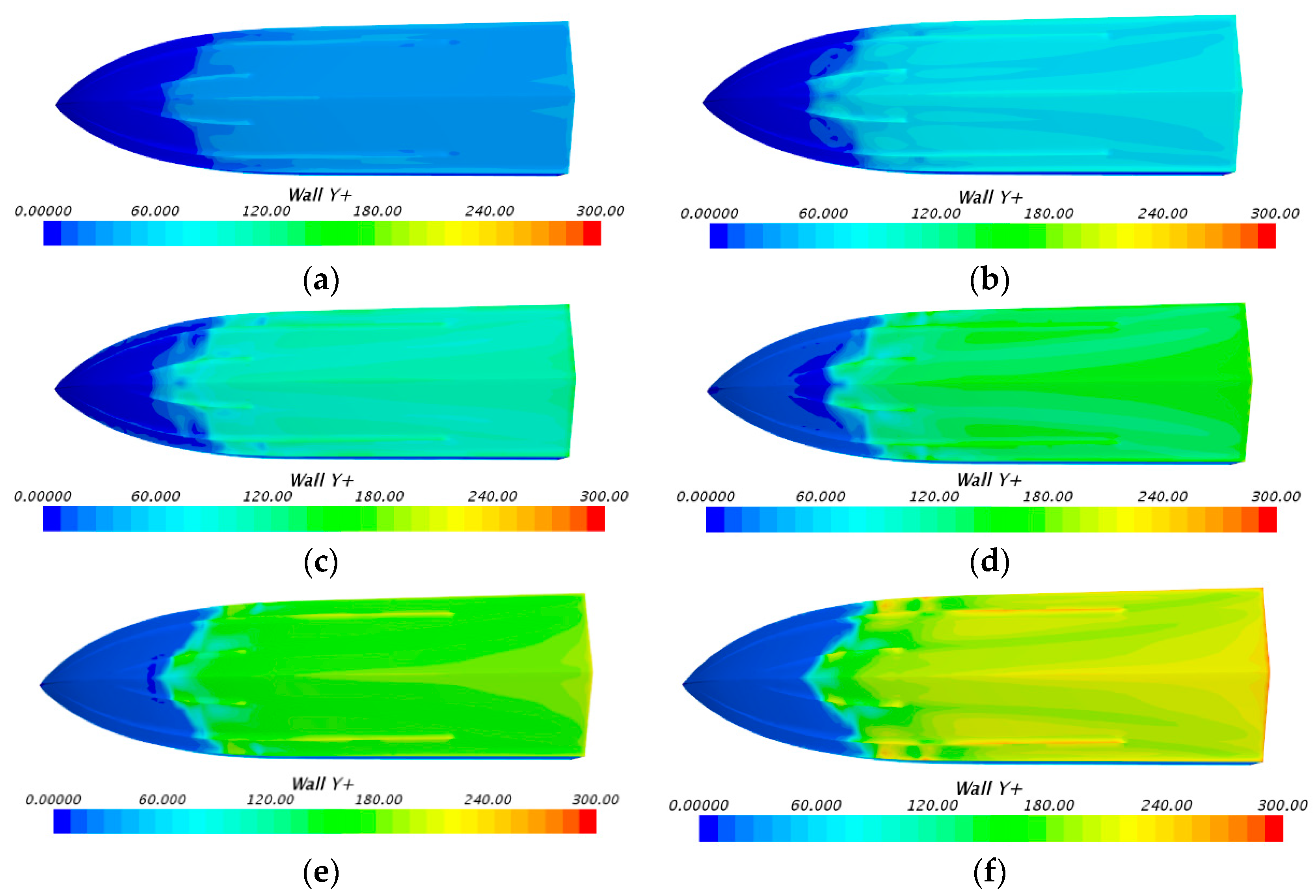
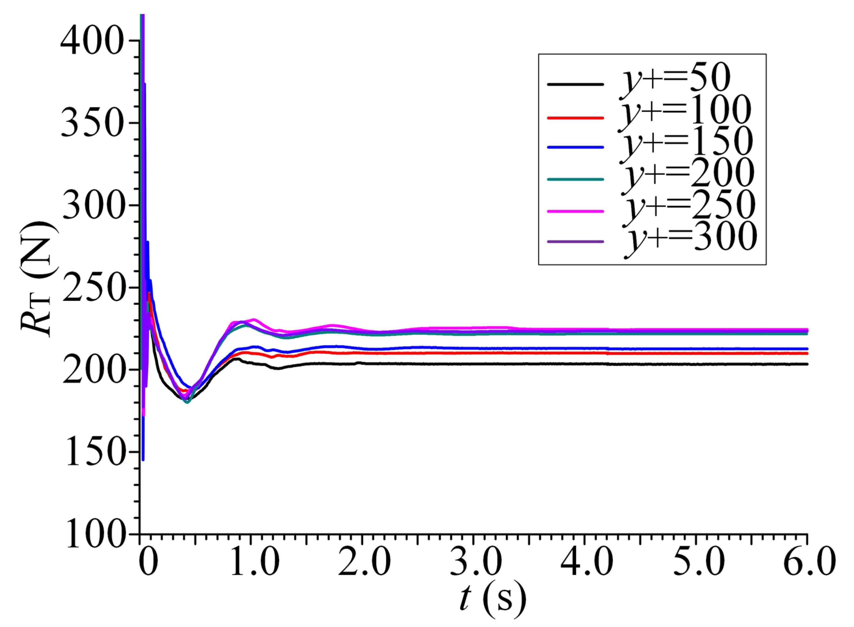
In general, the value of y+ has a profound influence on the calculation accuracy. In 2005, Wang et al. [39] analyzed the influence of y+ on the turbulence problem, indicating that the y+ value near the hull should be restrained between 30 and 300. Thus, to ascertain the influence of y+ value on the calculation accuracy, six different y+ values of 50, 100, 150, 200, 250, and 300 were selected, and as in the previous CFD set up, simulations of different y+ values were conducted, and the wall y+ and resistance after calculation were obtained, which are shown in Figure 12 and Table 5, respectively.
Figure 12 indicates that the setting of boundary layer under different y+ values was reasonable, and the amount waterline of the vessel arose changed due to the increase of the trim angle; the reduction of the waterline length made the y+ value less than the theoretical value.
Table 5 and Figure 13 indicate that the resistance curves of different y+ values had the same convergence. However, a smaller y+ value made the calculation deviation larger due to the sharp reduction of the waterline length. When y+ = 250, the deviation was smallest, so subsequently, the y+ value of 250 was adopted in this research.
4.3. Time Step of Iteration
The determination of time step (∆ts) is usually based on the incoming flow characteristics, and it must satisfy not less than the distance of the designed minimum grid at the same time. Thus, with the aim of high accuracy and solution efficiency, the influence of the ∆ts on the deviation was analyzed in this section.
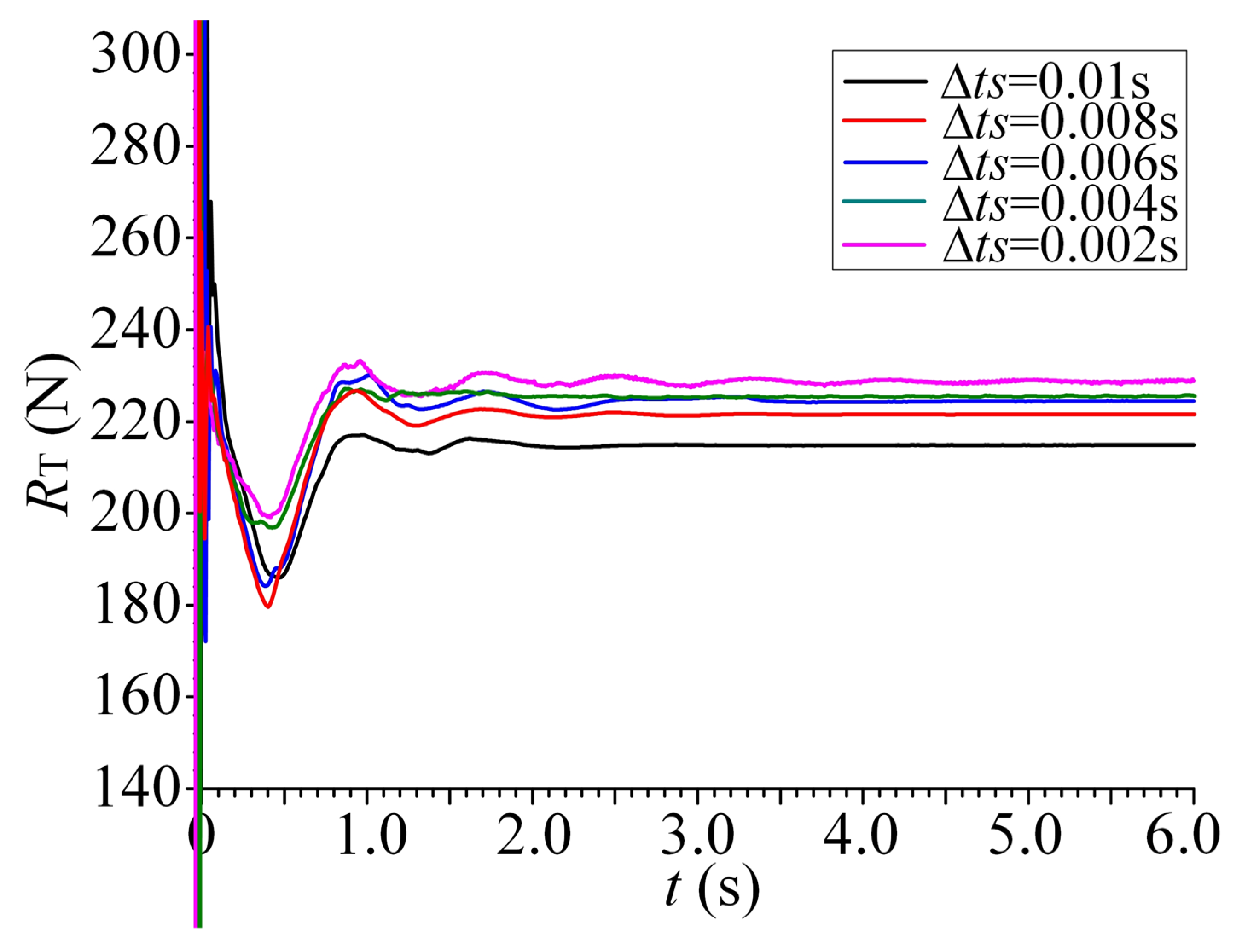
To ascertain the appropriate value of ∆ts, five values of 0.01 s, 0.008 s, 0.006 s, 0.004 s, 0.002 s were used to compute the resistance, and the numerical results of different ∆ts values were compared with the test, and are presented in Table 6 and Figure 14.
Table 6 and Figure 14 shows that the five resistance curves had the same convergence trend, the larger ∆ts (0.01 s) had a weaker calculation accuracy, and the deviation became smaller with the shortening of the time step, which indicates a smaller time interval is conducive to improve the solution precision. However, when the ∆ts was less than 0.004 s, further reducing the ∆ts value greatly increased the convergence duration, which caused a waste of calculation efficiency, so the time step ∆ts = 0.004 s was adopted because of its higher accuracy and lesser calculation duration.
Summing up the above, the influences of the grid parameters, y+ values, and time step on the calculation accuracy and efficiency were verified. The results show that the numerical method had good convergence, high accuracy, and appropriate efficiency in simulating the navigation of the model in calm water.
4.4. Comparison of Numerical and Experimental Results
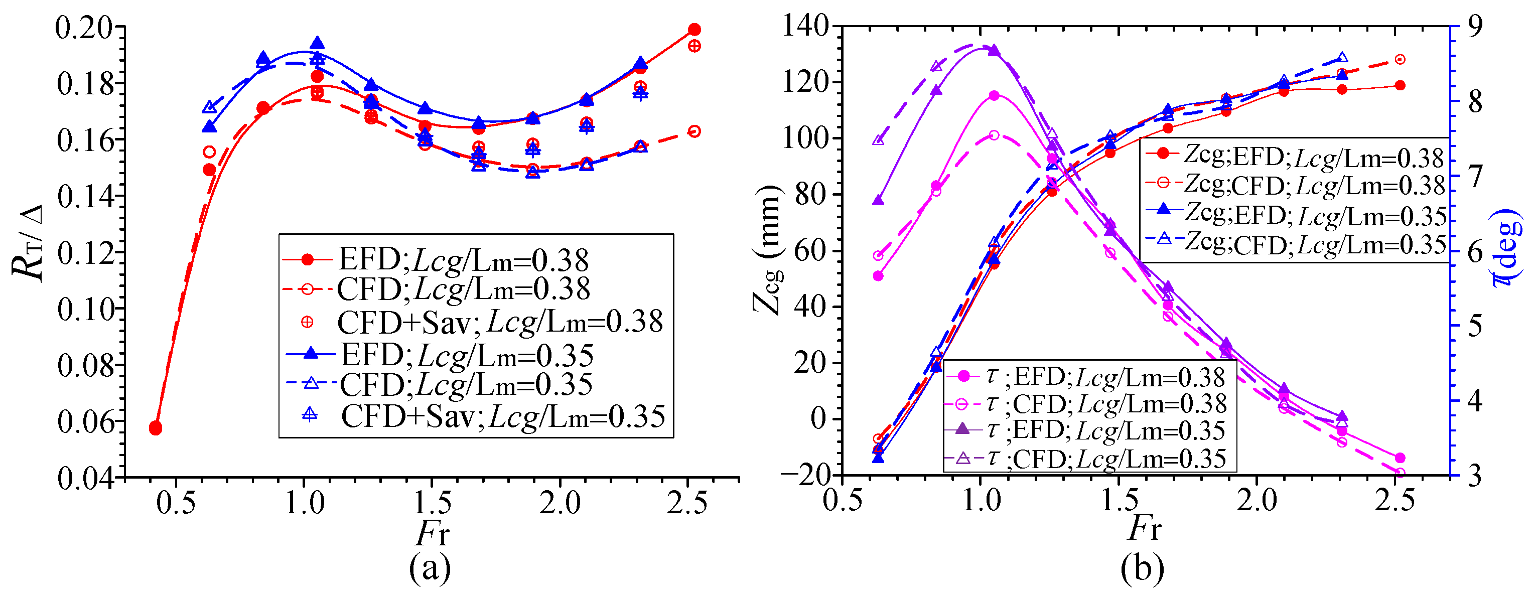
As in the aforementioned CFD setup, simulations were performed for the model at Fr =0.63–2.52 or until the porpoising appears when Lcg/Lm = 0.38 (condition two) and 0.35. The comparison between experimental data and simulated values for total resistance (RT), sinkage Zcg, and trim angle τ are shown in Figure 15, and the deviations are listed in Table 7.
Whether the ratio Lcg/Lm was 0.38 or 0.35, the changing trend of the CFD results for the RT, Zcg, and τ with speed was consistent with the test, as shown in Figure 15. During the planing stage (Fr ≥ 1.05), for the Zcg and τ when Lcg/Lm = 0.38, the maximum deviations were 10.06% and −6.6%, respectively; when Lcg/Lm = 0.35, the maximum deviations were 10.42% and −4.87%, respectively, most deviations of the remaining were below 10%, as shown in Table 6, that indicates the CFD setup could accurately forecast the sailing attitudes (Zcg and τ) of the model in the planing regime. But for the Zcg and τ in the draining state (Fr < 1.05), the deviations of Zcg were relatively larger, the deviations of τ were smaller, controlled at approximately 12% or lower.
In addition, for the computation of RT in the draining and semi-planing state (Fr ≤ 1.05), the deviations were controlled below 5%, which implies that the CFD setup had better forecast precision for the RT at that stage. However, when entering the planing state, as speed increased, the deviations of RT under the two conditions got larger, especially at Fr = 2.52 when Lcg/Lm = 0.38, the maximum deviation attained was 18.15%, which indicates the numerical method could weakly forecast the RT of the model during the high-speed planing stage (Fr > 2.1). In this stage, the spray resistance accounted for a large proportion of the total resistance, but the size of the refined mesh was unable to finely capture the tiny splash and jet. Concurrently, the nonlinear factors such as splash and jet were not effectively solved by the turbulence model, which caused the forecast precision to descend.
To obtain more accurate results of the RT during the high-speed planing stage, based on the trim angle obtained by the CFD method and combining the whisker spray equation reported by Savitsky [27], the spray resistance (RS) was computed and further added to the RT solved by the CFD method, the amendatory RT are summarized in the brackets of the third column in Table 7 and Figure 15a. Comparing the amendatory RT with test results, the maximum deviation was −6.53% at Fr = 1.89 when Lcg/Lm = 0.35, which proves the calculated results of the RT could be remarkably improved after the correction of the whisker spray equation of Savitsky [27].
In addition, under conditions two and three, porpoising respectively occurred at v = 13 m/s and 12 m/s in the simulation process, which accorded with the observed phenomena during the test. In brief, the combination of the CFD method and the whisker spray equation of Savitsky [27] achieved good forecasting of the total resistance and sailing attitude of the vessel during the high-speed planing stage.
5. Results and Discussion
5.1. Side-Hulls Inhibition of Porpoising Instability in High-Speed Crafts
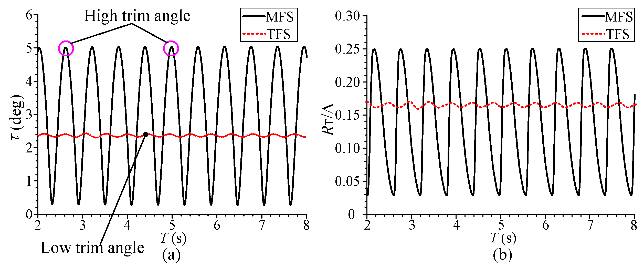
To verify that the release of side-hulls can inhibit porpoising instability in high-speed crafts, simulations for the initial designed TFS (Table 1) advancing in calm water at Fr = 2.73 (condition two) and 2.52 (condition three) were performed, and the oscillation curves with time of τ and RT were attained. Based on the previous computations of the MFS, the oscillation comparisons of the τ and RT in the MFS and TFS were conducted; the results under condition two are presented in Figure 16.
The τ and RT of the TFS exhibited minimal oscillation, but that of the MFS was significant, which indicates that the side-hulls could effectively inhibit porpoising instability.
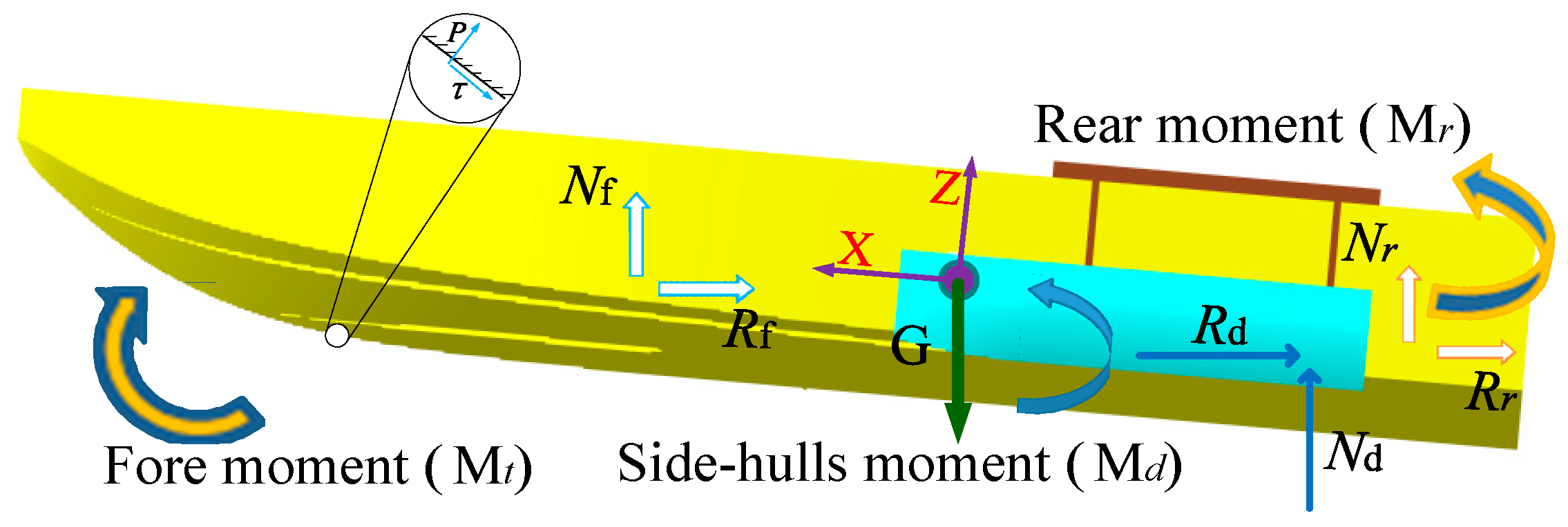
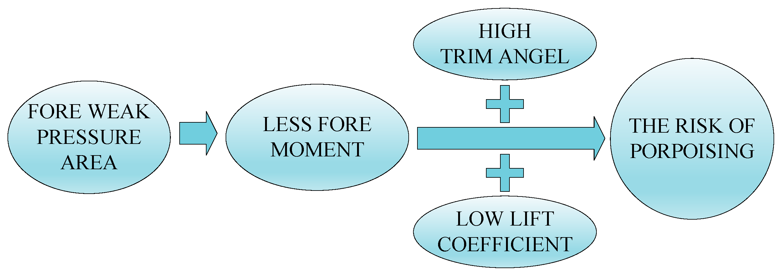
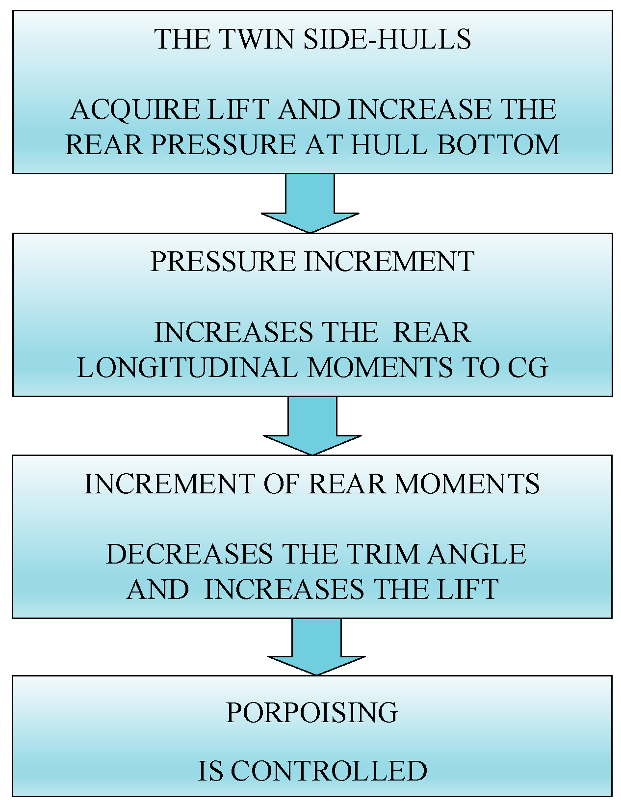
To ascertain why porpoising occurs, the pressure distributions of the hull bottom in the MFS and the TFS were compared, and results are shown in Figure 17. A weak pressure area arose at the fore of hull bottom in the MFS, indicating that the fore moment Mf (Figure 18) was relatively less than that of the rear moment Mr, and due to the high trim angle (Figure 16a) and low lift coefficient, porpoising occurred, the specific cause of this are explained in Figure 19.
When porpoising occurred, releasing the twin side-hulls into water caused them to acquire more lift and longitudinal moment Md to the CG, which is equivalent to increasing the lift of hull bottom and the rear longitudinal moment Mr to the CG; thus, the higher trim angle was decreased (Figure 16a). A strong pressure area arises at the fore of the hull bottom, so the porpoising was inhibited, the detailed explanation is shown in Figure 20.
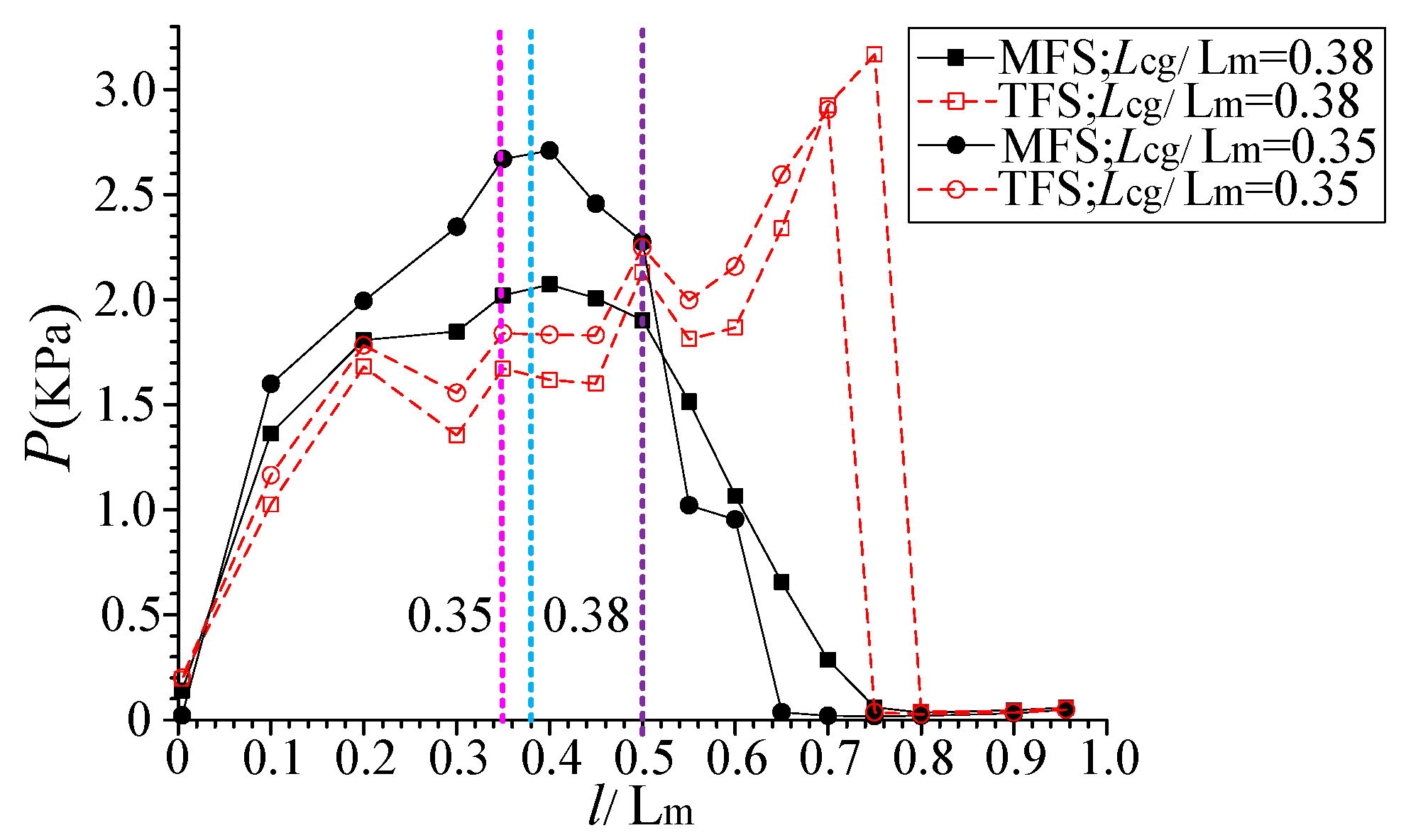
When porpoising occurs in the MFS and TFS, the pressure from stern to bow on the keel line was acquired by using probe technology; the results are summarized in Figure 21. For the MFS, the maximum pressure mainly concentrated near the CG; when the location ratio l/Lm exceeded 0.5, the pressure at the fore area reduced sharply, which led to porpoising. Conversely, for the TFS, most of the maximum pressure was located in the fore area (l/Lm > 0.5), and the pressure at the CG and rear was relatively lower, which further explains the inhibition of the side-hulls on porpoising.
5.2. Influence of Side-Hulls on Sailing Attitudes and Hydrodynamic Performance at Different Speeds
In this section, adopting the same CFD setup and the whisker spray equation of Savitsky [27], computations for the initial designed TFS (Table 1) sailing at different speeds were carried out, and the influence of the side-hulls on sailing attitudes and hydrodynamic performance were analyzed. The dimensionless resistance (CT = RT/∆) and sailing attitudes at different speeds in the MFS and TFS when Lcg/Lm = 0.38 are shown in Figure 22.
Figure 22a shows that the RT of the boat in the TFS was larger when crossing the resistance peak, and during the high-speed planing stage, the RT in the TFS was relatively larger than that in the MFS at an equal speed, indicating releasing the side-hulls into the water could bring more resistance when porpoising. For the main hull resistance RM in the TFS, the changing trend with increasing speed was similar to the MFS, and when Fr > 1.89, the RM even surpassed its previous resistance peak value.
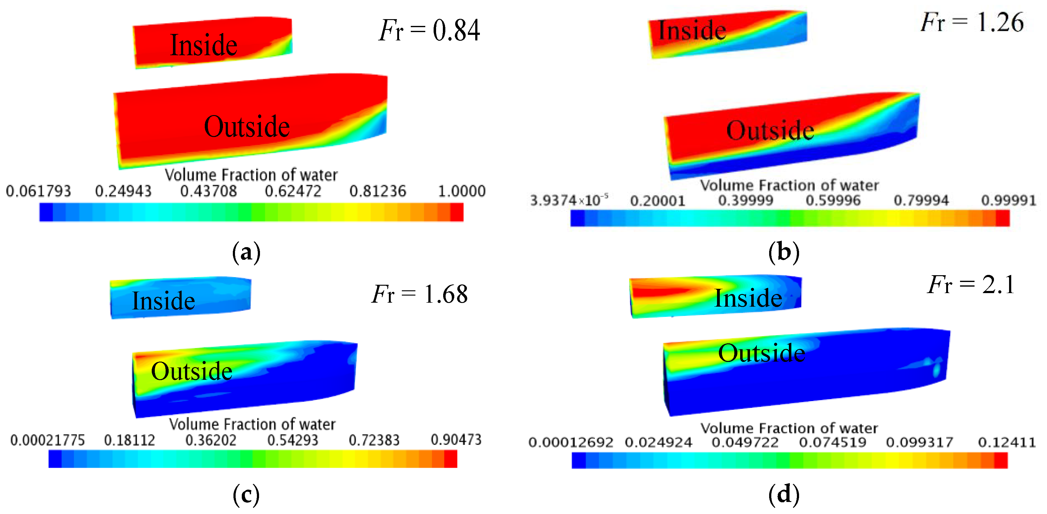
In addition, Figure 22b shows in any navigation stage, the trim angle in the TFS was smaller than that of the MFS at equal speeds, especially during the draining stage, the discrepancy was more obvious. The sinkage of TFS in the draining stage was larger compared with the MFS; however, during the planing stage, the sinkage of the MFS was relatively larger. This was mainly because most of the volume of the side-hulls was submerged into the water during the draining stage; the side-hulls could acquire more lift and lead to the further lifting of the CG. When entering the planing stage, the side-hulls were gradually lifted out of the water with increasing speed, as shown in Figure 23; the reduction of side-hulls immersion volume made them acquire less lift, which is mainly used to generate more rear moment to adjust the trim angle; only a fraction of the lift is used to raise the CG of craft.
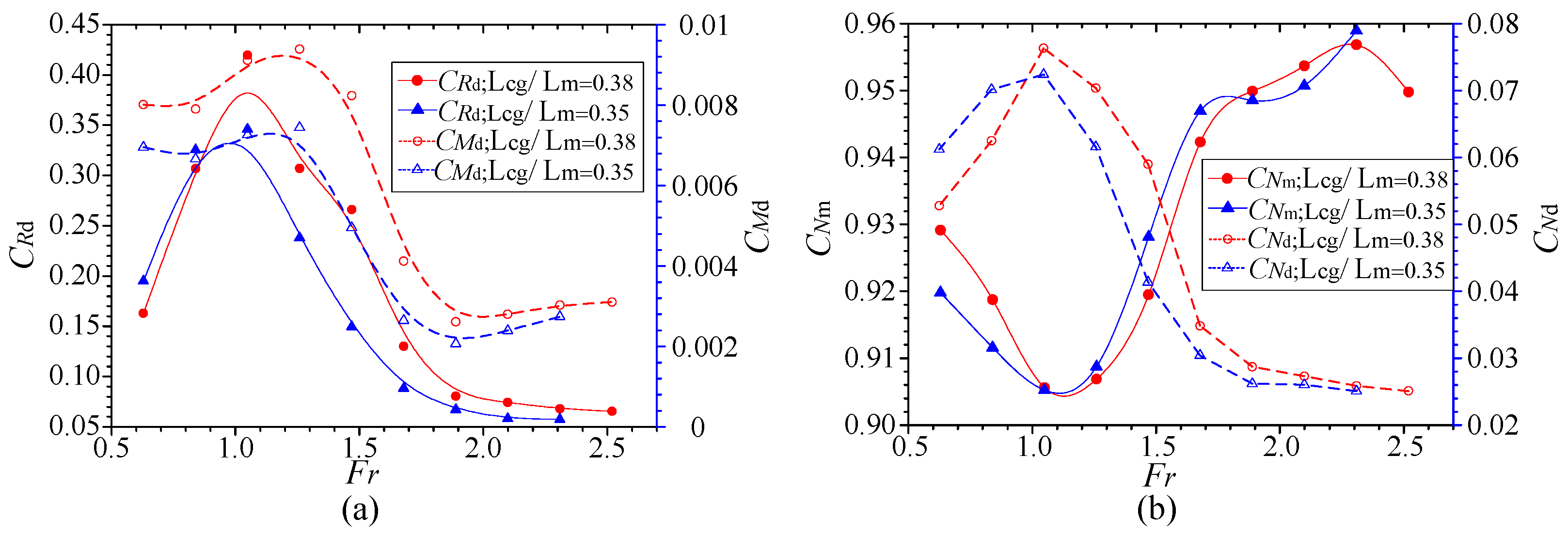
Figure 24a presents the change with speed of the side-hulls resistance (Rd) and the moment of side-hulls to the CG (Md), which shows the Rd and Md gradually increased with the increase of speed during the draining stage, but when entering the planing stage, both the Rd and the Md had a significant decline due to the reduction of the side-hulls immersion volume; but when Fr > 1.89 the Md increased as speed further increased, indicating porpoising could be inhibited by the side-hulls.
Moreover, Figure 24b shows that the changing trend of the side-hulls lift (CNd) was consistent with that of the CMd. For the main hull lift (CNm) in the TFS, with the increase of speed the CNm reduced during the draining stage; but when entering the planing stage, the CNm exhibited an obvious rise; when Fr > 1.89, the upward trend gradually slowed.
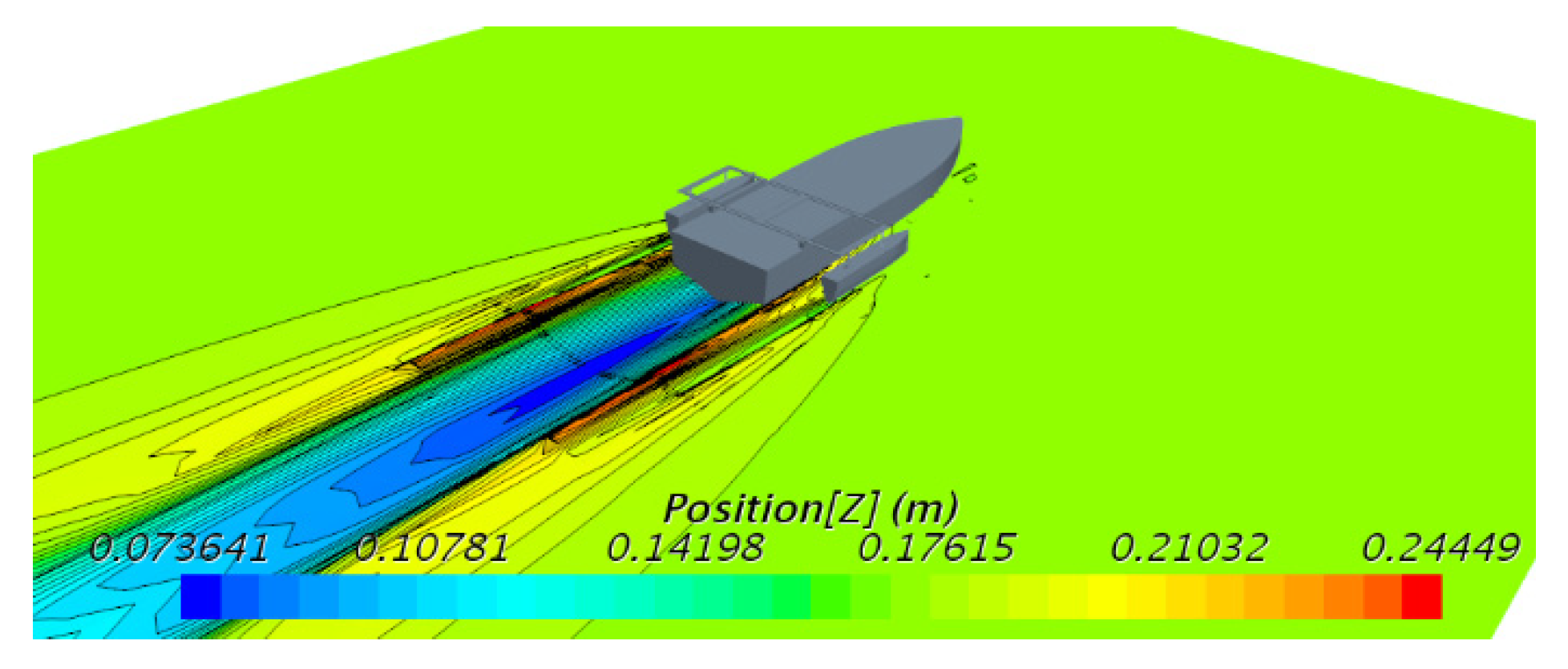
Figure 25 shows the free surface of the vessel in the TFS when porpoising; we observed that the main hull was lifted very high due to the strong hydrodynamic lift during the high-speed planing stage. At the same time, only the rear part of the side-hulls was slightly immersed in the water, so the interference influence on the side-hulls, caused by the ship traveling wave of the main hull, was lesser, the wave surface change mainly concentrated on the stern wake.
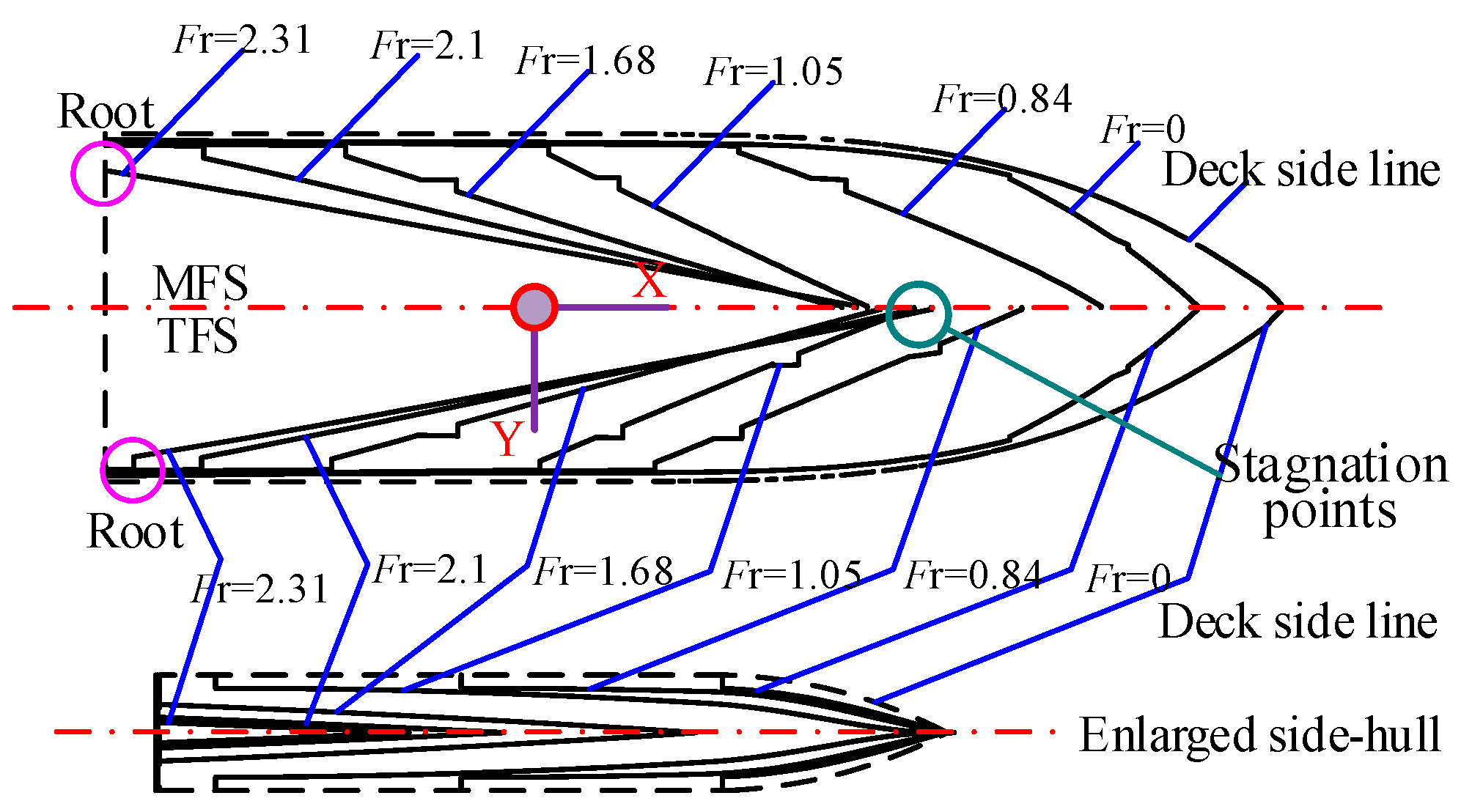
Based on the attained Zcg and τ values, the waterline surfaces (WS) of the two navigation states at different speeds were intercepted and compared utilizing the Creo software; the results are shown in Figure 26. As the speed increased, the root of the WS gradually moved backward to the stern, and the WS became sharper and longer; the area of WS also decreased, causing porpoising. However, the release of side-hulls delayed the backward movement of the root, lengthened the WS, and the stagnation points moved forward even far beyond the MFS, which further enhanced the longitudinal stability during high-speed navigation.
5.3. Influence of Longitudinal and Vertical Side-Hull Locations on Inhibiting Porpoising
The longitudinal and vertical locations of the side-hulls had a profound impact on porpoising instability. To simulate the location adjustments of twin side-hulls in the two directions, we chose the TFS, whose side-hulls were installed at at = 0.23 m, bt = 0.548 m and ct = 0.07 m (No. 3 in Table 8) as the basic research object.
5.3.1. Location Adjustments of the Twin Side-Hulls
Figure 27 shows the side-hulls adjustment mode of the longitudinal location. The ratio a/Lm was adjusted and the longitudinal location of side-hulls, the Lcg, and the longitudinal inertia tensor (Iyt) of the TFS were changed. Then, six different longitudinal locations of the side-hulls are designed and shown in Figure 28a, corresponding to the NOs. 1–6, as listed in Table 8. Besides, for condition two, the Lcg and Iyt of the TFS after adjustment was measured by utilizing the Creo software, presented in Table 8.
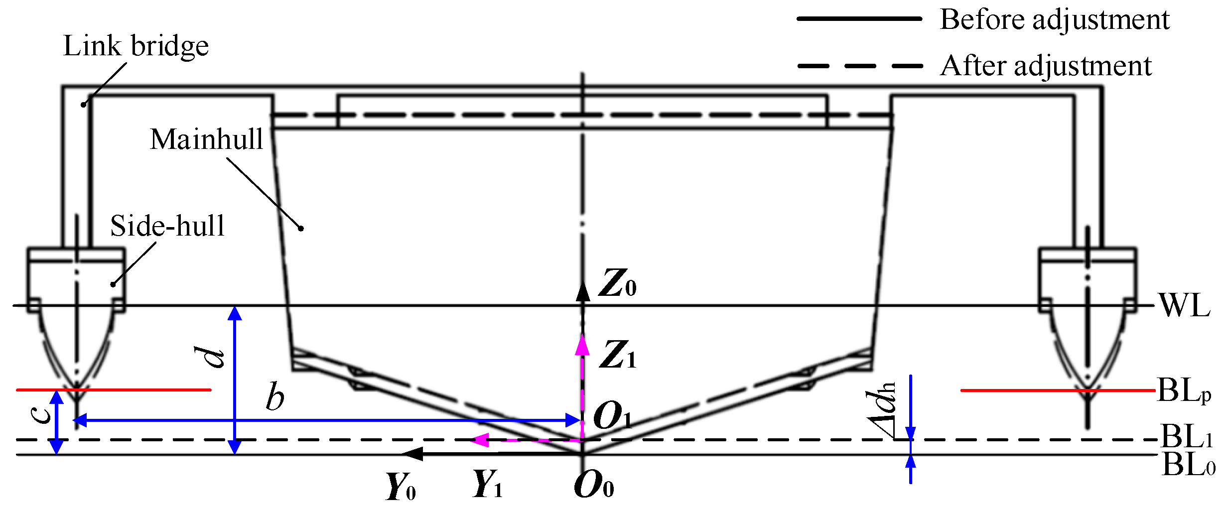
Figure 29 shows the vertical adjustment mode of the twin side-hulls, in which the solid and dashed lines separately represent the two positions before and after adjustment, d represents the waterline position relative to the Base line (BL) of the main hull, c is the distance between main hull BL and demihull BL, ∆dh represents the variation of BL position for the main hull before and after adjustment. Six different vertical locations of the side-hulls were obtained, shown in Figure 28b, corresponding to the six draft ratios Dd/Tm (NOs. 1–6) listed in Table 9, where Sm and Sd represent the waterline (WL) areas of the main hull and twin side-hulls, respectively.
5.3.2. The Optimal Range of Side-Hull Locations on Porpoising Instability
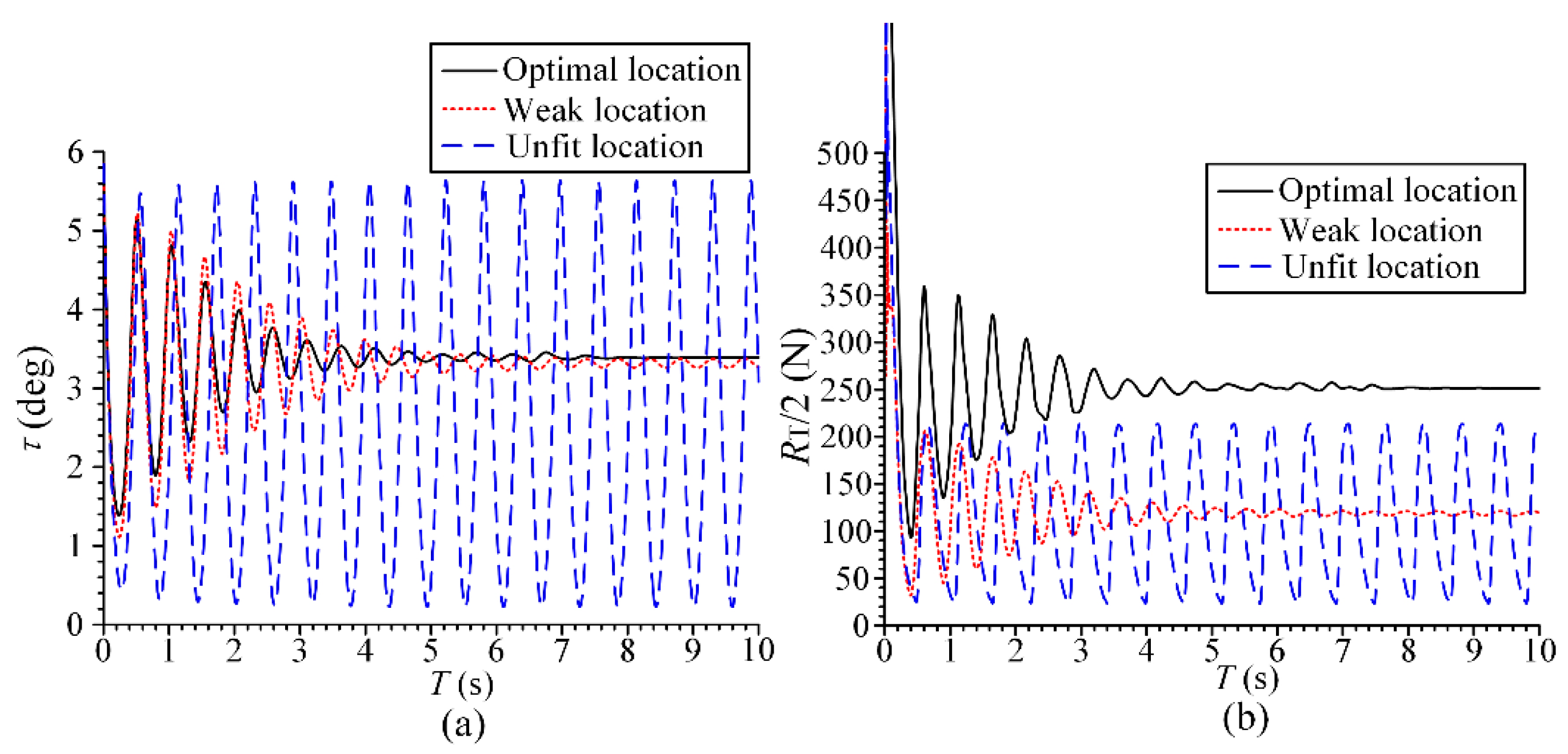
To achieve the inhibition of porpoising at the cost of lower resistance, the RT and τ in the TFS with different side-hulls longitudinal and vertical locations were computed, and the positive location ranges are presented in this section. Moreover, to evaluate the inhibition effect on porpoising, the dimensionless oscillation amplitude of trim angle (Cτ = |τ-τav|/τav) and the average resistance (CRa = Rav/∆) were introduced. As shown in Figure 30, for the Cτ prescribing that when the side-hulls were at the optimal location (Cτ < 2%), the porpoising was completely inhibited; at the weak location (2% < Cτ < 10%), the craft was regarded as achieving the stable navigation; at the unfit location (Cτ > 10%), porpoising occurred; for the CRa prescribing when CRa < CRa _m (Rav_m/∆), the side-hulls were at the optimal location, here the Rav_m is the average resistance of the MFS when porpoising; when CRa _m < CRa < 1.5 CRa _m the craft suffered more navigation resistance; when CRa > 1.5 CRa _m, sailing forward in the TFS required too much thrust and was uneconomical.
According to the six longitudinal locations (Nos. 1–6 in Table 8) and the six vertical locations (Nos. 1–6 in Table 9) of side-hulls in the TFS, adopting the spatial sampling method of full factor design [40], simulations for the TFS with 36 different side-hull locations under condition two were performed, and the results are shown in Table 10.
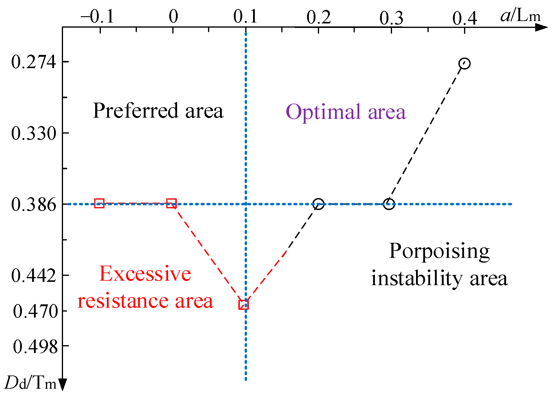
Table 10 shows with the backward movement of side-hulls, the probability that porpoising could be entirely suppressed increased. However, when the side-hulls were too backward (a/Lm = −0.1–0.1), along with an increasing draft, the average resistance Rav also increased, and when draft ratio Dd/Tm exceeded 0.442, the craft frequently suffered too much resistance, which inversely consumes more thrust. In addition, when side-hulls were relatively forward (a/Lm = 0.2–0.4) and the draft ratio exceeded 0.442, the probability that porpoising would occur, increased significantly. The more forward location (a/Lm = 0.4) is not recommended owing to the significant risk of porpoising. Considering the Cτ and CRa, the draft of the side-hulls is not recommended to exceed the ratio (Dd/Tm) of 0.442.
Summing up the above, the positive range of the side-hull location was and . As shown in Figure 31, in the preferred area, the craft could bear slightly more resistance and sail stably, while in the optimal area, porpoising was suppressed, and the boat could sail in the sea with lesser resistance.
Figure 32a shows that side-hulls being placed relatively forward (a/Lm = 0.4) was not conducive to inhibiting porpoising. For the side-hulls, when backward relative to the CG of the main hull, the deeper the draft in the vertical direction, and the greater the total resistance (Figure 32b), then the side-hulls resistance and the ratio of Rd to RT also increased when porpoising.
Figure 32e shows that when a/Lm > 0.3, the CMd becomes negative, porpoising occurs at the unfit location (Figure 32a); as the side-hulls move backward, there was an obvious increase in CMd, which further proves the previous analysis.
Figure 32f shows the more backward locations of the side-hulls relative to the CG of the main hull was more conducive to the increase of the side-hulls lift due to the planing attitudes; however, the influence of the side-hull draft on its lift was somewhat messy.
5.4. Inhibition of the Side-Hulls on the Porpoising of Real Ship with Scale Effect
To determine the impact at the scale of a real ship (RS) of the side-hulls being located in the positive range on restraining porpoising with a lesser resistance cost, the RS model (scaling λ = 2.5) in the MFS and TFS (cases 1–4 in Table 11) when porpoising were simulated, and the total resistance RT, effective power Pw curves with speed increasing of the RS were also offered in this section.
Considering higher solution cost caused by enlarged computational domain and the model, the grid parameters in Section 4.1 were enlarged in proportion to the λ, and boundary layer grids were further refined to ensure the consistency of y+ on the hull surface. Then, as in the previous CFD setup, computations for the MFS and cases 1-4 were completed.
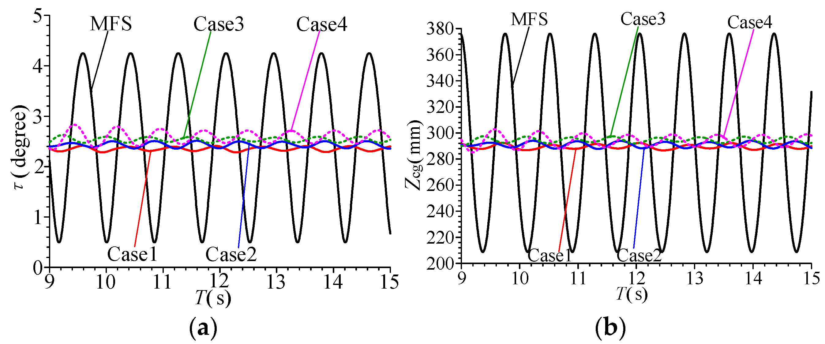
The oscillation comparisons of τ and Zcg are shown in Figure 33, further processing the results, the dimensionless oscillation amplitudes of trim angle and sinkage (CZ = |Zcg − Zav|/Zav) were attained, and based on the acquired τav, τ (maximum), and the whisker spray equation of Savitsky [27], the total resistance (Rav) including RS, the maximum resistance (Ram) and the percentage of resistance increment (PRI = (Rav − Rav_m)/Rav_m%) on releasing side-hulls when porpoising were solved and listed in Table 12.
Figure 33 shows that on the scale of a real ship, releasing the side-hulls in the positive range could significantly reduce the pitch and heave oscillation when porpoising, and the oscillation amplitudes of the more forward side-hulls placement (case 4) were larger compared with cases 1–3. Table 12 further shows the more backward side-hulls placement brought a greater resistance increment, especially for case 1, the PRI attained was 27.04%, so to avoid increasing too much resistance of RS, longitudinally, it is recommended not to have a ratio less than a/Lm = 0.1.
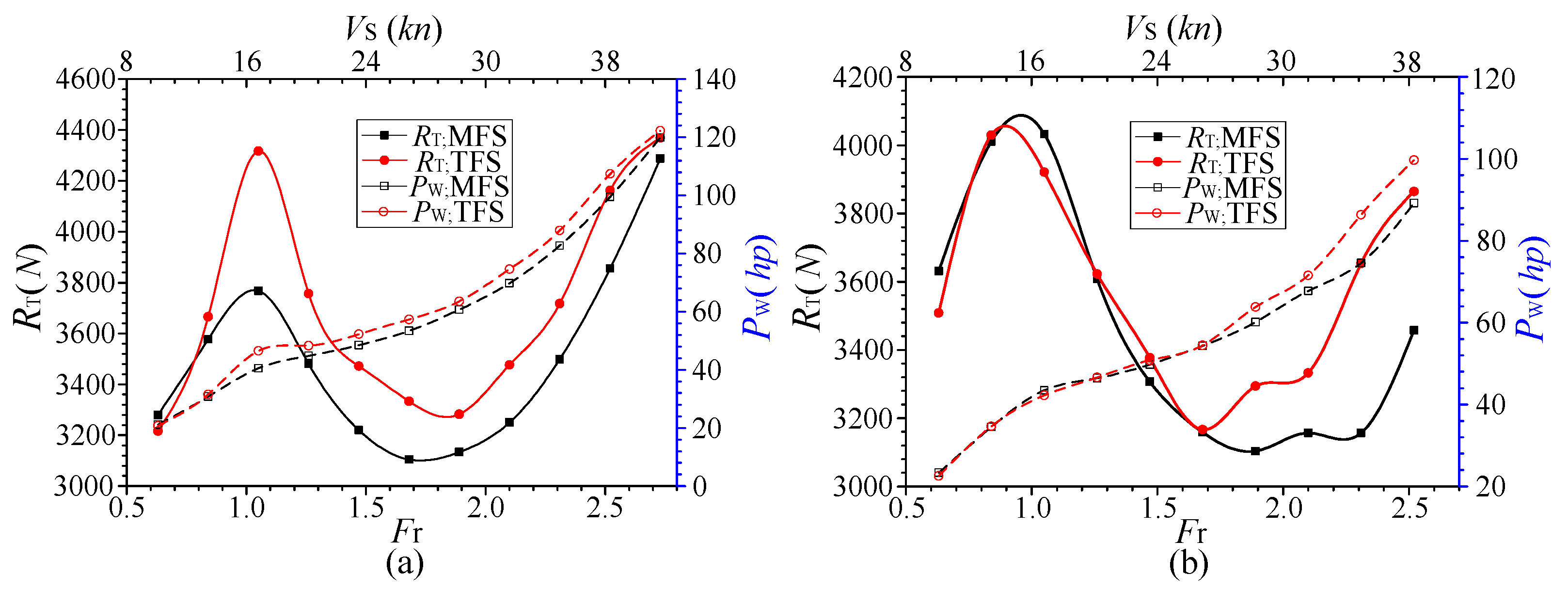
In addition, through the deliberation to Cτ, Rav, and Ram in Table 12, case 2 was chosen as the better side-hulls placement. And utilizing the verified CFD method and the whisker spray equation of Savitsky [27], RT and Pw of the RS in the MFS and TFS (cases 2) at different speeds were computed, the RT and Pw curves with speed increasing under conditions two and three, are shown in Figure 34, which can provide a sufficient reference for the overall design of planing boats with this concept.
6. Conclusions
In this study, the hydrodynamics of twin side-hulls and their inhibiting effect on the porpoising of planing boats were analyzed. Based on the CFD method, the whisker spray equation of Savitsky [27], and the test, a comparative analysis was conducted on the hydrodynamic performance of the vessel in the MFS and TFS. The optimal location range of the side-hulls for porpoising inhibition and lesser resistance was also provided.
The CFD setup can accurately forecast the sailing attitudes of the model during the planing regime, but the forecastability of the total resistance during the high-speed planing stage was weaker. The application of the whisker spray equation of Savitsky [27] allowed the deviations of amendatory resistance to be controlled within 7%, which indicates the calculation method utilized in this research could effectively forecast the total resistance, including spray resistance and sailing attitude of the vessel during the high-speed planing stage.
The weak pressure area at the fore of hull bottom in the MFS causes the fore moment to be lesser than the rear moment, coupled with the existence of high trim angle and the low lift coefficient, porpoising occurs. Releasing the side-hulls in the water increased the total lift of the hull bottom and the rear longitudinal moment; thus, the high trim angle could be decreased, and a strong pressure area at the fore inhibited porpoising instability.
The comparisons of the MFS and TFS show that releasing the side-hulls into the water was conducive to inhibiting porpoising, but sailing in the TFS yields more navigation resistance when crossing the resistance peak and during the high-speed planing stage. In addition, at any stage, the trim angle of TFS was smaller compared with the MFS at equal speeds, and the sinkage of the TFS in the draining stage was larger, but during the planing stage, that of the MFS is relatively larger.
Side-hull longitudinal locations exceeding the ratio of a/Lm = 0.3 are not recommended, and vertically, the draft ratio (Dd/Tm) is suggested not to exceed 0.442. The positive range of side-hull locations is and , and in the optimal area, porpoising could be suppressed; the boat can also then sail with lesser resistance. In addition, at the scale of a real ship, longitudinally, the side-hull locations are recommended not to be less than the ratio a/Lm = 0.1 to avoid increasing resistance.
Author Contributions
Conceptualization, Y.S. and J.W.; methodology, J.W.; software, J.W. and X.B.; validation, X.B., J.W. and Y.S.; formal analysis, J.W.; investigation, J.W.; resources, J.Z.; data curation, X.B.; writing—original draft preparation, J.W.; writing—review and editing, J.W. and J.Z.; visualization, J.Z.; supervision, Y.S.; project administration, Y.S.; funding acquisition, J.Z. All authors have read and agreed to the published version of the manuscript.
Funding
The research reported here was supported by the National Natural Science Foundation of China (Grant No. 52071100). The authors would like to express their gratitude to all the test participants for their suggestions and observations that helped in improving the present research.
Data Availability Statement
Data is contained within the article.
Conflicts of Interest
The authors declare no conflict of interest.
References
- Yasin, M.; Amir, H.N. Drag Optimization of a planing vessel based on the stability criteria limits. China Ocean Eng. 2019, 33, 365–372. [Google Scholar]
- Yasin, M.; Amir, H.N. Comparison of numerical solution and semi-empirical formulas to predict the effects of important design parameters on porpoising region of a planing vessel. Appl. Ocean Res. 2017, 68, 228–236. [Google Scholar]
- Shuo, W.; Yumin, S.; Yongjie, P.; Huanxing, L. Numerical study on longitudinal motions of a high speed planing craft in regular waves. J. Harbin Eng. Univ. 2014, 35, 45–52. [Google Scholar]
- Clement, E.P.; Blount, D. Resistance tests of systematic series of planing hull forms. Trans. Soc. Nav. Archit. Mar. Eng. 1963, 71, 491–561. [Google Scholar]
- Blount, D.L.; Codega, L.T. Dynamic stability of planing boats. Mar. Technol. 1992, 29, 4–12. [Google Scholar]
- Katayama, T.; Teshima, A.; Ikeda, Y. A Study on transverse proposing of a planning craft in drifting motion. J. Mar. Sci. Appl. 2001, 236, 181–190. [Google Scholar]
- Payam, L.; Mahmud, A.; Reza, K.E. Numerical investigation of a stepped planning hull in calm water. Ocean Eng. 2015, 94, 103–110. [Google Scholar]
- Reza, K.E.; Mohammad, A.R.; Sajad, H. Hydrodynamic evaluation of a planing hull in calm water using RANS and Savitsky’s method. Ocean Eng. 2019, 187, 106–221. [Google Scholar]
- Savitsky, D. Chapter IV planning craft of modern ships and craft. Naval Eng. 1985. Special Edition. [Google Scholar]
- Najafi, A.; Siamak, A.; Mohammad, S.S. RANS simulation of interceptor effect on hydrodynamic coefficients of longitudinal equations of motion of planing catamarans. J. Braz. Soc. Mech. Sci. Eng. 2015, 37, 1257–1275. [Google Scholar] [CrossRef]
- Jokara, H.; Zeinali, H.; Tamaddondar, M.H. Planing craft inhibition using pneumatically driven trim tab. Math. Comput. Simul. 2020, 178, 439–463. [Google Scholar] [CrossRef]
- Sayyed, M.S.; Parviz, G. Experimental and numerical analyses of wedge effects on the rooster tail and porpoising phenomenon of a high-speed planing craft in calm water. J. Mech. Eng. Sci. 2019, 233, 4637–4652. [Google Scholar]
- Mehran, M.; Antonio, C.F. The interceptor hydrodynamic analysis for inhibition the porpoising instability in high speed crafts. Appl. Ocean Res. 2016, 57, 40–51. [Google Scholar]
- Mansoori, M.; Fernandes, A.C.; Ghassemi, H. Interceptor design for optimum trim inhibition and minimum resistance of planing boats. Appl. Ocean Res. 2017, 69, 100–115. [Google Scholar] [CrossRef]
- Mansoori, M.; Fernandes, A.C. Interceptor and trim tab combination to prevent interceptor’s unfit effects. Ocean Eng. 2017, 134, 140–156. [Google Scholar] [CrossRef]
- Ahmet, G.A.; Baris, B. An experimental investigation of interceptors for a high speed hull. Int. J. Nav. Archit. Ocean Eng. 2019, 11, 256–273. [Google Scholar]
- Hongjie, L.; Zhidong, W. Real-time numerical prediction method of dolphin motion in high-speed planing crafts. J. Shanghai Jiaotong Univ. 2014, 48, 106–110. [Google Scholar]
- Hanbing, S.; Yumin, S.; Jin, Z.; Kexin, Z.; Jiayuan, Z. Longitudinal navigation performance test of high-speed unmanned boat. J. Shanghai Jiaotong Univ. 2013, 47, 278–283. [Google Scholar]
- Katayama, T.; Yoshiho, I. Hydrodynamic forces acting on porpoising craft at high speed. J. Ship Ocean Tech. 1999, 3, 17–26. [Google Scholar]
- Katayama, T.; Fujimoto, M.; Ikeda, Y. A study on transverse stability loss of planning craft at super high forward speed. Int. Shipbuilding Pro. 2007, 54, 365–377. [Google Scholar]
- Sasan, T.; Abbas, D. Mathematical simulation of planar motion mechanism test for planing hulls by using 2D+T theory. Ocean Eng. 2018, 169, 651–672. [Google Scholar]
- Parviz, G.; Sasan, T.; Abbas, D.; Zamanian, R. Steady performance prediction of a heeled planing boat in calm water using asymmetric 2D+T model. J. Eng. Mar. Environ. 2017, 231, 234–257. [Google Scholar]
- Parviz, G.; Sasan, T.; Abbas, D. Coupled heave and pitch motions of planing hulls at non-zero heel angle. Appl. Ocean Res. 2016, 59, 286–303. [Google Scholar]
- Shuo, W.; Yumin, S.; Zhaoli, W.; Xuguang, Z.; Huanxing, L. Numerical and experimental analyses of transverse static stability loss of planing craft sailing at high forward speed. Eng. App. Comput. Fluid Mech. 2014, 8, 44–54. [Google Scholar]
- Abbas, D.; Sasan, T.; Ahmadreza, K.; Khosravani, R. Numerical study on a heeled one-stepped boat moving forward in planing regime. Appl. Ocean Res. 2020, 96, 102–117. [Google Scholar]
- Yi, J. Hybrid Hydro-Aerodynamic Characteristics Investigation on High-Speed Planing Hull under the Coupling Effect of Step and Tunnel. Doctoral Thesis, Harbin Engineering University, Harbin, China, 2018. [Google Scholar]
- Savitsky, D.; Delorme, M.F.; Datla, R. Inclusion of whisker spray drag in performance prediction method for high-speed planing hulls. Mar. Technol. 2007, 44, 35–56. [Google Scholar]
- Yi, J.; Hanbing, S.; Jin, Z.; Ankang, H.; Jinglei, Y. Experimental and numerical investigations on hydrodynamic and aerodynamic characteristics of the tunnel of planning trimaran. Appl. Ocean Res. 2017, 63, 1–10. [Google Scholar]
- Florian, R.; Menter, P. Improved two-equation turbulence models for aerodynamic flows. NASA Tech. Memo. 1992, 103, 103975. [Google Scholar]
- Mireille, B.F.; Carlos, F.L.; Arman, H.; Fleck, B.A. Performance of turbulence models in simulating wind loads on photovoltaics modules. Energies 2019, 12, 3290. [Google Scholar]
- Menter, F.R. Two-equation eddy-viscosity turbulence models for engineering applications. AIAA 1994, 32, 1598–1605. [Google Scholar] [CrossRef] [Green Version]
- Ghasemi, E.; Mceligot, D.M.; Nolan, K.P.; Crepeau, J.; Siahpush, A.; Budwig, R.S.; Tokuhiro, A. Effects of adverse and favorable pressure gradients on entropy generation in a transitional boundary layer region under the influence of free stream turbulence. Int. J. Heat Mass Transfer. 2014, 77, 475–488. [Google Scholar] [CrossRef]
- Shuo, W.; Yumin, S.; Yongjie, P.; Xi, Z. Study on the accuracy in the hydrodynamic prediction of high-speed planing crafts of CFD method. J. Ship Mech. 2013, 17, 1107–1114. [Google Scholar]
- Hirt, C.W.; Nichols, B.D. Volume of Fluid (VOF) method for the dynamics of free boundary. J. Comput. Phys. 1981, 39, 201–225. [Google Scholar] [CrossRef]
- Scardovelli, R.; Zaleski, S. Direct numerical simulation of free-surface and interfacial flow. Annu. Rev. Fluid Mech. 1999, 31, 567–603. [Google Scholar] [CrossRef] [Green Version]
- Xiaosheng, B.; Hailong, S.; Jin, Z.; Yumin, S. Numerical analysis of the influence of fixed hydrofoil installation position on seakeeping of the planing craft. Appl. Ocean Res. 2019, 90, 101863. [Google Scholar]
- Xiaosheng, B.; Jiayuan, Z.; Yumin, S. Seakeeping Analysis of Planing Craft under Large Wave Height. Water Res. 2020, 12, 1020. [Google Scholar] [CrossRef] [Green Version]
- Yumin, S.; Jianfeng, L.; Dagang, Z.; Chao, W.; Chunyu, G. Review of numerical simulation methods for full-scale ship resistance and propulsion performance. Shipbuild. China 2020, 61, 229–239. [Google Scholar]
- Wang, F. Book Computational Fluid Dynamics Analysis-Theory and Application of CFD Software; Tsinghua University Press: Beijing, China, 2005; pp. 23–49. [Google Scholar]
- Guay, M. Uncertainty estimation in extremum seeking inhibition of unknown static maps. IEEE Inhib. Syst. Lett. 2021, 5, 1115–1120. [Google Scholar]
Figure 1.
Main geometric characteristics of the hull in different navigation states: (a) monomer-form state (MFS) and (b) trimaran-form state (TFS).
Figure 1.
Main geometric characteristics of the hull in different navigation states: (a) monomer-form state (MFS) and (b) trimaran-form state (TFS).

Figure 2.
Molded lines of the model: (a) main hull; (b) side-hull.

Figure 3.
Schematic diagram of the experimental setup.

Figure 4.
Photographs of the monomer-form model.

Figure 5.
Test results of the monomer-form model: (a) total resistance; (b) sinkage and trim angle.

Figure 6.
Solver procedure of the numerical method.

Figure 7.
Dimensions and boundary conditions in the domain.

Figure 8.
Detailed grid partition of the entire computational domain: (a) axis view; (b) front view; (c) vertical view; (d) partial view.
Figure 8.
Detailed grid partition of the entire computational domain: (a) axis view; (b) front view; (c) vertical view; (d) partial view.

Figure 9.
The height of the first layer grid (y) values and total thicknesses of the boundary layer grid at different speeds.
Figure 9.
The height of the first layer grid (y) values and total thicknesses of the boundary layer grid at different speeds.

Figure 10.
The four designed grids: (a) grid 4, (b) grid 3, (c) grid 2, (d) grid 1.


Figure 11.
Resistance curves of the different grids.

Figure 12.
Wall non-dimensional distance of the first layer grid (y+) after calculation: (a) y+ = 50; (b) y+ = 100; (c) y+ = 150; (d) y+ = 200; (e) y+ = 250; (f) y+ = 300.
Figure 12.
Wall non-dimensional distance of the first layer grid (y+) after calculation: (a) y+ = 50; (b) y+ = 100; (c) y+ = 150; (d) y+ = 200; (e) y+ = 250; (f) y+ = 300.

Figure 13.
Resistance curves of the different y+.

Figure 14.
Resistance curves of the different time steps.

Figure 15.
Comparison between EFD and CFD results for (a) total resistance RT and the RT added to the whisker spray resistance, (b) sinkage and trim angle.
Figure 15.
Comparison between EFD and CFD results for (a) total resistance RT and the RT added to the whisker spray resistance, (b) sinkage and trim angle.

Figure 16.
Oscillation comparisons when Lcg/Lm = 0.38: (a) trim angle; (b) total resistance.

Figure 17.
Comparisons of the hull bottom pressure in the MFS and TFS when Lcg/Lm = 0.38.

Figure 18.
Forces and moment acted on the hull surface in the TFS.

Figure 19.
Why porpoising occurs.

Figure 20.
How side-hulls inhibit porpoising.

Figure 21.
Pressure distribution from stern to bow on keel line in the MFS and TFS.

Figure 22.
Change in total resistance and sailing attitudes with speed when Lcg/Lm = 0.38: (a) total resistance; (b) sinkage and trim angle.
Figure 22.
Change in total resistance and sailing attitudes with speed when Lcg/Lm = 0.38: (a) total resistance; (b) sinkage and trim angle.

Figure 23.
Volume fraction of water for the twin side-hulls at different speeds: (a) Fr = 0.84; (b) Fr = 1.26; (c) Fr = 1.68; (d) Fr = 2.1.
Figure 23.
Volume fraction of water for the twin side-hulls at different speeds: (a) Fr = 0.84; (b) Fr = 1.26; (c) Fr = 1.68; (d) Fr = 2.1.

Figure 24.
Forces and moment acted on the hull in the TFS at different speeds: (a) resistance and moment of the side-hulls; (b) lift of the side-hulls and the main hull.
Figure 24.
Forces and moment acted on the hull in the TFS at different speeds: (a) resistance and moment of the side-hulls; (b) lift of the side-hulls and the main hull.

Figure 25.
The free surface of the vessel in the TFS when porpoising.

Figure 26.
Waterline surface comparisons of the two navigation states when Lcg/Lm = 0.35.

Figure 27.
Longitudinal adjustment mode of the twin side-hulls.

Figure 28.
Different (a) longitudinal locations; (b) vertical locations of the side-hulls in the TFS.
Figure 28.
Different (a) longitudinal locations; (b) vertical locations of the side-hulls in the TFS.

Figure 29.
Vertical adjustment mode of the twin side-hulls.

Figure 30.
The optimal, weak, and unfit locations: (a) trim angle; (b) half total resistance.

Figure 31.
Optimization of longitudinal and vertical side-hull locations on porpoising instability inhibition and resistance reduction.
Figure 31.
Optimization of longitudinal and vertical side-hull locations on porpoising instability inhibition and resistance reduction.

Figure 32.
Influence of the longitudinal and vertical side-hull locations on (a) Cτ, (b) CRa, (c) CRd, (d) Rd/RT, (e) CMd, and (f) CNd.
Figure 32.
Influence of the longitudinal and vertical side-hull locations on (a) Cτ, (b) CRa, (c) CRd, (d) Rd/RT, (e) CMd, and (f) CNd.


Figure 33.
Oscillation comparisons of (a) τ and (b) Zcg when porpoising under condition 2.

Figure 34.
The RT, power (PW) curves of the real ship in the MFS and TFS under (a) condition two, (b) condition 3.
Figure 34.
The RT, power (PW) curves of the real ship in the MFS and TFS under (a) condition two, (b) condition 3.


Table 1.
Primary geometric details of the planing hull at each navigation state.
| Main Feature | Symbol | Value |
|---|---|---|
| Monomer-form state (MFS) | ||
| Main hull length (m) | Lm | 2.3 |
| Main hull breadth (m) | Bm | 0.702 |
| Main hull depth (m) | Tm | 0.357 |
| Main hull draft (m) | Dm | 0.168 |
| Design waterline length (m) | Lwl | 2.201 |
| Original fixed location of side-hull in the longitudinal, horizontal and vertical direction (m) | am | 0.23 |
| bm | 0.38 | |
| cm | 0.26 | |
| Main hull deadrise angle (°) | θ m | 18 |
| Displacement of main hull (kg) | ∆m | 122.4/137.3 |
| Inertia tensor of main hull (kg·m2) | Iym | 40.2 (Test model) |
| Longitudinal location of center of gravity (CG) (m) | Lcg | 0.94/0.882/0.83 |
| Vertical location of CG (m) | Vcg | 0.23 |
| Trimaran-form state (TFS) | ||
| Side-hull length (m) | Ld | 0.72 |
| Side-hull breadth (m) | Bd | 0.104 |
| Side-hull depth (m) | Td | 0.155 |
| Side-hull draft (m) | Dd | 0.098 |
| Initial design location of the released side-hulls in longitudinal, horizontal and vertical direction (m) | at | 0.23 |
| bt | 0.548 | |
| ct | 0.07 | |
| Draft of TFS (m) | Dt | 0.168 |
| Displacement of trimaran (kg) | ∆t | 137.3 |
| Inertia tensor of trimaran (kg·m2) | Iyt | 49.43 |
| Longitudinal location of CG (m) | Lcg | 0.882/0.83 |
| Vertical location of CG (m) | Vcg | 0.23 |
Table 2.
Model test conditions in calm water.
| Condition | ∆m (kg) | Lcg (m) | Lcg/Lm | τ0 (°) |
|---|---|---|---|---|
| One | 137.3 | 0.94 | 0.41 | −0.4 |
| Two | 137.3 | 0.882 | 0.38 | 0.6 |
| Three | 137.3 | 0.83 | 0.35 | 1.6 |
| Four | 125.4 | 0.882 | 0.38 | 0.6 |
Table 3.
Parameters of the four grids.
| Grid Parameters | Detailed Description | Grid 4 | Grid 3 | Grid 2 | Grid 1 |
|---|---|---|---|---|---|
| Mesh number | Entire calculation domain (k) | 238 | 524 | 788 | 1550 |
| Overset region grid size | Relative minimum size (%Lg) | 2.828 | 2 | 1.414 | 1 |
| Relative target size (%Lg) | 5.656 | 4 | 2.828 | 2 | |
| Volume control region grid size | Relative grid size in the x, y, z direction (%Lg) | 11.31 | 8 | 5.656 | 5 |
| 11.31 | 8 | 5.656 | 5 | ||
| 11.31 | 8 | 5.656 | 5 | ||
| Grid size around the free surface | Relative grid size in the x, y, z direction (%Lg) | 28.28 | 20 | 14.14 | 10 |
| 28.28 | 20 | 14.14 | 10 | ||
| 2.828 | 2 | 1.414 | 1 |
Table 4.
Resistance comparisons of the test (EFD) and numerical (CFD) results for different grids.
| Grid | Resistance (N) | Deviation (%) | |
|---|---|---|---|
| EFD | CFD | ||
| 4 | 233.436 | 202.616 | −13.203 |
| 3 | 233.436 | 214.535 | −8.097 |
| 2 | 233.436 | 224.45 | −3.849 |
| 1 | 233.436 | 224.754 | −3.719 |
Table 5.
Resistance comparisons of the test and numerical results at different y+ values.
| y+ | Resistance (N) | Deviation (%) | |
|---|---|---|---|
| EFD | CFD | ||
| 50 | 233.436 | 203.321 | −12.901 |
| 100 | 233.436 | 209.901 | −10.082 |
| 150 | 233.436 | 212.742 | −8.865 |
| 200 | 233.436 | 221.456 | −5.132 |
| 250 | 233.436 | 224.45 | −3.849 |
| 300 | 233.436 | 223.521 | −4.247 |
Table 6.
The numerical results of resistance at different determination of time steps (∆ts).
| ∆ts | Resistance (N) | Deviation (%) | |
|---|---|---|---|
| EFD | CFD | ||
| 0.01 | 233.436 | 214.902 | −7.94 |
| 0.008 | 233.436 | 221.478 | −5.123 |
| 0.006 | 233.436 | 224.45 | −3.849 |
| 0.004 | 233.436 | 225.509 | −3.396 |
| 0.002 | 233.436 | 229.033 | −1.886 |
Table 7.
The comparisons of total resistance (RT), sinkage (Zcg), and trim angle (τ).
| Fr | RT(kg·F) | Zcg(mm) | τ(deg) | ||||||
| EFD | CFD (+Sav) | Deviation (%) | EFD | CFD | Deviation (%) | EFD | CFD | Deviation (%) | |
| 0.42 | 7.94 | 7.85 | −1.12 | - | - | - | - | - | - |
| 0.63 | 20.44 | 21.30 | 4.21 | −11 | −7.01 | −36.27 | 5.66 | 5.93 | 4.70 |
| 0.84 | 23.41 | 23.46 | 0.20 | 18.3 | 20.33 | 11.09 | 6.87 | 6.79 | −1.11 |
| 1.05 | 24.98 | 24.16 (24.24) | −3.27 (−2.95) | 55.1 | 60.65 | 10.06 | 8.07 | 7.54 | −6.60 |
| 1.26 | 23.82 | 22.95 (23.08) | −3.67 (−3.09) | 81 | 84.07 | 3.79 | 7.23 | 6.91 | −4.45 |
| 1.47 | 22.54 | 21.68 (22.0) | −3.81 (−2.42) | 94.8 | 99.59 | 5.06 | 6.34 | 5.97 | −5.82 |
| 1.68 | 22.45 | 20.86 (21.54) | −7.09 (−4.04) | 103.6 | 109.26 | 5.46 | 5.27 | 5.12 | −2.94 |
| 1.89 | 22.92 | 20.45 (21.67) | −10.76 (−5.44) | 109.5 | 114.17 | 4.27 | 4.66 | 4.43 | −4.90 |
| 2.10 | 23.8 | 20.75 (22.70) | −12.81 (−4.60) | 116.7 | 119 | 1.97 | 4.05 | 3.89 | −3.95 |
| 2.31 | 25.39 | 21.57 (24.47) | −15.06 (−3.62) | 117.3 | 123.15 | 4.99 | 3.59 | 3.44 | −4.18 |
| 2.52 | 27.26 | 22.31 (26.46) | −18.15 (−2.95) | 118.8 | 128.12 | 7.85 | 3.23 | 3.03 | −6.19 |
| (a) Fr = 0.42–2.52; Lcg/Lm = 0.38; when Fr = 2.73 (v = 13 m/s), the porpoising occurs. | |||||||||
| Fr | RT(kg·F) | Zcg(mm) | τ(deg) | ||||||
| EFD | CFD (+Sav) | Deviation (%) | EFD | CFD | Deviation (%) | EFD | CFD | Deviation (%) | |
| 0.63 | 22.48 | 23.43 | 4.20 | −14.2 | −10.82 | −23.8 | 6.66 | 7.46 | 12.01 |
| 0.84 | 25.84 | 25.63 | −0.84 | 18.2 | 23.59 | 18.72 | 8.13 | 8.45 | 3.94 |
| 1.05 | 26.55 | 25.78 (25.83) | −2.91 (−2.71) | 56.8 | 62.72 | 10.42 | 8.65 | 8.67 | 0.23 |
| 1.26 | 24.51 | 23.64 (23.75) | −3.53 (−3.1) | 83.4 | 90.28 | 8.25 | 7.39 | 7.55 | 2.17 |
| 1.47 | 23.37 | 21.82 (22.09) | −6.65 (−5.5) | 97.6 | 100.65 | 3.13 | 6.25 | 6.35 | 1.54 |
| 1.68 | 22.66 | 20.59 (21.20) | −9.15 (−6.44) | 110.1 | 107.61 | −2.26 | 5.51 | 5.38 | −2.36 |
| 1.89 | 22.88 | 20.25 (21.39) | −11.51 (−6.53) | 113.8 | 111.38 | −2.13 | 4.76 | 4.62 | −2.88 |
| 2.10 | 23.79 | 20.62 (22.53) | −13.32 (−5.3) | 118.9 | 120.43 | 1.29 | 4.15 | 3.95 | −4.87 |
| 2.31 | 25.58 | 21.51 (24.14) | −15.91 (−5.65) | 122.2 | 128.44 | 5.1 | 3.78 | 3.69 | −2.32 |
| (b) Fr = 0.63–2.31; Lcg/Lm = 0.35; when Fr = 2.52 (v = 12 m/s), the porpoising occurs. | |||||||||
Table 8.
Six longitudinal locations of side-hulls in the TFS.
| No. | ∆t (kg) | ∆d/∆t | a (m) | b/Lm | a/Lm | Lcg (m) | Iyt (kg·m2) |
|---|---|---|---|---|---|---|---|
| 1 | 137.3 | 0.047 | −0.23 | 0.8 | −0.1 | 0.864 | 53.079 |
| 2 | 137.3 | 0.047 | 0 | 0.8 | 0 | 0.873 | 50.979 |
| 3 | 137.3 | 0.047 | 0.23 | 0.8 | 0.1 | 0.882 | 49.430 |
| 4 | 137.3 | 0.047 | 0.46 | 0.8 | 0.2 | 0.891 | 48.612 |
| 5 | 137.3 | 0.047 | 0.69 | 0.8 | 0.3 | 0.901 | 48.362 |
| 6 | 137.3 | 0.047 | 0.92 | 0.8 | 0.4 | 0.910 | 48.735 |
Table 9.
Six vertical locations of the side-hulls in the TFS.
| No. Number | ∆t (kg) | ∆d/∆t | b/Lm | c (m) | Dd/Tm | Dm (m) | Sm (m2) | Sd (m2) | Vcg (m) | Iyt (kg·m2) |
|---|---|---|---|---|---|---|---|---|---|---|
| 1 | 137.3 | 0.047 | 0.8 | 0.07 | 0.274 | 0.168 | 1.251 | 0.051 | 0.2301 | 49.430 |
| 2 | 137.3 | 0.067 | 0.8 | 0.05 | 0.330 | 0.166 | 1.248 | 0.068 | 0.2292 | 49.441 |
| 3 | 137.3 | 0.086 | 0.8 | 0.03 | 0.386 | 0.164 | 1.246 | 0.068 | 0.2285 | 49.455 |
| 4 | 137.3 | 0.104 | 0.8 | 0.01 | 0.442 | 0.162 | 1.245 | 0.068 | 0.2277 | 49.473 |
| 5 | 137.3 | 0.113 | 0.8 | 0 | 0.470 | 0.161 | 1.244 | 0.068 | 0.2273 | 49.484 |
| 6 | 137.3 | 0.122 | 0.8 | −0.01 | 0.498 | 0.160 | 1.243 | 0.068 | 0.2269 | 49.495 |
Table 10.
Influence of side-hull longitudinal and vertical locations on the inhibition of porpoising instability and total resistance.
Table 10.
Influence of side-hull longitudinal and vertical locations on the inhibition of porpoising instability and total resistance.
| Symbol | a/Lm | ||||||||||||
|---|---|---|---|---|---|---|---|---|---|---|---|---|---|
| −0.1 | 0 | 0.1 | 0.2 | 0.3 | 0.4 | ||||||||
| Dd/Tm | 0.274 |  | |  | | | | | | | |  | |
| 0.330 | | | | | | | | | | | | | |
| 0.386 | | | | | | | | | | | | | |
| 0.442 | | | | | | | | | | | | | |
| 0.470 | | | | | | | | | | | | | |
| 0.498 | | | | | | | | | | | | | |
Condition two  Weak location Weak location  Optional location Optional location  Unfit location Unfit location | Cτ | CRa | |||||||||||
Table 11.
The main geometric parameters of the real-scale MFS and cases 1–4 under condition two.
| Cases | ∆t (kg) | a/Lm | b/Bm | Dd/Tm | Lcg (m) | Vcg (m) | Iyt (kg·m2) |
|---|---|---|---|---|---|---|---|
| MFS | 2200 | 0.1 | 0.8 | 0 | 2.205 | 0.521 | 4827 |
| Case 1 | 2200 | 0 | 0.8 | 0.330 | 2.183 | 0.573 | 4978 |
| Case 2 | 2200 | 0.1 | 0.8 | 0.274 | 2.205 | 0.575 | 4827 |
| Case 3 | 2200 | 0.2 | 0.8 | 0.330 | 2.228 | 0.573 | 4747 |
| Case 4 | 2200 | 0.3 | 0.8 | 0.274 | 2.253 | 0.575 | 4723 |
Table 12.
The comparisons of the dimensionless oscillation amplitude of trim angle (Cτ), dimensionless oscillation amplitudes of sinkage (CZ), total average resistance (Rav), maximum resistance (Ram), and percentage of resistance increment (PRI) under condition two.
Table 12.
The comparisons of the dimensionless oscillation amplitude of trim angle (Cτ), dimensionless oscillation amplitudes of sinkage (CZ), total average resistance (Rav), maximum resistance (Ram), and percentage of resistance increment (PRI) under condition two.
| Cases | Cτ | CZ | Rav (N) | PRI (%) | Ram (N) |
|---|---|---|---|---|---|
| MFS | 0.790 | 0.273 | 4288 | 0 | 4529 |
| Case 1 | 0.022 | 0.008 | 5078 | 18.43 | 5169 |
| Case 2 | 0.025 | 0.011 | 4369 | 1.89 | 4460 |
| Case 3 | 0.024 | 0.009 | 4450 | 3.78 | 4515 |
| Case 4 | 0.045 | 0.015 | 4203 | −1.97 | 4310 |
Publisher’s Note: MDPI stays neutral with regard to jurisdictional claims in published maps and institutional affiliations. |
© 2021 by the authors. Licensee MDPI, Basel, Switzerland. This article is an open access article distributed under the terms and conditions of the Creative Commons Attribution (CC BY) license (http://creativecommons.org/licenses/by/4.0/).
Share and Cite
MDPI and ACS Style
Wang, J.; Zhuang, J.; Su, Y.; Bi, X. Inhibition and Hydrodynamic Analysis of Twin Side-Hulls on the Porpoising Instability of Planing Boats. J. Mar. Sci. Eng. 2021, 9, 50. https://doi.org/10.3390/jmse9010050
AMA Style
Wang J, Zhuang J, Su Y, Bi X. Inhibition and Hydrodynamic Analysis of Twin Side-Hulls on the Porpoising Instability of Planing Boats. Journal of Marine Science and Engineering. 2021; 9(1):50. https://doi.org/10.3390/jmse9010050
Chicago/Turabian StyleWang, Jiandong, Jiayuan Zhuang, Yumin Su, and Xiaosheng Bi. 2021. "Inhibition and Hydrodynamic Analysis of Twin Side-Hulls on the Porpoising Instability of Planing Boats" Journal of Marine Science and Engineering 9, no. 1: 50. https://doi.org/10.3390/jmse9010050
Note that from the first issue of 2016, this journal uses article numbers instead of page numbers. See further details here.