Understanding the Correlation between Landscape Pattern and Vertical Urban Volume by Time-Series Remote Sensing Data: A Case Study of Melbourne


Abstract
:1. Introduction
2. Data and Methods
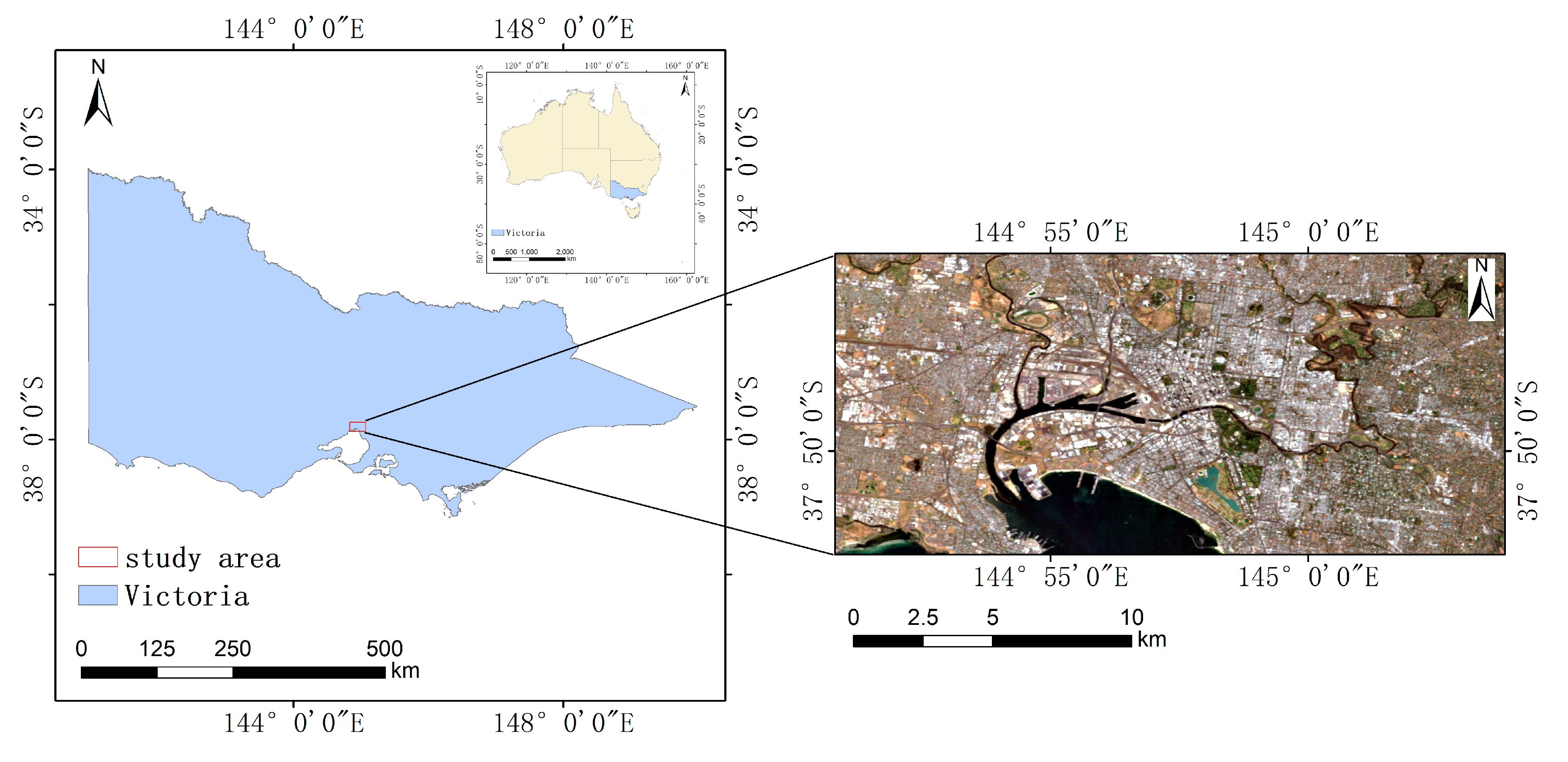
2.1. Study Area
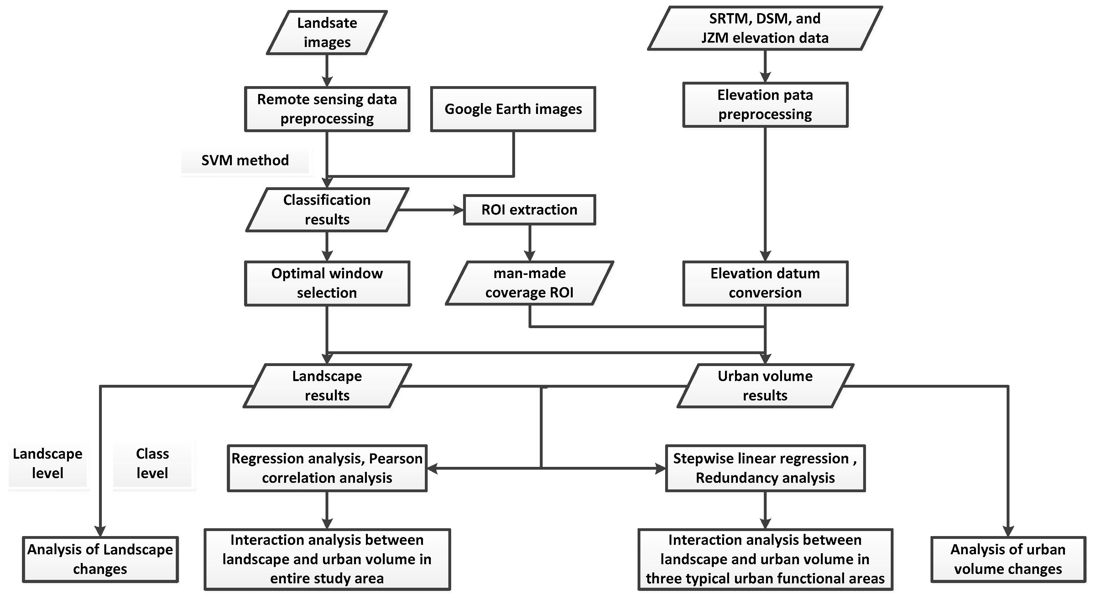
2.2. Workflow
2.3. Remote Sensing Data Processing and Landscape Pattern Calculation
2.4. Elevation Data Processing and Volume Calculation
2.5. Statistical Analysis
3. Results
3.1. The Spatiotemporal Pattern of Landscape and Volume
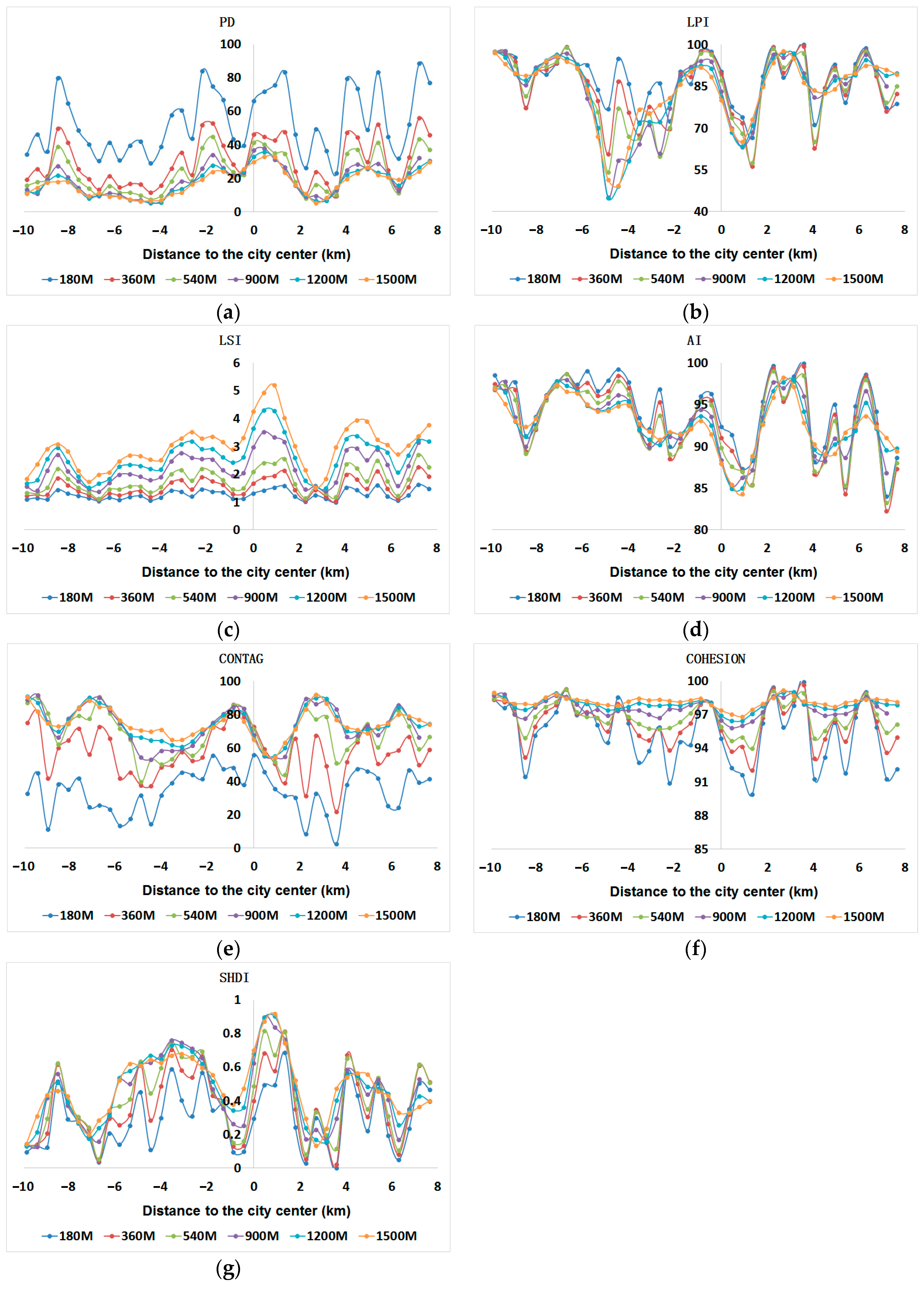
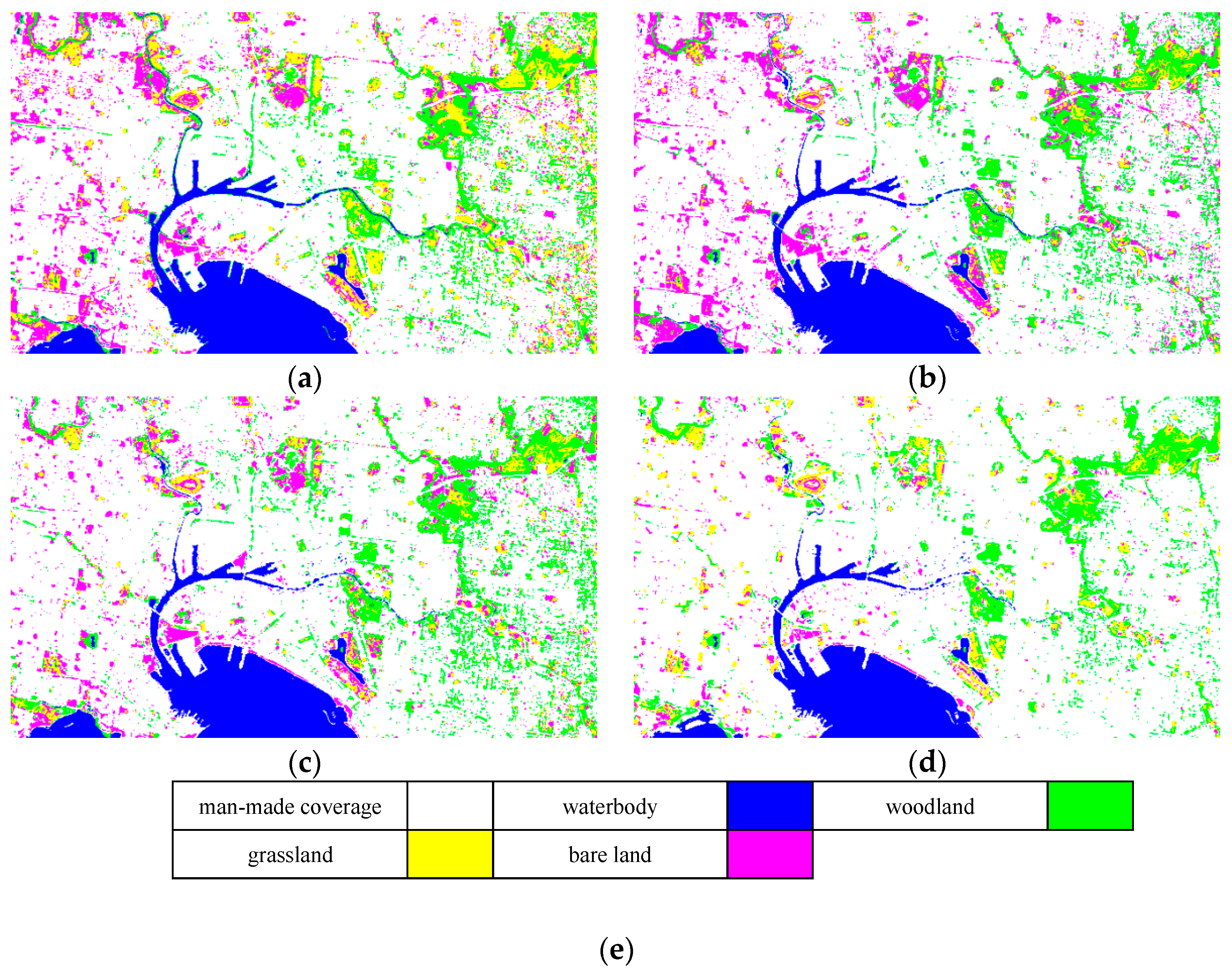
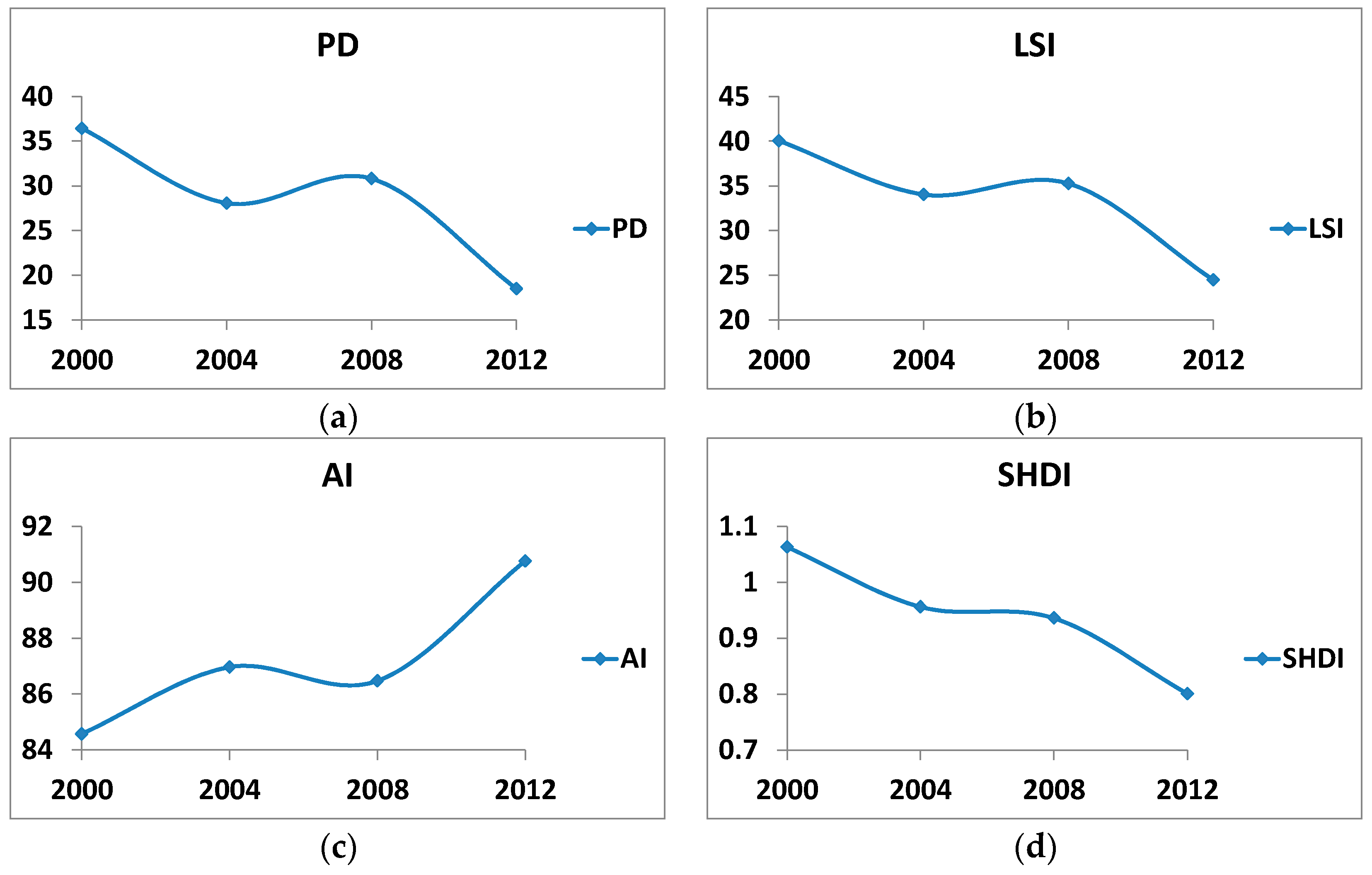
3.1.1. Landscape Pattern Changes
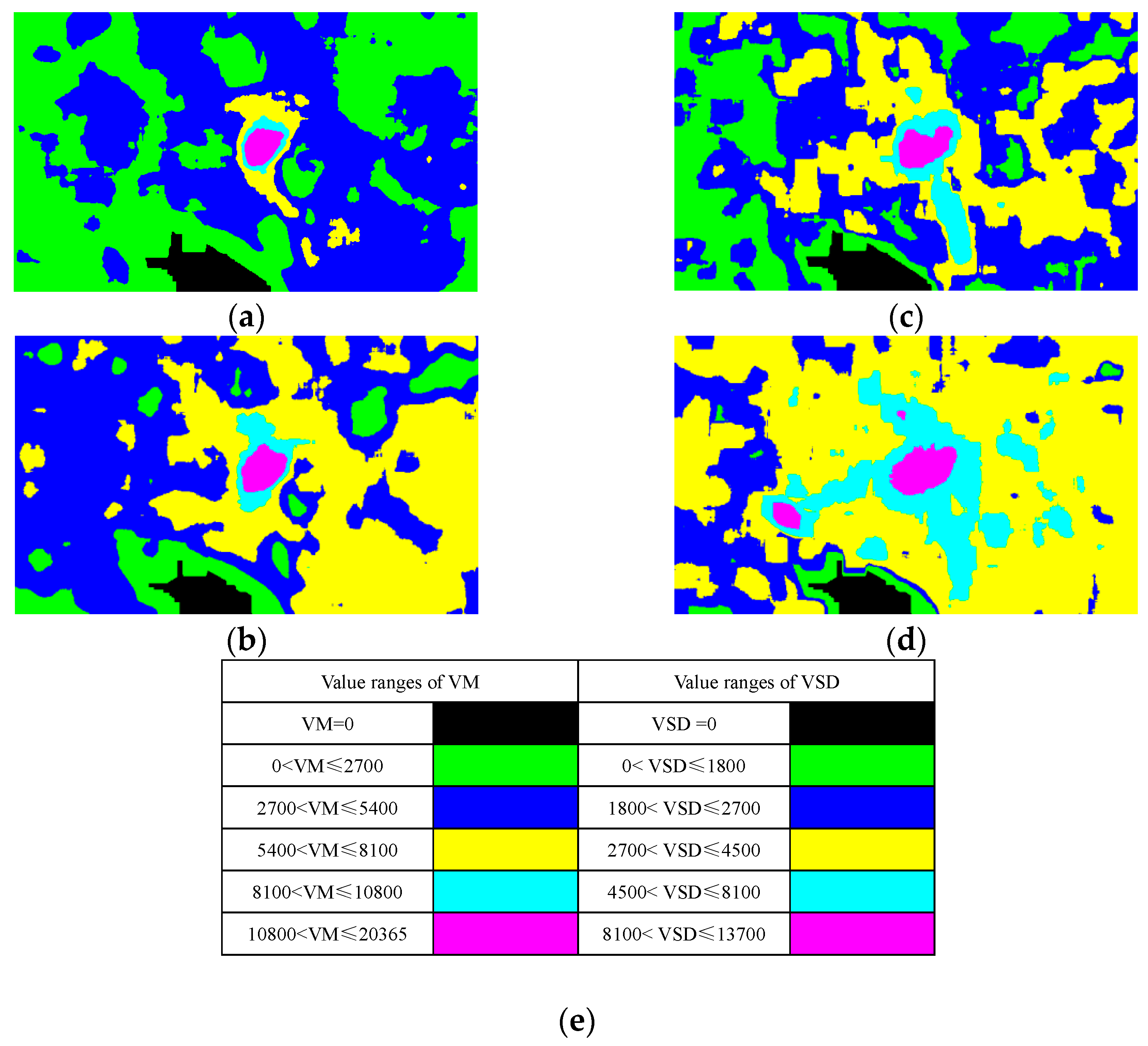
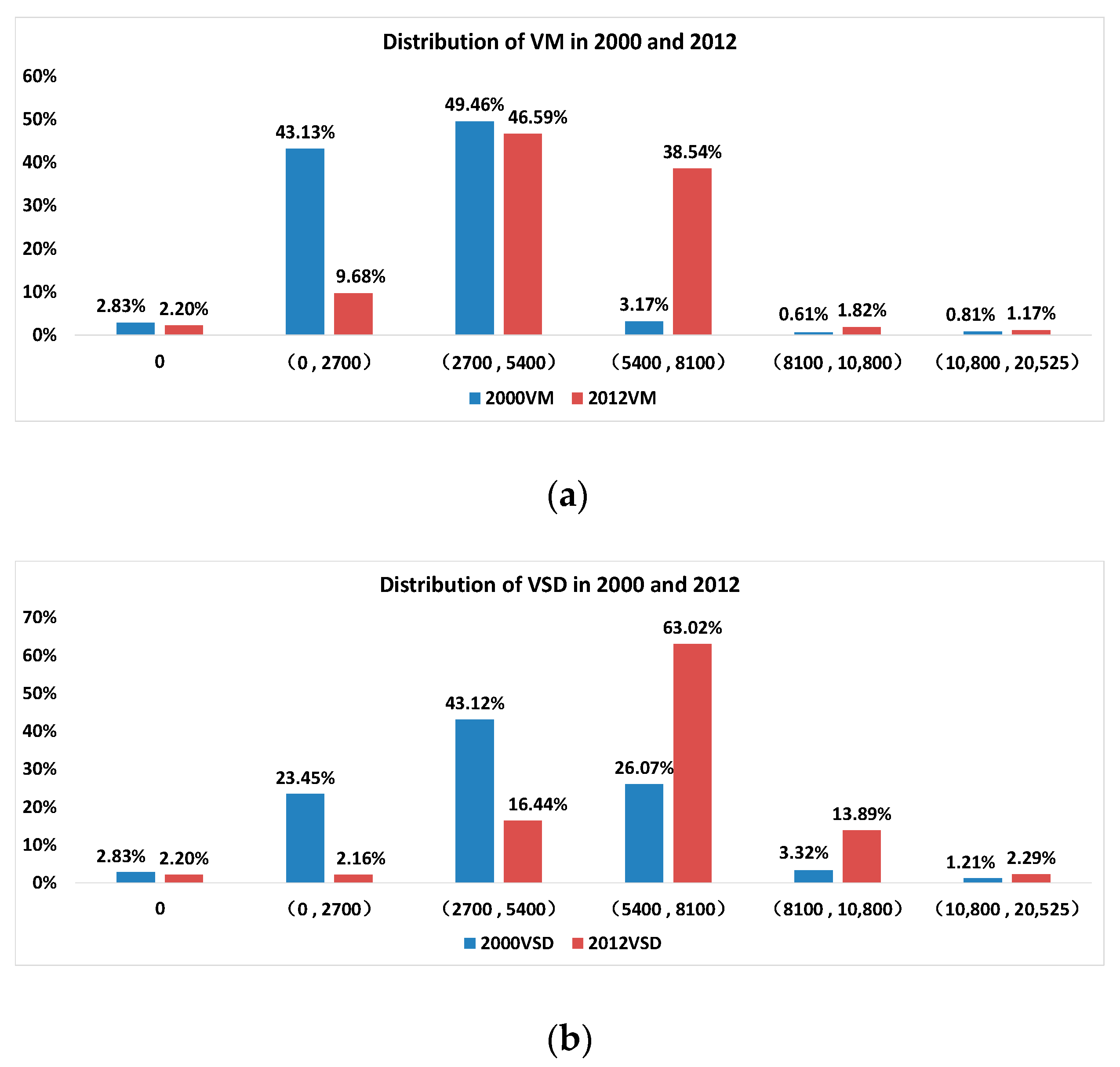
3.1.2. Urban Volume Change
3.2. Correlation and Changes within Different Areas
3.2.1. Entire Study Area
3.2.2. Three Typical Urban Functional Areas
4. Discussion
4.1. Reasons for the Change of Different Dimensions in Melbourne
4.2. Quantitative Analysis and Suggestions
4.2.1. Entire Study Area
4.2.2. Three Typical Urban Functional Areas
5. Conclusions
Author Contributions
Funding
Data Availability Statement
Acknowledgments
Conflicts of Interest
Appendix A

| VM | ||||||||
|---|---|---|---|---|---|---|---|---|
| Year | Landscape Metrics | Regression Equations | Pearson | Landscape Metrics | Regression Equations | Pearson | ||
| 2000 | PD | 0.27 ** | + | PLAND3 | NSc | |||
| 2012 | 0.17 ** | - | NSc | |||||
| 2000 | LPI | 0.13 ** | + | PD3 | 0.15 ** | + | ||
| 2012 | 0.17 ** | + | NSc | |||||
| 2000 | LSI | NSc | LPI3 | NSc | ||||
| 2012 | 0.12 ** | - | NSc | |||||
| 2000 | AI | NSc | LSI3 | 0.14 ** | + | |||
| 2012 | 0.11 ** | + | 0.12 ** | + | ||||
| 2000 | CONTAG | 0.30 ** | + | AI3 | 0.18 ** | + | ||
| 2012 | 0.48 ** | + | 0.16 ** | + | ||||
| 2000 | COHESION | NSc | COHESION3 | 0.17 ** | + | |||
| 2012 | 0.11 ** | + | 0.22 ** | + | ||||
| 2000 | SHDI | 0.25 ** | - | |||||
| 2012 | 0.16 ** | - | ||||||
| 2000 | PLAND1 | 0.88 ** | + | PLAND4 | NSc | |||
| 2012 | 0.92 ** | + | 0.13 ** | - | ||||
| 2000 | PD1 | NSc | PD4 | NSc | ||||
| 2012 | NSc | 0.11 ** | - | |||||
| 2000 | LPI1 | 0.85 ** | + | LPI4 | NSc | |||
| 2012 | 0.91 ** | + | 0.11 ** | - | ||||
| 2000 | LSI1 | 0.27 ** | - | LSI4 | NSc | |||
| 2012 | 0.15 ** | - | 0.11 ** | - | ||||
| 2000 | AI1 | 0.81 ** | + | AI4 | NSc | |||
| 2012 | 0.82 ** | + | 0.13 ** | - | ||||
| 2000 | COHESION1 | 0.87 ** | + | COHESION4 | 0.15 ** | + | ||
| 2012 | 0.88 ** | + | 0.25 ** | - | ||||
| 2000 | PLAND2 | 0.57 ** | - | PLAND5 | 0.15 ** | - | ||
| 2012 | 0.65 ** | - | NSc | |||||
| 2000 | PD2 | 0.24 ** | + | PD5 | NSc | |||
| 2012 | 0.26 ** | + | NSc | - | ||||
| 2000 | LPI2 | 0.58 ** | - | LPI5 | 0.14 ** | - | ||
| 2012 | 0.66 ** | - | NSc | |||||
| 2000 | LSI2 | NSc | LSI5 | 0.11 ** | - | |||
| 2012 | 0.21 ** | + | NSc | - | ||||
| 2000 | AI2 | 0.16 ** | - | AI5 | 0.14 ** | - | ||
| 2012 | 0.23 ** | - | NSc | |||||
| 2000 | COHESION2 | 0.15 ** | - | COHESION5 | 0.18 ** | - | ||
| 2012 | 0.23 ** | - | NSc | |||||
| VSD | ||||||||
|---|---|---|---|---|---|---|---|---|
| Year | Landscape Metrics | Regression Equations | Pearson | Landscape Metrics | Regression Equations | Pearson | ||
| 2000 | PD | 0.39 ** | + | PLAND3 | 0.20 ** | + | ||
| 2012 | 0.33 ** | + | NSc | |||||
| 2000 | LPI | NSc | PD3 | 0.30 ** | + | |||
| 2012 | NSc | NSc | ||||||
| 2000 | LSI | 0.22 ** | + | LPI3 | NSc | |||
| 2012 | 0.16 ** | + | NSc | |||||
| 2000 | AI | 0.13 ** | - | LSI3 | 0.31 ** | + | ||
| 2012 | NSc | 0.15 ** | + | |||||
| 2000 | CONTAG | NSc | AI3 | 0.16 ** | + | |||
| 2012 | 0.14 ** | + | 0.16 ** | + | ||||
| 2000 | COHESION | 0.13 ** | - | COHESION3 | 0.23 ** | + | ||
| 2012 | NSc | 0.18 ** | + | |||||
| 2000 | SHDI | 0.51 ** | + | |||||
| 2012 | 0.29 ** | + | ||||||
| 2000 | PLAND1 | 0.57 ** | + | PLAND4 | NSc | |||
| 2012 | 0.55 ** | + | NSc | |||||
| 2000 | PD1 | 0.22 ** | + | PD4 | NSc | |||
| 2012 | 0.15 ** | + | NSc | |||||
| 2000 | LPI1 | 0.50 ** | + | LPI4 | NSc | |||
| 2012 | 0.51 ** | + | NSc | |||||
| 2000 | LSI1 | 0.46 ** | + | LSI4 | NSc | |||
| 2012 | 0.39 ** | + | NSc | |||||
| 2000 | AI1 | 0.62 ** | + | AI4 | 0.13 ** | + | ||
| 2012 | 0.55 ** | + | NSc | |||||
| 2000 | COHESION1 | 0.70 ** | + | COHESION4 | 0.13 ** | + | ||
| 2012 | 0.63 ** | + | NSc | |||||
| 2000 | PLAND2 | 0.38 ** | - | PLAND5 | NSc | |||
| 2012 | 0.37 ** | - | NSc | |||||
| 2000 | PD2 | 0.29 ** | + | PD5 | NSc | |||
| 2012 | 0.37 ** | + | NSc | |||||
| 2000 | LPI2 | 0.40 ** | - | LPI5 | NSc | |||
| 2012 | 0.40 ** | - | NSc | |||||
| 2000 | LSI2 | 0.11 ** | + | LSI5 | NSc | |||
| 2012 | 0.28 ** | + | NSc | |||||
| 2000 | AI2 | 0.16 ** | + | AI5 | NSc | |||
| 2012 | . | 0.20 ** | + | NSc | ||||
| 2000 | COHESION2 | 0.16 ** | + | COHESION5 | NSc | |||
| 2012 | 0.21 ** | + | NSc | |||||
| 2000 | 2012 | ||||||||||||
|---|---|---|---|---|---|---|---|---|---|---|---|---|---|
| VM | VSD | VM | VSD | ||||||||||
| Landscape Metrics | Standardized Coefficients | Tolerance | VIF | Standardized Coefficients | Tolerance | VIF | Landscape Metrics | Standardized Coefficients | Tolerance | VIF | Standardized Coefficients | Tolerance | VIF |
| LPI3 | −0.390 ** | 0.477 | 2.098 | -- | -- | -- | COHESION2 | -- | -- | -- | 0.573 ** | 0.685 | 1.460 |
| AI3 | 0.156 ** | 0.517 | 1.936 | -- | -- | -- | PLAND3 | −0.454 ** | 0.464 | 2.157 | -- | -- | -- |
| COHESION3 | -- | -- | -- | 0.281 ** | 0.854 | 1.171 | PD3 | 0.281 ** | 0.333 | 3.000 | -- | -- | -- |
| PD4 | -- | -- | -- | −0.303 ** | 0.476 | 2.100 | PD4 | 0.325 ** | 0.624 | 1.603 | −0.447 ** | 0.685 | 1.460 |
| LPI4 | -- | -- | -- | 0.324 ** | 0.669 | 1.494 | R2 | 0.22 | 0.82 | ||||
| COHESION4 | −0.113 ** | 0.411 | 2.433 | -- | -- | -- | |||||||
| PD5 | 0.688 ** | 0.555 | 1.800 | −0.366 ** | 0.554 | 1.805 | |||||||
| LPI5 | −0.206 ** | 0.279 | 3.582 | -- | -- | -- | |||||||
| AI5 | -- | -- | -- | −0.247 ** | 0.736 | 1.359 | |||||||
| COHESION5 | 0.251 ** | 0.308 | 3.244 | -- | -- | -- | |||||||
| R2 | 0.81 | 0.53 | |||||||||||
| 2000 | 2012 | ||||||||||||
|---|---|---|---|---|---|---|---|---|---|---|---|---|---|
| VM | VSD | VM | VSD | ||||||||||
| Landscape Metrics | Standardized Coefficients | Tolerance | VIF | Standardized Coefficients | Tolerance | VIF | Landscape Metrics | Standardized Coefficients | Tolerance | VIF | Standardized Coefficients | Tolerance | VIF |
| PD2 | -- | -- | -- | 0.611 ** | 0.769 | 1.301 | PD2 | -- | -- | -- | 0.491 ** | 0.866 | 1.155 |
| COHESION2 | -- | -- | -- | 0.090 ** | 0.578 | 1.730 | AI3 | −0.319 ** | 0.664 | 1.506 | −0.135 ** | 0.628 | 1.593 |
| PD4 | -- | -- | -- | −0.226 ** | 0.634 | 1.577 | LSI4 | −0.441 ** | 0.604 | 1.657 | −0.278 ** | 0.705 | 1.419 |
| AI4 | −0.437 ** | 1.000 | 1.000 | -- | -- | -- | LSI5 | −0.554 ** | 0.565 | 1.770 | -- | -- | -- |
| LSI5 | -- | -- | -- | −0.163 ** | 0.632 | 1.583 | AI5 | 0.248 ** | 0.530 | 1.888 | -- | -- | -- |
| AI5 | -- | -- | -- | −0.054 ** | 0.805 | 1.242 | R2 | 0.61 | 0.47 | ||||
| R2 | 0.19 | 0.59 | |||||||||||
| 2000 | 2012 | ||||||||||||
|---|---|---|---|---|---|---|---|---|---|---|---|---|---|
| VM | VSD | VM | VSD | ||||||||||
| Landscape Metrics | Standardized Coefficients | Tolerance | VIF | Standardized Coefficients | Tolerance | VIF | Landscape Metrics | Standardized Coefficients | Tolerance | VIF | Standardized Coefficients | Tolerance | VIF |
| PD1 | -- | -- | -- | 0.429 ** | 0.550 | 1.818 | LSI3 | −0.347 ** | 0.646 | 1.548 | -- | -- | -- |
| LPI1 | 0.842 ** | 0.185 | 5.416 | -- | -- | -- | COHESION3 | -- | -- | -- | 0.541 ** | 0.811 | 1.233 |
| PD3 | -- | -- | -- | 0.157 ** | 0.680 | 1.470 | PLAND4 | -- | -- | -- | −0.077 ** | 0.990 | 1.010 |
| COHESION3 | 0.194 ** | 0.337 | 2.965 | -- | -- | -- | AI4 | −0.170 ** | 0.746 | 1.340 | -- | -- | -- |
| PLADN4 | −0.331 ** | 0.210 | 4.769 | -- | -- | -- | LPI5 | -- | -- | -- | 0.530 ** | 0.818 | 1.222 |
| AI4 | −0.094 ** | 0.633 | 1.579 | -- | -- | -- | LSI5 | 0.214 ** | 0.642 | 1.557 | -- | -- | -- |
| COHESION4 | -- | -- | -- | 0.190 ** | 0.695 | 1.438 | R2 | 0.08 | 0.83 | ||||
| LSI5 | 0.218 ** | 0.475 | 2.104 | 0.226 ** | 0.547 | 1.829 | |||||||
| R2 | 0.80 | 0.63 | |||||||||||
References
- Bian, Z.; Wang, S.; Wang, Q.; Yu, M.; Qian, F. Effects of urban sprawl on arthropod communities in peri-urban farmed landscape in Shenbei New District, Shenyang, Liaoning Province, China. Sci. Rep. 2018, 8, 101. [Google Scholar] [CrossRef]
- Schneider, A.; Mertes, C.M. Expansion and growth in Chinese cities, 1978–2010. Environ. Res. Lett. 2014, 9, 024008. [Google Scholar] [CrossRef]
- Li, X.; Liu, X.; Gong, P. Integrating ensemble-urban cellular automata model with an uncertainty map to improve the performance of a single model. Int. J. Geogr. Inf. Sci. 2015, 29, 762–785. [Google Scholar] [CrossRef]
- Effat, H.A.; El Shobaky, M.A. Modeling and Mapping of Urban Sprawl Pattern in Cairo Using Multi-Temporal Landsat Images, and Shannon’s Entropy. Adv. Remote Sens. 2015, 04, 303–318. [Google Scholar] [CrossRef] [Green Version]
- Peng, Y.; Wang, Q.; Wang, H.; Lin, Y.; Song, J.; Cui, T.; Fan, M. Does landscape pattern influence the intensity of drought and flood? Ecol. Indic. 2019, 103, 173–181. [Google Scholar] [CrossRef]
- Seto, K.C.; Guneralp, B.; Hutyra, L.R. Global forecasts of urban expansion to 2030 and direct impacts on biodiversity and carbon pools. Proc. Natl. Acad. Sci. USA 2012, 109, 16083–16088. [Google Scholar] [CrossRef] [PubMed] [Green Version]
- Peng, J.; Ma, J.; Liu, Q.; Liu, Y.; Hu, Y.; Li, Y.; Yue, Y. Spatial-temporal change of land surface temperature across 285 cities in China: An urban-rural contrast perspective. Sci. Total Environ. 2018, 635, 487–497. [Google Scholar] [CrossRef]
- Hua, S.; Jing, H.; Yao, Y.; Guo, Z.; Lerner, D.N.; Andrews, C.B.; Zheng, C. Can groundwater be protected from the pressure of China’s urban growth? Environ. Int. 2020, 143, 105911. [Google Scholar] [CrossRef]
- Yang, G.; Zhao, Y.; Xing, H.; Fu, Y.; Liu, G.; Kang, X.; Mai, X. Understanding the changes in spatial fairness of urban greenery using time-series remote sensing images: A case study of Guangdong-Hong Kong-Macao Greater Bay. Sci. Total Environ. 2020, 715, 136763. [Google Scholar] [CrossRef]
- Shi, L.; Wurm, M.; Huang, X.; Zhong, T.; Leichtle, T.; Taubenböck, H. Urbanization that hides in the dark-Spotting China’s “ghost neighborhoods” from space. Landsc. Urban Plan. 2020, 200, 103822. [Google Scholar] [CrossRef]
- Rimal, B.; Zhang, L.; Keshtkar, H.; Wang, N.; Lin, Y. Monitoring and Modeling of Spatiotemporal Urban Expansion and Land-Use/Land-Cover Change Using Integrated Markov Chain Cellular Automata Model. ISPRS Int. J. Geo-Inf. 2017, 6, 288. [Google Scholar] [CrossRef] [Green Version]
- Peng, J.; Liu, Y.; Wu, J.; Lv, H.; Hu, X. Linking ecosystem services and landscape patterns to assess urban ecosystem health: A case study in Shenzhen City, China. Landsc. Urban Plan. 2015, 143, 56–68. [Google Scholar] [CrossRef]
- Wu, J.; Hobbs, R. Key issues and research priorities in landscape ecology: An idiosyncratic synthesis. Landsc. Ecol. 2002, 17, 355–365. [Google Scholar] [CrossRef]
- Li, X.; Yeh, A.G. Analyzing spatial restructuring of land use patterns in a fast growing region using remote sensing and GIS. Landsc. Urban Plan. 2004, 69, 335–354. [Google Scholar] [CrossRef]
- Yu, X.; Ng, C. An integrated evaluation of landscape change using remote sensing and landscape metrics: A case study of Panyu, Guangzhou. Int. J. Remote Sens. 2006, 27, 1075–1092. [Google Scholar] [CrossRef]
- Weng, Q. Land use change analysis in the Zhujiang Delta of China using satellite remote sensing, GIS and stochastic modelling. J. Environ. Manag. 2002, 64, 273–284. [Google Scholar] [CrossRef] [Green Version]
- Ji, W.; Ma, J.; Twibell, R.W.; Underhill, K. Characterizing urban sprawl using multi-stage remote sensing images and landscape metrics. Comput. Environ. Urban Syst. 2006, 30, 861–879. [Google Scholar] [CrossRef]
- Bosch, M.; Jaligot, R.; Chenal, J. Spatiotemporal patterns of urbanization in three Swiss urban agglomerations: Insights from landscape metrics, growth modes and fractal analysis. Landsc. Ecol. 2020, 35, 879–891. [Google Scholar] [CrossRef]
- Qiu, J.; Wang, X.; Lu, F.; Ouyang, Z.; Zheng, H. The spatial pattern of landscape fragmentation and its relations with urbanization and socio-economic developments: A case study of Beijing. Acta Ecol. Sin. 2012, 32, 2659–2669. [Google Scholar]
- Felt, C.; Fragkias, M.; Larson, D.; Liao, H.; Lohse, K.A.; Lybecker, D. A comparative study of urban fragmentation patterns in small and mid-sized cities of Idaho. Urban Ecosyst. 2018, 21, 805–816. [Google Scholar] [CrossRef]
- Silva, P.; Li, L. Mapping Urban Expansion and Exploring Its Driving Forces in the City of Praia, Cape Verde, from 1969 to 2015. Sustainability 2017, 9, 1434. [Google Scholar] [CrossRef] [Green Version]
- Qin, J.; Fang, C.; Wang, Y.; Li, G.; Wang, S. Evaluation of three-dimensional urban expansion: A case study of Yangzhou City, Jiangsu Province, China. Chin. Geogr. Sci. 2015, 25, 224–236. [Google Scholar] [CrossRef]
- He, S.; Wang, X.; Dong, J.; Wei, B.; Duan, H.; Jiao, J.; Xie, Y. Three-Dimensional Urban Expansion Analysis of Valley-Type Cities: A Case Study of Chengguan District, Lanzhou, China. Sustainability 2019, 11, 5663. [Google Scholar] [CrossRef] [Green Version]
- Zheng, Z.; Zhou, W.; Wang, J.; Hu, X.; Qian, Y. Sixty-Year Changes in Residential Landscapes in Beijing: A Perspective from Both the Horizontal (2D) and Vertical (3D) Dimensions. Remote Sens. 2017, 9, 992. [Google Scholar] [CrossRef] [Green Version]
- Shi, L.; Foody, G.M.; Boyd, D.S.; Girindran, R.; Wang, L.; Du, Y.; Ling, F. Night-time lights are more strongly related to urban building volume than to urban area. Remote Sens. Lett. 2019, 11, 29–36. [Google Scholar] [CrossRef]
- Qiao, W.; Liu, Y.; Wang, Y.; Lu, Y. Analysis on the characteristics of three-dimensional urban space expansion in Nanjing since 2000. Geogr. Res. 2015, 34, 666–676. [Google Scholar]
- van Leeuwen, C.J. Water governance and the quality of water services in the city of Melbourne. Urban Water J. 2017, 14, 247–254. [Google Scholar] [CrossRef]
- Sokolov, S.; Black, K.P. Modelling the time evolution of water-quality parameters in a river: Yarra River, Australia. J. Hydrol. 1996, 178, 311–335. [Google Scholar] [CrossRef]
- Coutts, A.M.; Beringer, J.; Tapper, N.J. Impact of Increasing Urban Density on Local Climate: Spatial and Temporal Variations in the Surface Energy Balance in Melbourne, Australia. J. Appl. Meteorol. Clim. 2007, 46, 477–493. [Google Scholar] [CrossRef]
- Department of Sustainability and Environment. Melbourne 2030: Planning for Sustainable Growth, State of Victoria; Department of Sustainability and Environment: Melbourne, Australia, 2002; p. 192.
- Zhang, H.; Wang, T.; Zhang, Y.; Dai, Y.; Jia, J.; Yu, C.; Li, G.; Lin, Y.; Lin, H.; Cao, Y. Quantifying Short-Term Urban Land Cover Change with Time Series Landsat Data: A Comparison of Four Different Cities. Sensors 2018, 18, 4319. [Google Scholar] [CrossRef] [Green Version]
- Feranec, J.; Jaffrain, G.; Soukup, T.; Hazeu, G. Determining changes and flows in European landscapes 1990–2000 using CORINE land cover data. Appl. Geogr. 2010, 30, 19–35. [Google Scholar] [CrossRef]
- Gong, P.; Wang, J.; Yu, L.; Zhao, Y.; Zhao, Y.; Liang, L.; Niu, Z.; Huang, X.; Fu, H.; Liu, S.; et al. Finer resolution observation and monitoring of global land cover: First mapping results with Landsat TM and ETM+ data. Int. J. Remote Sens. 2012, 34, 2607–2654. [Google Scholar] [CrossRef] [Green Version]
- Xiao, R.; Huang, X.; Yu, W.; Lin, M.; Zhang, Z. Interaction Relationship between Built-Up Land Expansion and Demographic-Social-Economic Urbanization in Shanghai-Hangzhou Bay Metropolitan Region of Eastern China. Photogramm. Eng. Remote Sens. 2019, 85, 231–240. [Google Scholar] [CrossRef]
- Li, X.; Gong, P.; Liang, L. A 30-year (1984–2013) record of annual urban dynamics of Beijing City derived from Landsat data. Remote Sens. Environ. 2015, 166, 78–90. [Google Scholar] [CrossRef]
- Gong, W.; Fang, S.; Yang, G.; Ge, M. Using a Hidden Markov Model for Improving the Spatial-Temporal Consistency of Time Series Land Cover Classification. ISPRS Int. J. Geo-Inf. 2017, 6, 292. [Google Scholar] [CrossRef] [Green Version]
- Hulshoff, R.M. Landscape indices describing a Dutch landscape. Landsc. Ecol. 1995, 10, 101–111. [Google Scholar] [CrossRef]
- Peng, J.; Wang, Y.; Zhang, Y.; Wu, J.; Li, W.; Li, Y. Evaluating the effectiveness of landscape metrics in quantifying spatial patterns. Ecol. Indic. 2010, 10, 217–223. [Google Scholar] [CrossRef]
- Griffiths, G.H.; Lee, J. Landscape pattern and species richness; regional scale analysis from remote sensing. Int. J. Remote Sens. 2000, 21, 2685–2704. [Google Scholar] [CrossRef]
- Junxiang, L.; Yujie, W.; Xiaohong, S.; Yongchang, S. Landscape pattern analysis along an urban-rural gradient in the Shanghai metropolitan region. Acta Ecol. Sin. 2004, 24, 1973–1980. [Google Scholar]
- Saura, S. Effects of remote sensor spatial resolution and data aggregation on selected fragmentation indices. Landsc. Ecol. 2004, 19, 197–209. [Google Scholar] [CrossRef]
- Wu, Q.; Guo, F.; Li, H.; Kang, J. Measuring landscape pattern in three dimensional space. Landsc. Urban Plan. 2017, 167, 49–59. [Google Scholar] [CrossRef]
- Zhou, W.; Cao, F.; Wang, G. Effects of Spatial Pattern of Forest Vegetation on Urban Cooling in a Compact Megacity. Forests 2019, 10, 282. [Google Scholar] [CrossRef] [Green Version]
- He, H.S.; DeZonia, B.E.; Mladenoff, D.J. An aggregation index (AI) to quantify spatial patterns of landscapes. Landsc. Ecol. 2000, 15, 591–601. [Google Scholar] [CrossRef]
- Chuncheng, Z.; Youshui, Z.; Huanhuan, H. Impacts of Impervious Surface Area and Landscape Metrics on Urban Heat Environment in Fuzhou City, China. J. Geo-Inf. Sci. 2014, 16, 490–498. [Google Scholar]
- Hagen-Zanker, A. A computational framework for generalized moving windows and its application to landscape pattern analysis. Int. J. Appl. Earth Obs. 2016, 44, 205–216. [Google Scholar] [CrossRef] [Green Version]
- Park, Y.; Guldmann, J. Measuring continuous landscape patterns with Gray-Level Co-Occurrence Matrix (GLCM) indices: An alternative to patch metrics? Ecol. Indic. 2020, 109, 105802. [Google Scholar] [CrossRef]
- Chen, Y.; Li, X.; Liu, X.; Ai, B. Modeling urban land-use dynamics in a fast developing city using the modified logistic cellular automaton with a patch-based simulation strategy. Int. J. Geogr. Inf. Sci. 2014, 28, 234–255. [Google Scholar] [CrossRef]
- Fan, C.; Myint, S. A comparison of spatial autocorrelation indices and landscape metrics in measuring urban landscape fragmentation. Landsc. Urban Plan. 2014, 121, 117–128. [Google Scholar] [CrossRef]
- Yang, Q.; Li, J.; Gan, X.; Zhang, J.; Yang, F.; Qian, Y. Comparison of landscape patterns between metropolises and small-sized cities: A gradient analysis with changing grain size in Shanghai and Zhangjiagang, China. Int. J. Remote Sens. 2012, 33, 1446–1464. [Google Scholar] [CrossRef]
- Luck, M.; Wu, J. A gradient analysis of urban landscape pattern: A case study from the Phoenix metropolitan region, Arizona, USA. Landsc. Ecol. 2002, 17, 327–339. [Google Scholar] [CrossRef]
- Zhang, J.; Li, S.; Dong, R.; Jiang, C. Physical evolution of the Three Gorges Reservoir using advanced SVM on Landsat images and SRTM DEM data. Environ. Sci. Pollut. Res. 2018, 25, 14911–14918. [Google Scholar] [CrossRef] [PubMed]
- Priestnall, G.; Jaafar, J.; Duncan, A. Extracting urban features from LiDAR digital surface models. Comput. Environ. Urban Syst. 2000, 24, 65–78. [Google Scholar] [CrossRef]
- Ali, Z.; Nasir, S.; Iqbal, I.A.; Shahzad, A. Accuracy Assessment of Digital Elevation Model Generated from Pleiades Tri stereo-pair. In Proceedings of the International Conference on Recent Advances in Space Technologies, Istanbul, Turkey, 16–19 June 2015. [Google Scholar]
- Yao, X.; Sun, M.; Gong, P.; Liu, B.; Li, X.; An, L.; Yan, L. Overflow probability of the Salt Lake in Hoh Xil Region. J. Geogr. Sci. 2018, 28, 647–655. [Google Scholar] [CrossRef] [Green Version]
- Islam, M.A.; Thenkabail, P.S.; Kulawardhana, R.W.; Alankara, R.; Gunasinghe, S.; Edussriya, C.; Gunawardana, A. Semi-automated methods for mapping wetlands using Landsat ETM+ and SRTM data. Int. J. Remote Sens. 2008, 29, 7077–7106. [Google Scholar] [CrossRef]
- Wu, Q.; Song, C.; Liu, K.; Ke, L. Integration of TanDEM-X and SRTM DEMs and Spectral Imagery to Improve the Large-Scale Detection of Opencast Mining Areas. Remote Sens. 2020, 12, 1451. [Google Scholar] [CrossRef]
- Zhang, Q.; Yang, Q.; Cheng, J.; Wang, C. Characteristics of 3″ SRTM Errors in China. Geomat. Inf. Sci. Wuhan Univ. 2018, 43, 684–690. [Google Scholar]
- Nelson, A.D.; Reuter, H.I.; Gessler, P.; Hengl, T.; Reuter, H.I. Dem Production methods and sources. Dev. Soil Sci. 2009, 33, 65–85. [Google Scholar]
- Kellndorfer, J.; Walker, W.; Pierce, L.; Dobson, C.; Fites, J.A.; Hunsaker, C.; Vona, J.; Clutter, M. Vegetation height estimation from Shuttle Radar Topography Mission and National Elevation Datasets. Remote Sens. Environ. 2004, 93, 339–358. [Google Scholar] [CrossRef]
- Guo, J.; Kong, X. Foundation of Geodesy; Wuhan University Press: Wuhan, China, 2005. [Google Scholar]
- Kwon, J.H.; Bae, T.; Choi, Y.; Lee, D.; Lee, Y. Geodetic datum transformation to the global geocentric datum for seas and islands around Korea. Geosci. J. 2005, 9, 353–361. [Google Scholar] [CrossRef]
- Li, Y.C.; Sideris, M.G.; Schwarz, K. A numerical investigation on height anomaly prediction in mountainous areas. Bull. Géodésique 1995, 69, 143–156. [Google Scholar] [CrossRef]
- Zhang, F.; Wang, J.; Luo, H. The Comparative and Analysis of Seven-parameter Coordinate Conversion Model. Geomat. Spat. Inf. Technol. 2016, 39, 48–51. [Google Scholar]
- Fu, F.; Liu, Z.; Huang, Q. Three-dimensional urban landscape pattern changes: A case study in the Central Business District of Futian, Shenzhen. Acta Ecol. Sin. 2019, 39, 4299–4308. [Google Scholar]
- Zhao, Y.; Ovando-Montejo, G.A.; Frazier, A.E.; Mathews, A.J.; Flynn, K.C.; Ellis, E.A. Estimating work and home population using lidar-derived building volumes. Int. J. Remote Sens. 2017, 38, 1180–1196. [Google Scholar] [CrossRef]
- Liu, M.; Hu, Y.; Li, C. Landscape metrics for three-dimensional urban building pattern recognition. Appl. Geogr. 2017, 87, 66–72. [Google Scholar] [CrossRef]
- Qu, B.; Ling, J.; Ma, J. A study on the quantitative description and evaluation method of street spatial form in the city business district. New Archit. 2019, 06, 9–14. [Google Scholar]
- Yang, J.; Shi, Y. Approaches and Methods of Urban Vertical Control in Overall Urban Design. Urban Plan. Forum. 2015, 06, 90–98. [Google Scholar]
- Yang, J. Urban Central District Planning Theories and Methods; Southeast University Press: Nanjing, China, 2013. [Google Scholar]
- Li, Z.; You, H.; Wang, Z. Multi-scale effects of urban landscape pattern on plant diversity in Xuzhou City, Jiangsu Province, China. Chin. J. Appl. Ecol. 2018, 29, 1813–1821. [Google Scholar]
- Jingwei, H.; Yiying, Z.; Chengming, T.; Dianguang, X.; Yingmei, L. Effects of Regional Landscape Pattern on the Epidemic of Poplar Rust Disease: A Case Study of Populus alba in Yanqing, Beijing. Sci. Silvae Sin. 2020, 56, 99–108. [Google Scholar]
- Duan, M.; Liu, Y.; Yu, Z.; Li, L.; Wang, C.; Axmacher, J.C. Environmental factors acting at multiple scales determine assemblages of insects and plants in agricultural mountain landscapes of northern China. Agric. Ecosyst. Environ. 2016, 224, 86–94. [Google Scholar] [CrossRef]
- Song, Y.; Song, X.; Shao, G.; Hu, T. Effects of Land Use on Stream Water Quality in the Rapidly Urbanized Areas: A Multiscale Analysis. Water-Sui. 2020, 12, 1123. [Google Scholar] [CrossRef] [Green Version]
- Djoudi, E.A.; Plantegenest, M.; Aviron, S.; Pétillon, J. Local vs. landscape characteristics differentially shape emerging and circulating assemblages of carabid beetles in agroecosystems. Agric. Ecosyst. Environ. 2019, 270–271, 149–158. [Google Scholar] [CrossRef]
- Zhang, J.; Li, S.; Jiang, C. Effects of land use on water quality in a River Basin (Daning) of the Three Gorges Reservoir Area, China: Watershed versus riparian zone. Ecol. Indic. 2020, 113, 106226. [Google Scholar] [CrossRef]
- Stevens, Q.; Hao, C.; Zhang, S.; Xu, C.; Tie, J. The Design of Urban Waterfronts—A Critique of Two Australian “Southbanks” (Sequel). J. Qingdao Technol. Univ. 2008, 77, 173–203. [Google Scholar]
- Ye, M. Cases and Studies on the Suburban Development Policies of Developed Countries; China Architecture & Building Press: Beijing, China, 2010. [Google Scholar]
- Wu, W.; Zhao, S.; Zhu, C.; Jiang, J. A comparative study of urban expansion in Beijing, Tianjin and Shijiazhuang over the past three decades. Landsc. Urban Plan. 2015, 134, 93–106. [Google Scholar] [CrossRef]
- Li, G.; Sun, S.; Fang, C. The varying driving forces of urban expansion in China: Insights from a spatial-temporal analysis. Landsc. Urban Plan. 2018, 174, 63–77. [Google Scholar] [CrossRef]
- Chien, S. Local farmland loss and preservation in China: A perspective of quota territorialization. Land Use Policy 2015, 49, 65–74. [Google Scholar] [CrossRef]
- Shukla, A.; Jain, K. Critical analysis of spatial-temporal morphological characteristic of urban landscape. Arab. J. Geosci. 2019, 12, 112. [Google Scholar] [CrossRef]
- Anim, A.K.; Thompson, K.; Duodu, G.O.; Tscharke, B.; Birch, G.; Goonetilleke, A.; Ayoko, G.A.; Mueller, J.F. Pharmaceuticals, personal care products, food additive and pesticides in surface waters from three Australian east coast estuaries (Sydney, Yarra and Brisbane). Mar. Pollut. Bull. 2020, 153, 111014. [Google Scholar] [CrossRef]
- Bonan, G.B. The microclimates of a suburban Colorado (USA) landscape and implications for planning and design. Landsc. Urban Plan. 2000, 49, 97–114. [Google Scholar] [CrossRef]
- Mehta, V. Walkable streets: Pedestrian behavior, perceptions and attitudes. J. Urban. Int. Res. Placemaking Urban Sustain. 2008, 1, 217–245. [Google Scholar] [CrossRef]
- de Bell, S.; White, M.; Griffiths, A.; Darlow, A.; Taylor, T.; Wheeler, B.; Lovell, R. Spending time in the garden is positively associated with health and wellbeing: Results from a national survey in England. Landsc. Urban Plan. 2020, 200, 103836. [Google Scholar] [CrossRef]
- Marshall, A.J.; Grose, M.J.; Williams, N.S.G. From little things: More than a third of public green space is road verge. Urban For. Urban Green. 2019, 44, 126423. [Google Scholar] [CrossRef]
- Bratman, G.N.; Hamilton, J.P.; Daily, G.C. The impacts of nature experience on human cognitive function and mental health. Ann. N. Y. Acad. Sci. 2012, 1249, 118–136. [Google Scholar] [CrossRef] [PubMed]
- Coutts, A.M.; Beringer, J.; Tapper, N.J. Investigating the climatic impact of urban planning strategies through the use of regional climate modelling: A case study for Melbourne, Australia. Int. J. Clim. 2008, 28, 1943–1957. [Google Scholar] [CrossRef]


| Land Use Types | No. | Feature Types Included in Melbourne | Corresponding Types in CORINE Land-Cover Nomenclature |
|---|---|---|---|
| Manmade coverage | 1 | Residential construction, public facilities, transportation facilities, and other construction lands, etc. | Artificial surfaces |
| Waterbody | 2 | Ocean, urban rivers, ponds, etc. | Water bodies |
| Woodland | 3 | Street trees and natural reserves, etc. | Forest |
| Grassland | 4 | Gardens, football fields, etc. | No |
| Bare land | 5 | The land where the surface is soil and is not covered by vegetation | Open spaces with little or no vegetation |
| Aspects | Landscape Metrics | Application Levels | Description |
|---|---|---|---|
| Fragmentation | Percentage of Landscape (PLAND) | Class | PLAND is the proportion of the area of the corresponding patch type in the total landscape area. In other words, PLAND is the proportional abundance of each patch type in the landscape, which provides basic information on the land use gradient [39]. |
| Patch Density (PD) | Class/Landscape | PD is the number of patches per unit area. Higher PD values indicate the increased extent of subdivision or fragmentation of the corresponding patch type [40]. | |
| Largest Patch Index (LPI) | Class/Landscape | LPI is the percent of the total landscape area occupied by the largest size patch of the class of interest. The larger the LPI, the greater the impact of the largest patch on the whole landscape, and the higher the dominance of this type of patch [41]. | |
| Complexity | Landscape Shape Index (LSI) | Class/Landscape | LSI is calculated by the square amended total patch edge length divided by the total landscape area. LSI describes the complexity of the patch shape and the shape characteristics and possible evolutionary trends of the landscape spatial structure [42]. It is the most effective measure of overall shape complexity [43]. |
| Aggregation | Aggregation Index (AI) | Class/Landscape | AI is the level of aggregation of spatial patterns. It means the non-randomness or aggregation degree of different patch types in the landscape [44]. |
| Contagion Index (CONTAG) | Landscape | CONTAG indicates the degree of reunion or extension of different patch types in the landscape. The probability of adjacent patches belonged to a class is calculated by the number of patches [42]. | |
| Patch Cohesion Index (COHESION) | Class/Landscape | COHESION reflects the physical connectedness of the corresponding patch type and the continuity characteristics of each type. The larger the value, the stronger the continuity [45]. | |
| Diversity | Shannon’s Diversity Index (SHDI) | Landscape | SHDI is based on Shannon’s information-theoretic concept of entropy and is a measure of the degree of homogeneity and complexity of landscape types. The higher the SHDI is, the more abundant the land types are and the more uncertain the information content is. Diversity in landscape pattern is closely related to species diversity in ecology [46]. |
| 2000 | Manmade Coverage | Waterbody | Woodland | Grassland | Bare Land | Total Area in 2000 | |
|---|---|---|---|---|---|---|---|
| 2012 | |||||||
| manmade coverage | 152.17 | 1.38 | 8.44 | 5.18 | 11.31 | 178.49 | |
| waterbody | 0.17 | 17.01 | 0.11 | 0.01 | 0.04 | 17.35 | |
| woodland | 1.20 | 0.10 | 8.91 | 4.51 | 1.44 | 16.16 | |
| grassland | 0.46 | 0.00 | 0.09 | 7.09 | 2.78 | 10.42 | |
| bare land | 1.45 | 0.01 | 0.03 | 0.82 | 2.77 | 5.09 | |
| total area in 2012 | 155.45 | 18.51 | 17.59 | 17.61 | 18.35 | 227.50 | |
| Area change | 23.03 | −1.16 | −1.43 | −7.19 | −13.25 | ||
| Land Use Types | Years | PLAND | PD | LPI | LSI | AI | COHESION |
|---|---|---|---|---|---|---|---|
| Manmade Coverage | 2000 | 68.33 | 1.95 | 62.52 | 35.04 | 91.78 | 99.90 |
| 2004 | 72.16 | 1.42 | 70.05 | 31.14 | 92.92 | 99.93 | |
| 2008 | 73.46 | 1.79 | 72.55 | 32.74 | 92.61 | 99.95 | |
| 2012 | 78.45 | 1.16 | 76.64 | 22.52 | 95.15 | 99.95 | |
| Waterbody | 2000 | 8.13 | 0.49 | 6.99 | 7.74 | 95.27 | 98.81 |
| 2004 | 8.14 | 0.46 | 6.94 | 7.99 | 95.09 | 98.80 | |
| 2008 | 7.93 | 0.57 | 6.14 | 7.94 | 95.05 | 98.20 | |
| 2012 | 7.62 | 0.69 | 6.07 | 7.86 | 95.01 | 98.16 | |
| Woodland | 2000 | 7.73 | 11.84 | 2.02 | 61.91 | 56.05 | 92.43 |
| 2004 | 7.91 | 9.69 | 1.13 | 54.16 | 62.10 | 91.81 | |
| 2008 | 8.76 | 11.84 | 1.03 | 62.06 | 58.65 | 89.95 | |
| 2012 | 7.10 | 7.89 | 1.30 | 47.63 | 64.93 | 92.28 | |
| Grassland | 2000 | 7.74 | 9.29 | 0.36 | 50.05 | 64.64 | 84.50 |
| 2004 | 2.72 | 3.13 | 0.12 | 31.19 | 63.15 | 84.24 | |
| 2008 | 4.03 | 7.44 | 0.28 | 44.77 | 56.19 | 81.44 | |
| 2012 | 4.58 | 3.85 | 0.15 | 35.23 | 67.76 | 85.47 | |
| Bare Land | 2000 | 8.06 | 12.87 | 0.28 | 58.76 | 59.20 | 83.06 |
| 2004 | 9.07 | 13.36 | 0.55 | 59.43 | 61.13 | 85.02 | |
| 2008 | 5.82 | 9.17 | 0.18 | 48.86 | 60.12 | 79.72 | |
| 2012 | 2.24 | 4.90 | 0.10 | 36.81 | 51.60 | 71.43 |
| 2000 | 2012 | Volume Change | Change Rate | |
|---|---|---|---|---|
| VM | 2942.28 | 4861.72 | 1919.44 | 5.44% |
| VSD | 2474.99 | 3648.57 | 1173.58 | 3.95% |
Publisher’s Note: MDPI stays neutral with regard to jurisdictional claims in published maps and institutional affiliations. |
© 2021 by the authors. Licensee MDPI, Basel, Switzerland. This article is an open access article distributed under the terms and conditions of the Creative Commons Attribution (CC BY) license (http://creativecommons.org/licenses/by/4.0/).
Share and Cite
Ge, M.; Fang, S.; Gong, Y.; Tao, P.; Yang, G.; Gong, W. Understanding the Correlation between Landscape Pattern and Vertical Urban Volume by Time-Series Remote Sensing Data: A Case Study of Melbourne. ISPRS Int. J. Geo-Inf. 2021, 10, 14. https://doi.org/10.3390/ijgi10010014
Ge M, Fang S, Gong Y, Tao P, Yang G, Gong W. Understanding the Correlation between Landscape Pattern and Vertical Urban Volume by Time-Series Remote Sensing Data: A Case Study of Melbourne. ISPRS International Journal of Geo-Information. 2021; 10(1):14. https://doi.org/10.3390/ijgi10010014
Chicago/Turabian StyleGe, Mengyu, Shenghui Fang, Yan Gong, Pengjie Tao, Guang Yang, and Wenbing Gong. 2021. "Understanding the Correlation between Landscape Pattern and Vertical Urban Volume by Time-Series Remote Sensing Data: A Case Study of Melbourne" ISPRS International Journal of Geo-Information 10, no. 1: 14. https://doi.org/10.3390/ijgi10010014