Simulation of Bay-Shaped Shorelines after the Construction of Large-Scale Structures by Using a Parabolic Bay Shape Equation

1
Department of Civil Architectural Engineering, Sungkyunkwan University, Suwon 16419, Korea
2
Research Institute of Industrial Technology, Pusan National University, Busan 46241, Korea
3
Graduate School of Water Resources, Sungkyunkwan University, Suwon 16419, Korea
*
Author to whom correspondence should be addressed.
J. Mar. Sci. Eng. 2021, 9(1), 43; https://doi.org/10.3390/jmse9010043
Submission received: 29 November 2020
/
Revised: 26 December 2020
/
Accepted: 30 December 2020
/
Published: 4 January 2021
(This article belongs to the Section Coastal Engineering)
Abstract
:Among the various causes of coastal erosion, the installation of offshore breakwaters is considered the main cause that influences the most serious changes in shorelines. However, without a proper means for predicting such terrain changes, countries and regions continue to suffer from the aftermath of development projects on coastal land. It has been confirmed that the parabolic bay shape equation (PBSE) can accurately predict shoreline changes under the wave climate diffracted as a result of such development projects. This study developed a shoreline change model that has enhanced the previous shoreline change models by applying PBSE to shoreline changes into bay-shaped features. As an analytical comparison with the second term of the GENESIS model, which is an existing and well-known shoreline change model, a similar beach erosion width was obtained for a small beach slope. However, as the beach slope became larger, the result became smaller than that of the GENESIS model. The validity of the model was verified by applying it to satellite images that demonstrated the occurrence of shoreline changes caused by breakwaters for seaports on the eastern coast of Korea; Wonpyeong beach, Yeongrang beach, and Wolcheon beach. As a result, each studied site converged on the static equilibrium planform within several years. Simultaneously, the model enabled the coastal management of the arrangement of seaports to evaluate how the construction of structures causes serious shoreline changes by creating changes to wavefields.
1. Introduction
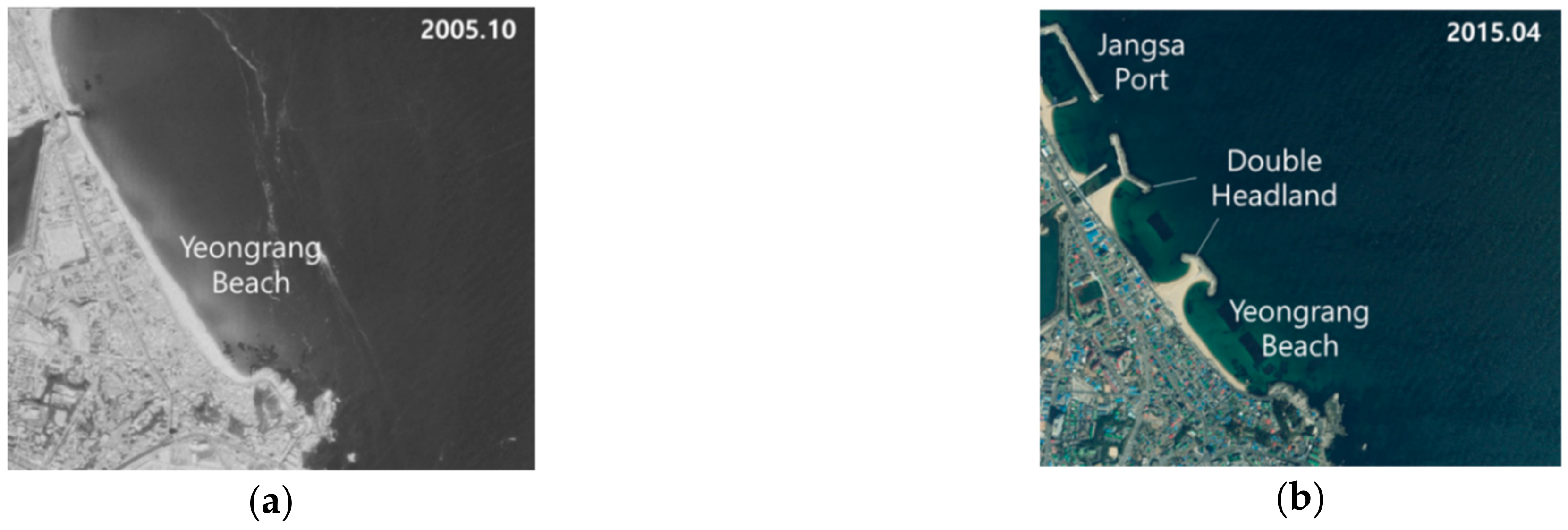
Shores have long played an important part in economic activities and residential lives. Nowadays, shores are gaining more importance, as many people visit coastal resorts every year. However, seaport facilities built on shores trigger changes in wavefields and sediment mobility, thus causing serious erosion in several areas. Accordingly, increasing numbers of shores are carrying out massive sand replenishment or building coastal structures designed to reduce erosion, such as breakwaters or groins. Paradoxically, offshore structures that were built in inappropriate locations resulted in more serious erosion [1]. For example, the loss of sand from the central part of the shore was caused by the double headland method applied to the Yeongrang beach in Sokcho, Gangwon-do, South Korea. A submerged breakwater was built at the center to prevent the problem, but the structure failed to function properly.
Waves changed by structures cause longshore sediment transport to bring about shoreline changes, eventually causing coastal erosion. Many studies have been conducted to elucidate longshore sediment transport and identify theoretical formulas [2,3,4,5,6,7]. Wellen et al. [8] assessed previous longshore sediment formulas for beaches with varying sand grain sizes. However, as the shoreline changes behind the coastal structures built around offshore areas occur because of complex causes, longshore sediment alone is not sufficient as a proper assessment of shoreline changes. For example, breakwaters influence shoreline changes due to factors such as the type of structure, distance from the shore, and waves [9]. Innumerable laboratory experiments [10,11,12,13] could not explain the complex physical phenomena involved in shoreline changes. Therefore, prediction of shoreline changes caused by offshore structures can only rely on empirical research.
The static equilibrium planform (SEP) on shores keeps the shorelines in certain forms by achieving equilibrium in sand mobility [14,15,16]. Much empirical research has been conducted to predict SEP [17,18,19]. Among them, the parabolic bay shape equation (PBSE) proposed by Hsu and Evans [18] has been recognized for its effectiveness and is widely used for coastal management worldwide [20,21,22,23,24,25,26,27,28,29]. Additionally, Lim et al. [30] proved PBSE, in comparison with the longshore sediment transport formula of Coastal Engineering Research Center [5], using wave data on the eastern coast of Korea.
There has been much research carried out on shoreline changes caused by seaports and coastal structures. Pelnard-Considère [31] proposed a governing equation that determines the location of the shoreline according to the difference in longshore sediment transports, which flows along the shore between the berm and closure depth. The equation was obtained under the assumption that the sediments move parallel to the height of the active profile without altering the beach shape but advances or retreats evenly. In reality, longshore sediment transport is superior to cross-shore sediment transport, as a cause that governs shoreline changes in long-term view of point. Bakker [32] presented a two-line model that reflected not only longshore sediment, but also cross-shore sediment. Hulsbergen et al. [33] proved the effectiveness of the model for long, linear coasts through a laboratory experiment.
The one-line shoreline change model presented by Pelnard-Considère [31] could simulate the temporal changes to shorelines caused by the construction of groins on beaches. This model proves its applicability to various situations by applying longshore diffusivity [34,35,36]. The original version did not include the effect of wave diffraction due to a large-scale breakwater or a detached breakwater. Consequently, numerical [37,38,39] and mathematical [40] approaches based on empirical formulas have been followed for the application of the shoreline change model under the circumstance of wave diffraction caused by coastal structures (such as breakwaters or detached breakwaters).
The GENESIS model was developed by Hanson and Kraus [37], including the second term, introduced by Ozasa and Brampton [41], accounting for the longshore sediment transport rate caused by the longshore variation in breaking wave height. This model is often used for engineering consultation with linkage of accurate wave deformation models. Recently, Boussinesq equations and depth-averaged forms of the suspended sediment concentration equation were employed to simulate the coastal sediment transport and shoreline evolution in the presence of coastal structures [42,43].
This study presents a methodology that can be used to remedy the shortcomings of the existing shoreline change models. The present methodology focuses on two aspects as follows. (1) To improve Pelnard-Considère’s shoreline change model [31] to guarantee convergence to a SEP based on PBSE [18]. (2) To simulate depth contour changes. The model assumes that SEP can be applied not only to shorelines, but also to depth contours. Lastly, the model was verified by applying it to the beaches seriously eroded after the construction of large-scale port or harbor structures.
2. One-Line Shoreline Change Model Using Longshore Sediment Transport Equation
Longshore sediment moves along the shoreline when a wave is obliquely incident on the shoreline. Komar and Inman [4] performed an on-site test on longshore energy flux, , and longshore sediment transport, , and presented a formula as displayed in Equation (1).
Here, ,, and indicate the longshore transport rate (immersed weight), sediment density, and seawater density, respectively. indicates sediment porosity, with a value between 0.3 and 0.4. denotes a longshore sediment coefficient that can have wide-ranging values between 0.04 and 1.1, depending on the sediment transport; however, 0.77, as suggested by Komar and Inman [4], is frequently applied. The longshore energy flux, , is defined in Equation (2).
Here, is the wave energy, is the group velocity, and is the wave angle at the breaking point. In the present study, the structure-induced wave diffraction is taken into account by using a PBSE. The CERC [5] suggested Equation (3) by expressing Equation (1) as a formula for wave energy and group velocity against breaking wave height.
Here, is the breaking wave height. is a coefficient related to specific weight, the porosity of sediment that is unrelated to wave conditions and is as displayed in Equation (4). Applying longshore sediment coefficient , wave breaking coefficient , specific gravity , and porosity that are applied to typical shoreline sand yields generates a value of approximately 0.167.
The present shoreline change model is based on the theory of Pelnard-Considère [31] derived based on the law of conservation of sedimentary matter. The gradient of the longshore sediment transport only causes shoreline advances and retreats, ignoring the cross-shore sediment transport.
Here, refers to the closure depth, refers to the height of the berm, and refers to the sediment transport within a specific period, which can be estimated by applying the longshore sediment transport as displayed in Equation (3). Further, refers to the location of the cross-shore, and refers to the location of the longshore beach.
3. Shoreline Change Model That Converges to PBSE
3.1. PBSE
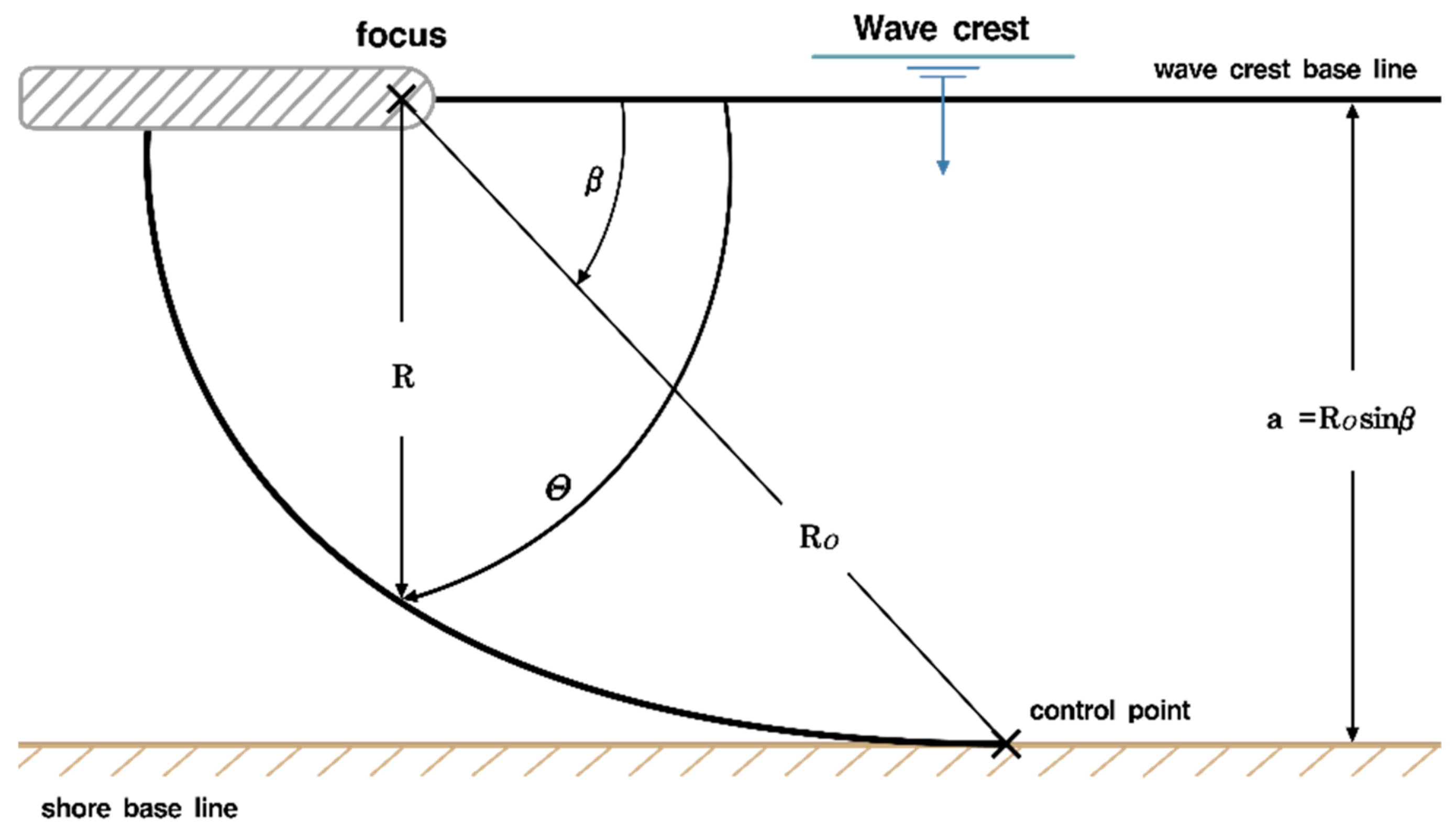
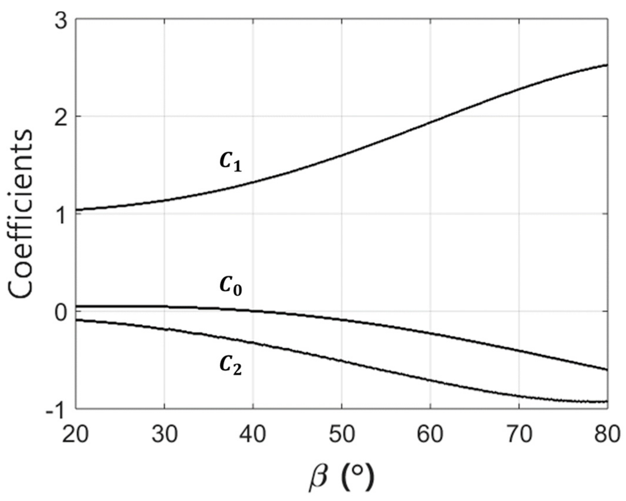
Here, refers to the radical distance from the parabolic focus to the shoreline, refers to the offshore distance between the wave crest baseline that passes the focus and the shore baseline that passes the control point in parallel, refers to the angle between the wave crest baseline and a line that travels from the focus through the control point, refers to the angle between the wave crest baseline and a line that connects the focus with the equilibrium shoreline, and , and are fitting coefficients, as provided by Hsu and Evans [18], as displayed in Figure 2. The sum of the three fitting coefficients must equal 1, so that the bay sector and the linear sector may connect.
However, there are some obstacles for the direct application of original PBSE to actual coast. The major obstacle is the location of the control point considered as an unknown variable [44,45]. However, the shortcoming of PBSE was overcome by applying it to a polar coordinate system rather than Cartesian coordinate, simply by taking the upstream end of the littoral cell as the control point, and it produced similar results in sandy beaches around the world.
3.2. Improving Shoreline Change Model
To reflect the influence of wave diffraction exerted in the wake of a structure, the longshore sediment transport equation may be altered, as displayed in Equation (8).
Here, refers to the annual mean wave angle, and is given below in Figure 3 to include the effect of wave diffraction, which was obtained by an approximate formula of PBSE.
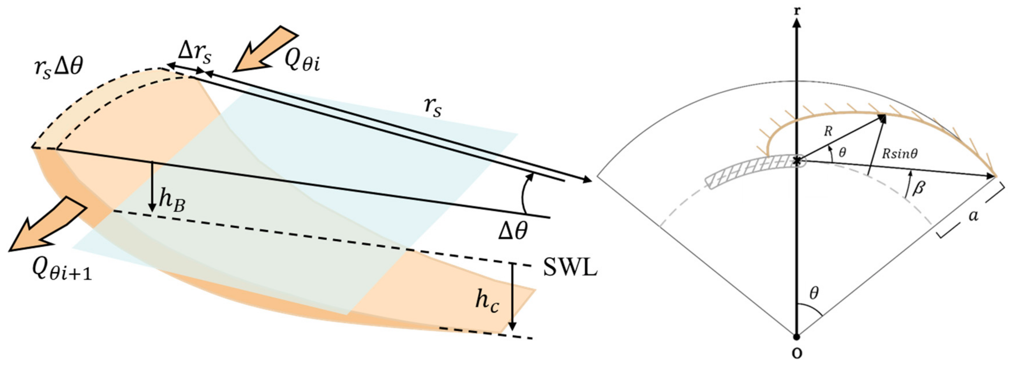
PBSE can be applied to the polar coordinate system for the circumference that fits the shoreline. By applying PBSE to the polar coordinate system, the applicability of the model to shorelines with curvature, such as a pocket beach, can be enhanced. Accordingly, applying Equation (5), as converted to the polar coordinate system, yields Equation (10).
Here, refers to the distance from the center of the circumference to the shoreline. The signs of which must be noted as it decreases if the shoreline advances, and increases if it retreats. Furthermore, can be calculated by using the PBSE-applied longshore sediment transport equation, as shown in Equation (10). Through this process, the effect of wave diffraction is reflected. refers to the longshore directional coordinate, and refers to longshore sediment transport in the direction of . Figure 4 illustrates the application of the polar coordinate system that fits the shape of the shoreline circumference.
Moreover, PBSE could be applied not only to shorelines, but also to depth contours as equipotential lines. The improved shoreline change model can also be applied to depth contours. Furthermore, when combined with the mean shoreline (MSL) response model for high waves of Yates et al. [46], the shoreline change simulation may be conducted with not only longshore sediment, but also cross-shore sediment during high waves.
The depth contour change model assumes that the beach profile does not alter its form but advances or retreats evenly. Namely, it is assumed that what governs the change to potential lines is not so much the alteration of the berm by cross-shore sediment transport, but the alteration of the berm by longshore sediment transport. Similar to the governing equation that determines the location of the shoreline, the difference in the sediment transport along the shore through the width between different depths yields Equation (11).
Here, refers to the sediment transport that flows through the width between depths within a specific period, which is estimated from the results of the wave model that is calculated at positions, unlike the shoreline change model.
3.3. Finite Difference Applied to Shoreline Change Model
The finite difference applied to the shoreline change model is presented in Figure 5. The beach is split into sectors along the shore, and it is assumed that the sediment transport increases or decreases in a sector according to the loss or inflow of sediment that occurs in the sector along the shore.
Using a ‘staggered grid’ in which {} and {} are defined crosswise as in the grid (i refers to the grid number), the sediment transport, , along the shore that applies finite difference is defined on the border of each grid, whereas the location of the shoreline is defined at the center of the grid. For convenience in expressing the difference equation, superscript n + 1 refers to the unknown value in the next time phase, and n is defined as the known value in the current time phase. Therefore, the location of the shoreline in n + 1, the next time phase in the i-th grid, may be expressed as in Equation (12).
Here, refers to the time interval, and refers to the longshore grid. can calculate the longshore sediment transport that converges to equilibrium by using Equation (8).
As for changes in depth contours, Equation (10) can be easily expanded to a finite difference equation. Longshore sediment transport, , is defined on the border of each grid, whereas the location of a depth contour is defined at the center of the grid, as expressed in Equation (13).
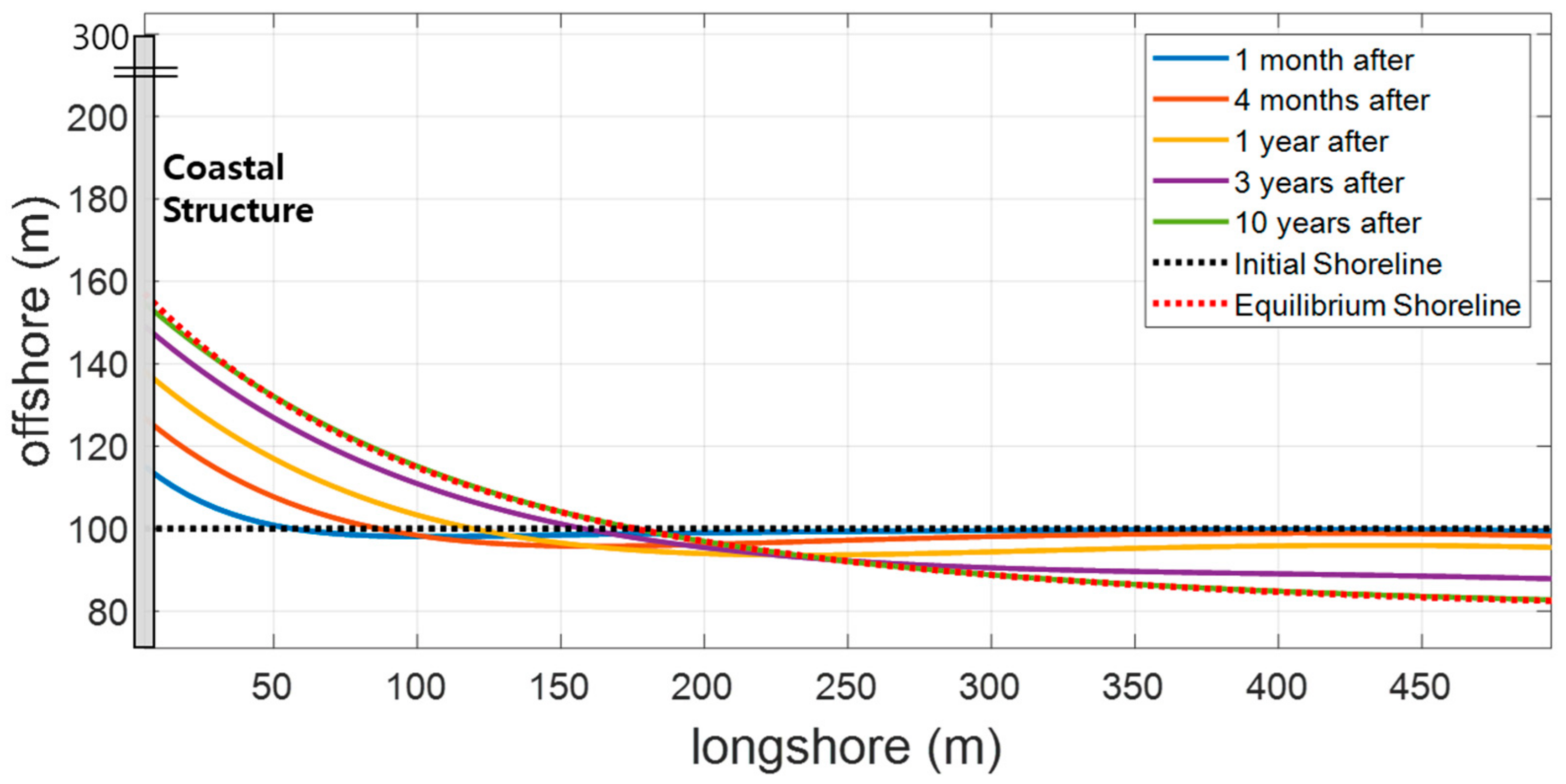
As discussed earlier, the explicit method uses past values to obtain the newly determined location of a shoreline. may be arbitrarily configured, where the longer it is configured, the shorter the calculation time becomes. However, choosing too large a value could compromise numerical and physical accuracy. Hence, a value between 6 and 24 h is widely used. Figure 6 displays the temporal change in which the shoreline changes following the installation of a seaport and offshore structures converge to the equilibrium shoreline (red dotted line), as per Hsu and Evans [18]. The equilibrium shoreline is a result of setting the ends (0, 300) of the structure as foci and applying the PBSE. The total sediment is conserved by blocking the longshore sediment transport rate, , in two end grids ().
Additionally, the shoreline change model enables the simulation of shoreline change due to the blocking system of longshore sediments, such as a groin. Figure 7 displays a simulation of shoreline change by setting the longshore sediment transport rate at the 1/4 point of the shoreline, , to 0. At this time, simulation is possible even in the case of a permeable structure by controlling the longshore sediment transport rate.
3.4. Theoretical Comparison with GENESIS Model
Hanson and Kraus [37] established the GENESIS model as a one-line shoreline change model derived from the shallow-water wave theory. Unlike the PBSE-applied shoreline change model, the GENESIS model considers wave diffraction in the second term. This section compares the results of the coastal erosion width caused by construction of coastal structures between the GENESIS model and the proposed model. Using the wave data at the position where a wave breaks due to a change in wave height in the longshore direction because of offshore structures, GENESIS expresses the longshore sediment transport as displayed in Equation (14).
In the second term, the shoreline transforms into the logarithmic-spiral curve in the diffracted wavefields, as suggested by Yasso [17]. However, underestimation is generally suspected when comparing to the results of actual shoreline changes. In contrast, the one-line shoreline change model presented in Section 3.3 demonstrated excellent reproducibility with convergence to the equilibrium shoreline, as displayed in Figure 6.
Additionally, as an approach to compare the GENESIS solution in Equation (14), Equation (8) is used to perform separation as below.
An approximation was made to make it resemble the GENESIS solution. Equation (17) was obtained for comparison.
Here, denotes the correction factor or function designed to make the GENESIS outcome converge to the equilibrium shoreline. The rate of change in the breaking wave height in the longshore direction is separated into a rate of change as affected by the diffraction direction of wave height, as displayed in Equation (18).
Here, refers to the angle defined between the endpoint of the offshore structure and the wave crest baseline and has become non-dimensional with . The tilde refers to the value lying outside the scope of the diffracted wave. The rate of change in the direction of , as affected by , is expressed as , the shortest distance from the initial shoreline to the endpoint of the offshore structure, as in Equation (19) when the parabolic equilibrium shoreline formula was applied.
acquires an approximate solution from the parabolic equilibrium shoreline formula as in Equation (20).
Therefore, when the results of the above equations were applied, the correction factor, , was derived as in Equation (21).
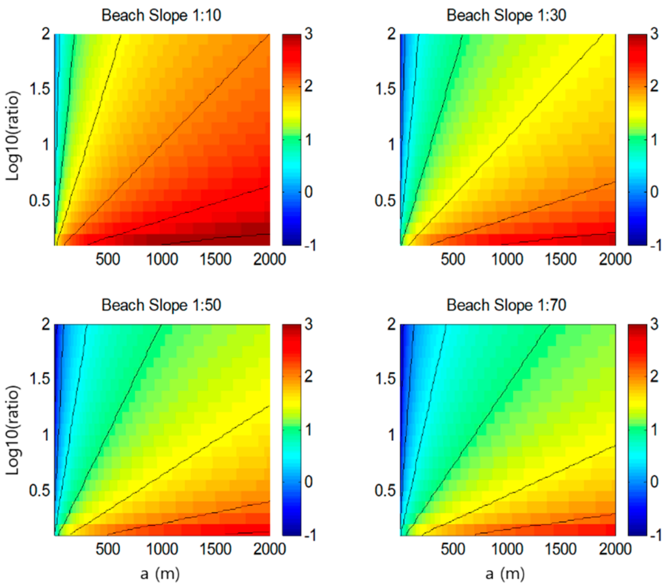
Here, the average beach slope, , obtains a value that is larger than 1 but smaller than 100. Except for the function of , whose influence from the result of Equation (21) is relatively small, the order of the correction factor, , was determined by the offshore distance, , and incident wave height. . Figure 8 illustrates the respective values of the correction factor,, against and according to the average beach slope. Increasing the offshore distance, , shows that the GENESIS model becomes the more underestimated results in shoreline deformation when compared with those of the present study.
4. Application of Shoreline Change Model in Republic of Korea
4.1. Site Description
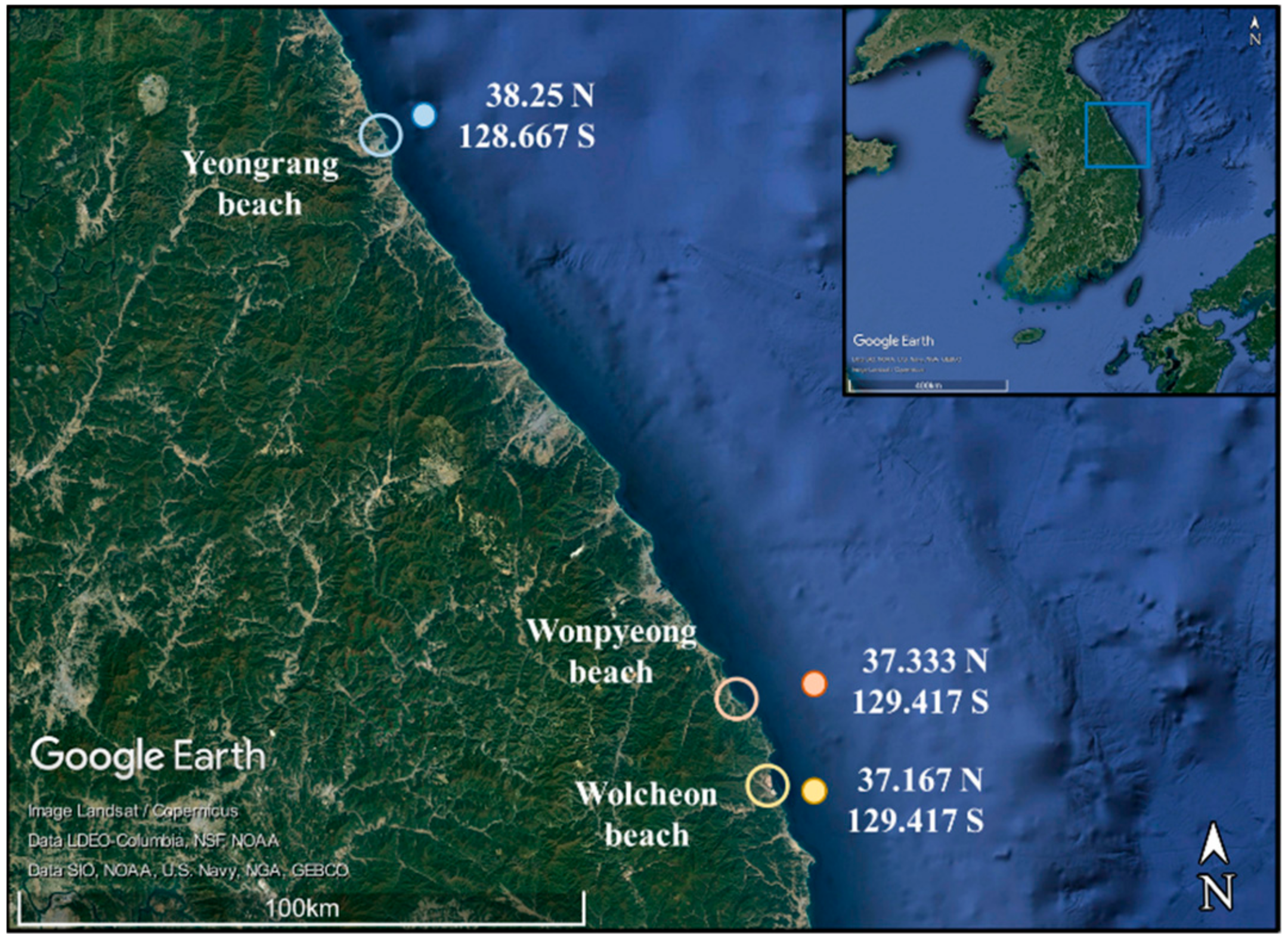
In this chapter, the proposed model was applied to the following three beaches on the east coast of Korea: Wonpyeong, Yeongrang, and Wolcheon beaches. These three studied sites underwent significant erosion damage after the construction of large-scale structures. The wave characteristics of the studied sites were analyzed using wave hindcast dataset provided by the wave information network of Korea [48]. Figure 9 shows a location map of the studied sites for model application, and of corresponding regions for wave hindcast dataset.
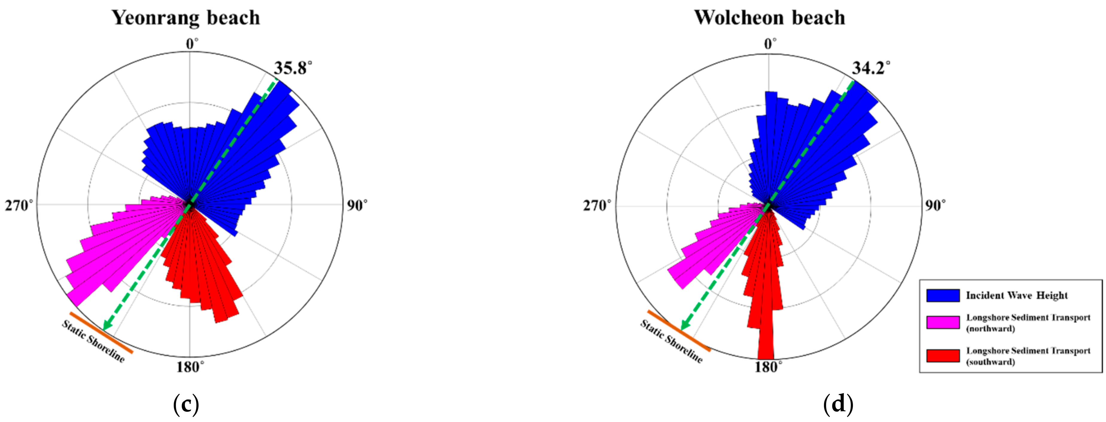
The root mean square (rms) wave heights of Wonpyeong, Yeongrang, and Wolcheon beaches were obtained to be 1.15, 1.04, and 1.00, respectively. Figure 10 shows the rose diagram of wave component (blue color) and corresponding longshore sediment transport components (purple color: northward, red color: southward) obtained from the wave hindcast data. Here, the angle of longshore sediment transport component, , is what (180 is added to wave angle, , as depicted in Figure 10a. The static equilibrium was achieved in the shore angle where the longshore sediment transport rate was in balance. The incident wave angles, , corresponding to the static equilibrium are shown in Figure 10; for Wonpyeong beach, for Yeongrang beach, and for Wolcheon beach. Therefore, if the wave angle, , is larger than the aforementioned values for , longshore sediment transport proceeds northward alongshore. However, if the value is smaller, it proceeds in the opposite direction.
4.2. Erosion of Wonpyeong Beach Caused by Construction of Gungchon Port
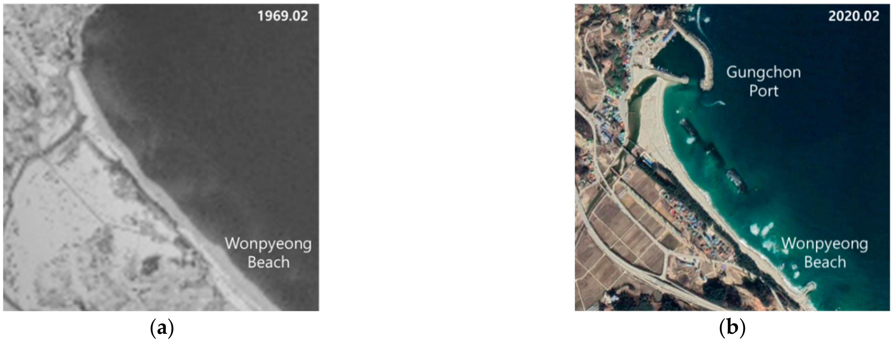
Located in Samcheok, Gangwon-do, Gungchon Port (construction started in 2000 and completed in 2012) is an outstanding case of coastal erosion caused by longshore sediment transport triggered by the construction of seaport structures. The construction of Gungchon Port gave rise to a change in the wavefield, as the sand lying south of the Wonpyeong beach moved closer to Gungchon Port. However, as the Gungchon Port’s breakwater and sand groin were built too close to one another, they failed to stop longshore sediment transport and a large quantity of sand moved north and accumulated in the southern side of a sand groin due to the longshore sediment transport when compared to before the construction of Gungchon Port (Figure 11). Figure 12 displays the outcome of simulation with the shoreline and depth contour change model as a result of the construction of Gungchon Port (run time (yr): 10, space elements: 100, and K value: 0.77). The simulation results confirm that, over time, the sand on the southern beach slowly moved north, thus converging to the coast that looks like what it is today.
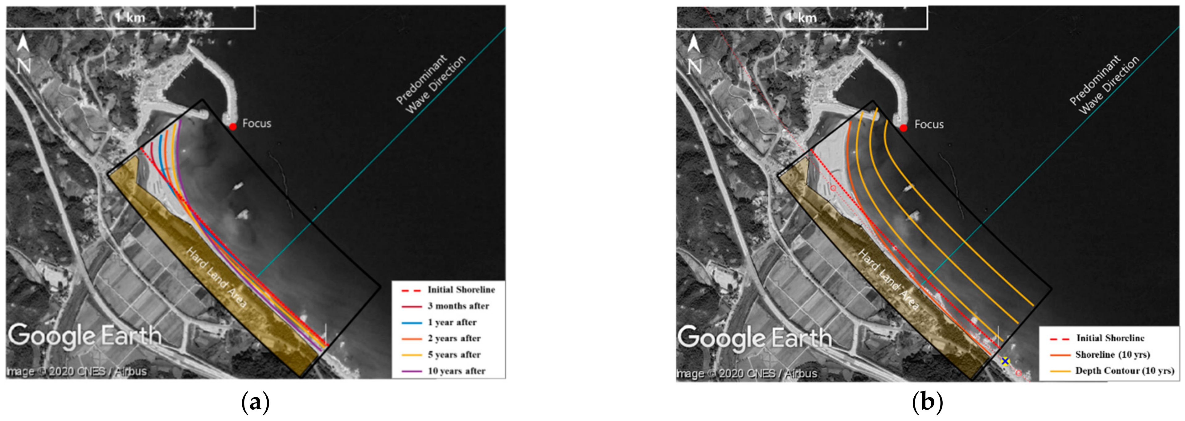
4.3. Erosion of Yeongrang Beach by Construction of Double Headland
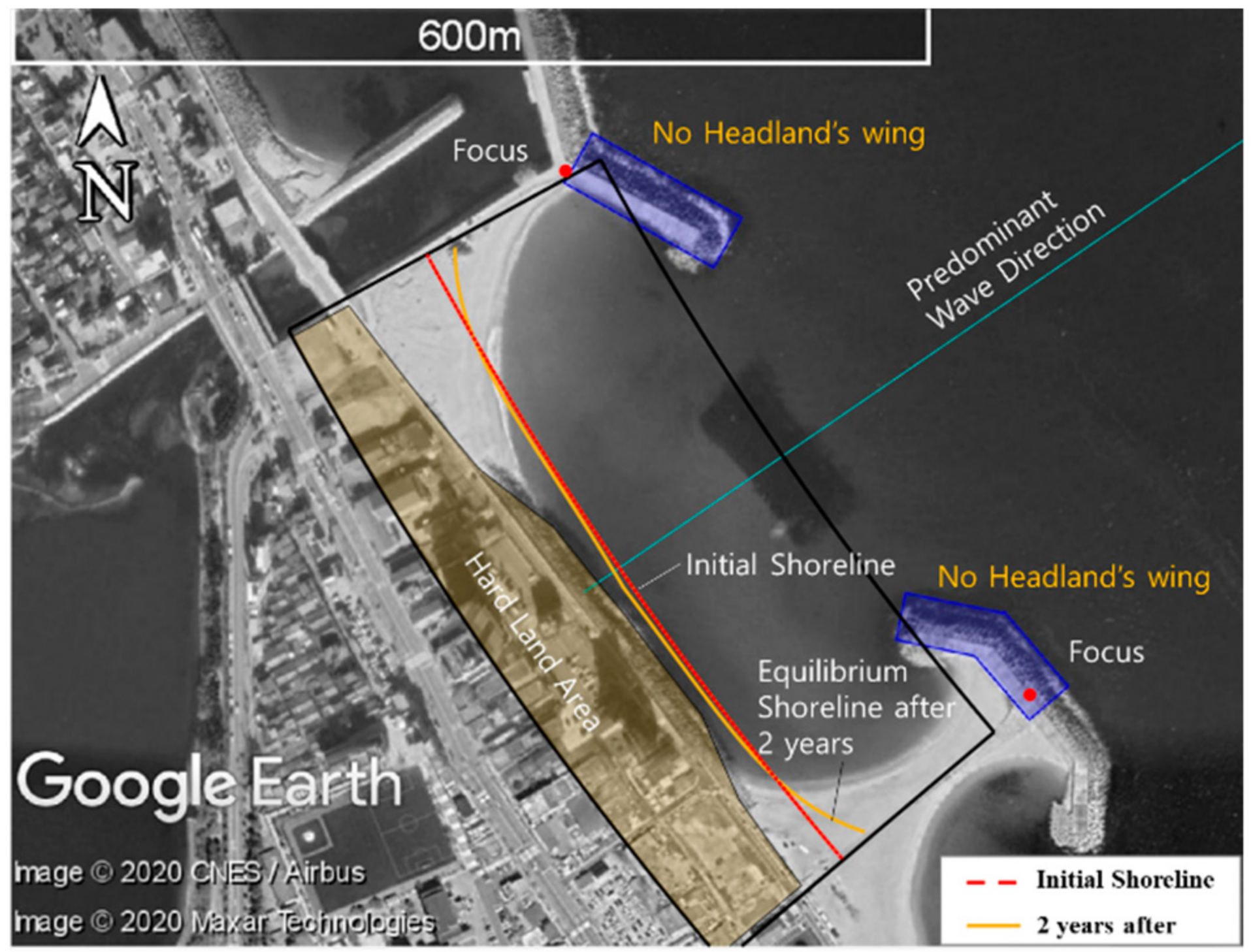
A double headland was installed at the Yeongrang beach in Sokcho, Gangwon-do, to mitigate the beach erosion problem caused after the construction of Jangsa Port (started in 2001 and completed in 2011). However, the construction of the double headland induced a significant erosion at the center of the beach, as displayed in Figure 13. The headland caused a change to the SEP of the beach, and the sand at the center eventually moved toward headlands on both ends. Figure 14 shows the model results of how the construction of the double headland affected the initial shoreline by gradually moving the sand at the center toward both ends (run time (yr): 2, space elements: 100, and K value: 0.77).
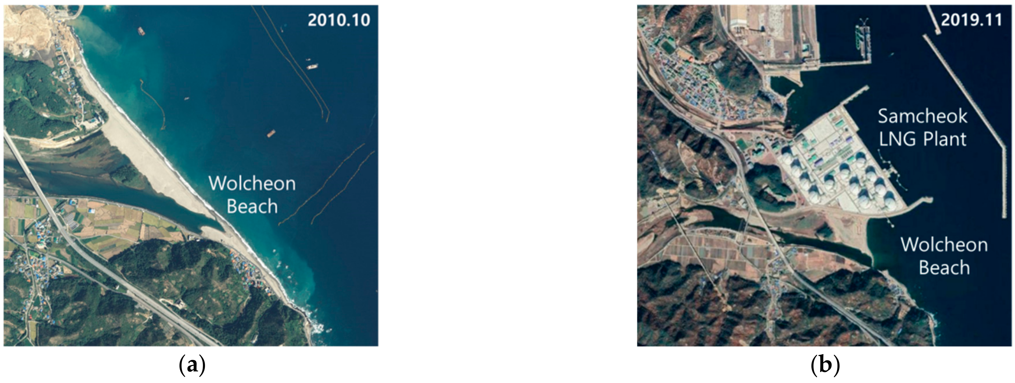
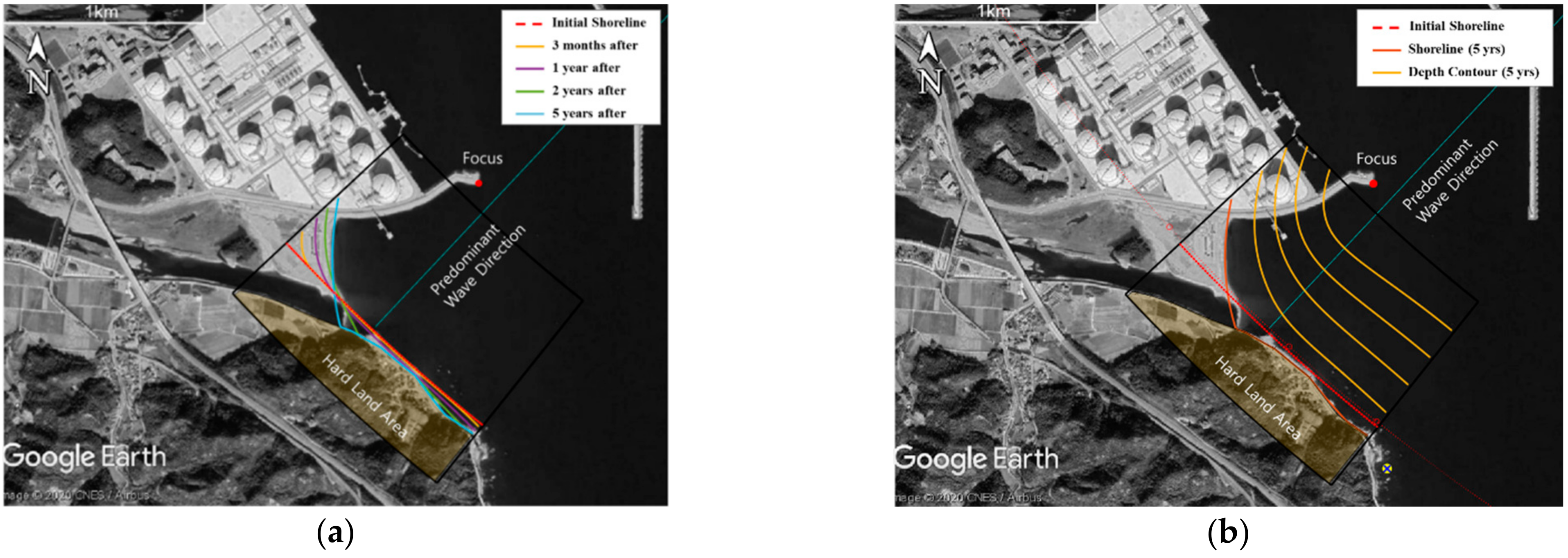
4.4. Erosion of Wolcheon Beach as Caused by Construction of Samcheok LNG Plant
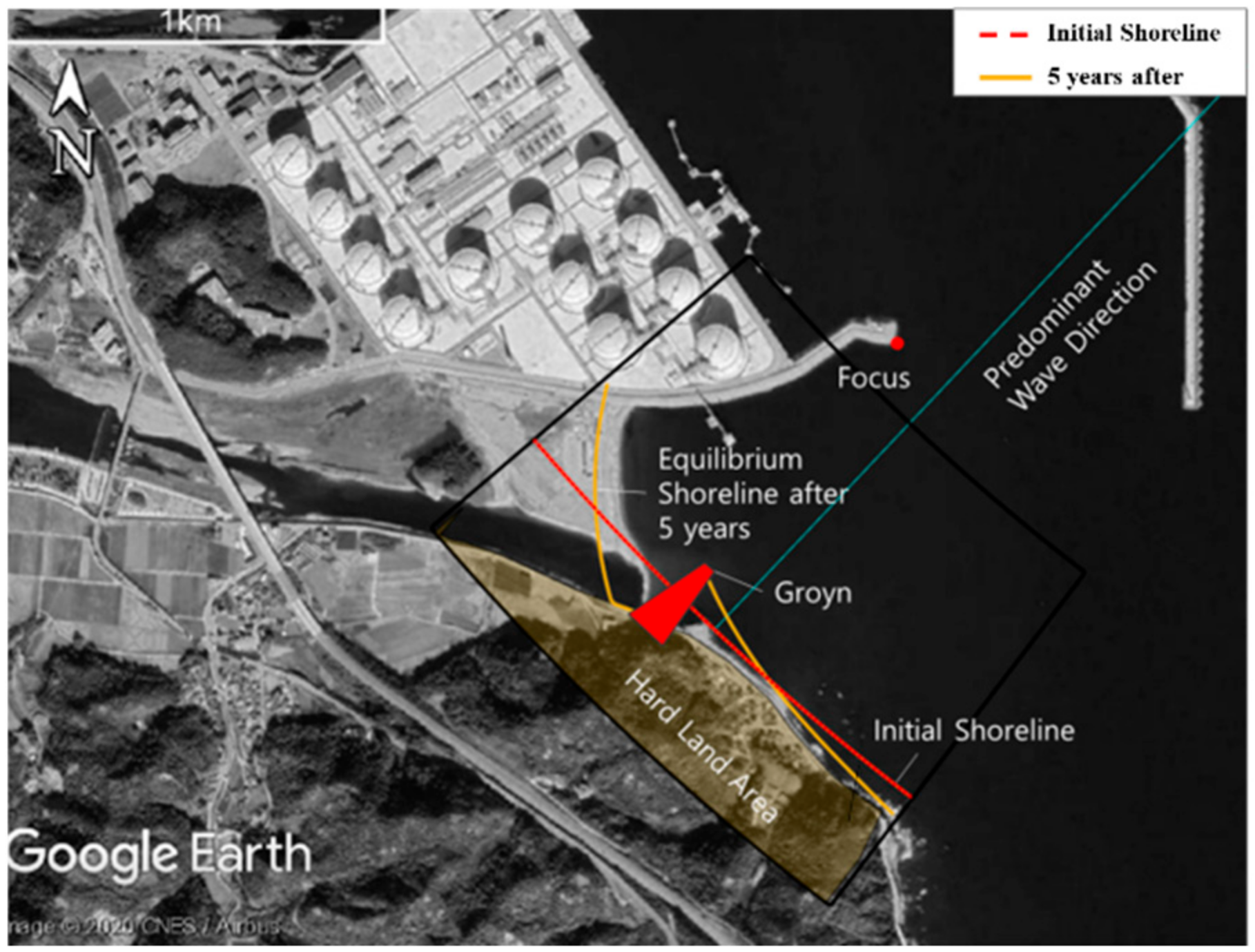
The Wolcheon beach in Samcheok, Gangwon-do was a long stretch of beautiful sandy beach approximately ten years ago (Figure 15a). Since the development of the Samcheok LNG Plant (construction started in 2008 and completed in 2017), it sucked most of the sand up, stripping the beach of its previous appearance (Figure 15b). The Samcheok LNG Plant significantly caused wave diffraction and consequently resulted in the clockwise rotation of SEP due to northward movement of sand. In Figure 16, the model simulation displays that just five years after the construction of the plant, most of the sand was accumulated in the estuary area (run time (yr): 5, space elements: 100, and K value: 0.77).
5. Discussion
5.1. Importance of Sand Groin Location for the Construction of Gungchon Port
As Gungchon Port continuously caused the erosion of the Wonpyeong beach, not only were three submerged breakwaters built near the port, but a groin was also built to the south of the beach belatedly, as displayed in Figure 11b. These measures did not prove to be too effectual, as offshore structures were built rashly without correctly understanding SEP. The principal cause of the erosion of the Wonpyeong beach was the absence of structures that could block the longshore sediment transport caused by Gungchon Port. While the sand groin could perform this function, it lay too close to the breakwater to play a significant role. The belatedly installed groin again lay too far from Gungchon Port to function properly, and any advancement of the shoreline was impossible. The simulation results demonstrated that if a groin or sand groin was placed in a quiet location, as displayed in Figure 17, it could maintain a portion of the sand near the port and keep sand on the beach (run rime (yr): 10, space elements: 100, and K value: 0.77). Therefore, the shoreline needs to be maintained by performing sand replenishment in the area affected by erosion and placing a groin in an appropriate location. Here, an overly long protrusion of a groin may cause a new equilibrium shoreline, which demands caution.
5.2. Mild Blocking of Incident Waves in the Construction Plan of Double Headland
To restore sand by reducing the waves at the center of the Yeongrang beach, a submerged breakwater was installed in the middle of the double headland (Figure 13b). While it was able to control high waves, it failed to change the equilibrium shoreline on the beach. Namely, the construction of the submerged breakwater was not as effective, as it failed to serve as a fundamental solution to the erosion. The fundamental cause was the overly large wings of the headland installed on the beach, which formed a new equilibrium shoreline. Instead of serving to block longshore sediment transport caused by the construction of Jangsa Port, it caused further damage from erosion. As displayed in Figure 18, a simulation with the model suggests that if the double headland lacks wings, several of the centers may suffer erosion, but it can maintain sand by serving to block longshore sediment transport (run time (yr): 2, space elements: 100, and K value: 0.77). In cases where it is difficult to remove those wings from the double headland, the center of the shoreline needs to be advanced with beach nourishment.
5.3. Pre-Installation of a Groin before Construction of Samcheok LNG Plant
To block the longshore sediment transport caused by the construction of the Samcheok LNG Plant, shore perpendicular structures such as groins or headlands need to be built in advance. Figure 19 displays the results of the model simulation of the shoreline change, assuming the construction of a groin to stop the longshore sediment transport from the construction of the Samcheok LNG Plant (run time (yr): 5, space elements: 100, and K value: 0.77). As a groin blocks sand movement, a portion of the sand, most of which has already disappeared, could be maintained. Thus, the model can be used to ensure the appropriate placement of groins to block longshore sediment transport caused by the construction of large seaport structures and offshore structures.
6. Conclusions
While there may be various reasons, a major cause of erosion is the change to wavefields as a result of the installation of offshore and seaport structures, which causes shoreline changes. Much research has been conducted on the model of shoreline change caused by changes in the coastal environment. However, such models were ineffective because of the uncertainty involved in how a shoreline converges to an equilibrium shoreline. Various studies have been performed on the equilibrium shoreline, but virtually none of the shoreline change models have been applied to target shorelines that should converge to them. Of all the empirical formulas for the equilibrium shoreline, the PBSE suggested by Hsu and Evans [18] is the one that has been most widely used, since its practicality and accuracy was confirmed. Hence, it was adopted in this study as well.
The shoreline change model that was developed in this study applies the longshore sediment transport formula of CERC [5] and is designed to converge to PBSE so that it may closely shadow natural shorelines. The model can simulate not only shorelines, but also changes to depth contours incurred when inputting the positions of control points set for different depths. Additionally, it can simulate the shoreline change after the construction of a structure that can block longshore sediment transport, such as a groin. Thus, the model can be widely used for coastal management. Today, many submerged structures such as submerged breakwaters, are built around the world, but the model presented in this study may be applied only to emergent structures. In addition, the present shoreline change model was developed to be simulated on satellite or aerial images. Therefore, it is suitable for preliminary study and pre-design in coastal engineering without laborious pre-process.
Author Contributions
Supervision, J.L.L.; Writing—Original draft, C.L.; Writing—Review & editing, C.L., J.L., and J.L.L. All authors have read and agreed to the published version of the manuscript.
Funding
This research was funded by the Ministry of Oceans and Fisheries, grant number 20180404, Korea.
Institutional Review Board Statement
Not applicable.
Informed Consent Statement
Not applicable.
Data Availability Statement
Not applicable.
Conflicts of Interest
The authors declare no conflict of interest.
References
- Kang, Y.K.; Park, H.B.; Yoon, H.S. Shoreline Changes Caused by the Construction of Coastal Erosion Control Structure at the Youngrang Coast in Sockcho, East Korea. J. Korean Soc. Mar. Environ. 2010, 13, 296–304. [Google Scholar]
- Longuet-Higgins, M.S. Longshore currents generated by obliquely incident sea waves, 1. J. Geophys. Res. 1970, 75, 6778–6789. [Google Scholar] [CrossRef]
- Longuet-Higgins, M.S. Longshore currents generated by obliquely incident sea waves, 2. J. Geophys. Res. 1970, 75, 6790–6801. [Google Scholar] [CrossRef]
- Komar, P.D.; Inman, D.L. Longshore and transport on beaches. J. Geophys. Res. 1970, 75, 5914–5927. [Google Scholar] [CrossRef]
- CERC (Coastal Engineering Research Center). Shore Protection Manual, 4th ed.; U.S. Army Engineers Waterways Experiment Station, Coastal Engineering Research Center, U.S. Government Printing Office: Washington, DC, USA, 1984. [Google Scholar]
- Kamphius, J.W. Alongshore transport of sand. In Proceedings of the 28th Coastal Engineering Conference, Cardiff, UK, 7–12 July 2002; ASCE: Reston, VA, USA, 1976; pp. 2478–2490. [Google Scholar]
- Bayram, A.; Larson, M.; Hanson, H. A new formula for the total longshore sediment transport rate. Coast. Eng. 2007, 54, 700–710. [Google Scholar] [CrossRef]
- Van Wellen, E.; Chadwick, A.J.; Bird, P.A.D.; Bray, M.; Lee, M.; Morfett, J.C. Coastal sediment transport on shingle beaches. In Proceedings of Coastal Dynamics ′97; American Society of Civil Engineers: Plymouth, MA, USA, 1997; pp. 38–47. [Google Scholar]
- Chastan, M.A.; Rosati, J.D.; McCormick, J.W.; Randall, R.E. Engineering Design Guidance for Detached Breakwaters as Shoreline Stabilization Structures; Technical Report CERC-93-19; US Army Engineers, Waterways Experiment Station, Coastal Engineering Research Center: Washington, DC, USA, 1993. [Google Scholar]
- Shinohara, K.; Tsubaki, T. Model study on the change of shoreline of sandy beach by the offshore breakwater. In Proceedings of the 10th Coastal Engineering Conference, Tokyo, Japan, 4–6 September 1966; pp. 551–563. [Google Scholar]
- Rosen, D.D.; Vajda, M. Sedimentological influences of detached breakwaters. In Proceedings of the 18th Coastal Engineering Conference, Cape Town, South Africa, 14–19 November 1982; ASCE: Reston, VA, USA, 1982; pp. 1930–1949. [Google Scholar]
- Suh, K.D.; Dalrymple, R.A. Offshore breakwaters in laboratory and field. J. Waterw. Port Coast. Ocean Eng. 1987, 113, 105–121. [Google Scholar] [CrossRef]
- Daohua, M.; Yee, M. Shoreline Changes behind Detached Breakwater. J. Waterw. Port Coast. Ocean Eng. 2000, 126, 63–70. [Google Scholar]
- Silvester, R.; Hsu, J.R.C. Coastal Stabilization: Innovative Concepts; Prentice-Hall: Englewood Cliffs, NJ, USA, 1993; p. 578. [Google Scholar]
- Silvester, R.; Hsu, J.R.C. Coastal Stabilization; Reprint of Silvester and Hsu, 1993; World Scientific: Singapore, 1997; p. 578. [Google Scholar]
- Hsu, J.R.C.; Uda, T.; Silvester, R. Shoreline protection methods—Japanese experience. In Handbook of Coastal Engineering; Herbich, J.B., Ed.; McGrawHill: New York, NY, USA, 2000; pp. 9.1–9.77. [Google Scholar]
- Yasso, W.E. Plan geometry of headland bay beaches. J. Geol. 1965, 73, 702–714. [Google Scholar] [CrossRef]
- Hsu, J.R.C.; Evans, C. Parabolic bay shapes and applications. Proc. Inst. Civ. Eng. 1989, 87, 557–570. [Google Scholar] [CrossRef]
- Moreno, L.J.; Kraus, N.C. Equilibrium shape of headland-bay beaches for engineering design. In Proceedings of Coastal Sediments ′99; American Society of Civil Engineers: New York, NY, USA, 1999; Volume 1, pp. 860–875. [Google Scholar]
- USACE. Coastal Engineering Manual; US Army Corps of Engineers: Washington, DC, USA, 2002. Available online: http://chl.erdc.usace.army.mil/chl.aspx?p_s&a_articles;104 (accessed on 30 April 2002).
- Herrington, S.P.; Li, B.; Brooks, S. Static Equilibrium Bays in Coast Protection; Marine Engineering Group, Institution of Civil Engineers: London, UK, 2007. [Google Scholar] [CrossRef]
- Bowman, D.; Guillén, J.; López, L.; Pellegrino, V. Planview geometry and morphological characteristics of pocket beaches on the Catalan coast (Spain). Geomorphology 2009, 108, 191–199. [Google Scholar] [CrossRef]
- González, M.; Medina, R.; Losada, M.A. On the design of beach nourishment projects using static equilibrium concepts: Application to Spanish coast. Coast. Eng. 2010, 57, 227–240. [Google Scholar] [CrossRef]
- Silveira, L.F.; Klein, A.H.F.; Tessler, M.G. Headland-bay beach platform stability of Santa Catarina State and the northern coast of São Paulo State. Braz. J. Oceanogr. 2010, 58, 101–122. [Google Scholar] [CrossRef]
- Yu, J.T.; Chen, Z.S. Study on headland-bay sandy cast stability in South China coasts. China Ocean Eng. 2011, 25, 1. [Google Scholar] [CrossRef]
- Anh, D.T.K.; Stive, M.J.F.; Brouwer, R.L.; de Vries, S. Analysis of embayed beach platform stability in Danang, Vietnam. In Proceedings of the 36th IAHR World Congress, The Hague, The Netherlands, 28 June–3 July 2015; p. 6. [Google Scholar]
- Thomas, T.; Williams, A.T.; Rangel-Buitrago, N.; Phillips, M.; Anfuso, G. Assessing embayment equilibrium state, beach rotation and environmental forcing influences: Tenby Southern Wales, UK. J. Mar. Sci. Eng. 2016, 4, 30. [Google Scholar] [CrossRef] [Green Version]
- Ab Razak, M.S.; Jamaluddin, N.; Mohd Nor, N.A.Z. The platform stability of embayed beaches on the west coast of Peninsular Malaysia. JESTEC 2018, 80, 33–42. [Google Scholar]
- Ab Razak, M.S.; Mohd Nor, N.A.Z.; Jamaluddin, N. Platform stability of embayed beaches on the east coast of Peninsular Malaysia. JESTEC 2018, 13, 435–448. [Google Scholar]
- Lim, C.B.; Lee, J.L.; Kim, I.H. Performance test of parabolic equilibrium shoreline formula by using wave data observed in East Sea of Korea. J. Coast. Res. 2019, 91, 101–105. [Google Scholar] [CrossRef]
- Pelnard-Considere, R. Essai de Theorie de l’Evolution des Formes de Rivage en Plages de Sable et de Galets. Journ. Hydraul. 1957, 4, 289–298. [Google Scholar]
- Bakker, W.T. The Dynamics of a Coast with a Groyne System. In Proceedings of the 11th International Conference on Coastal Engineering, London, UK, 16 September 1968; pp. 492–517. [Google Scholar]
- Hulsbergen, C.H.; Bakker, W.T.; van Bochove, G. Experimental Verification of Groyne Theory. In Proceedings of the 15th International Conference on Coastal Engineering, Honolulu, HI, USA, 11–17 July 1976; ASCE: Reston, VA, USA, 1976; pp. 1439–1458. [Google Scholar]
- Le Mehaute, B.; Soldate, M. Mathematical Modelling of Shoreline Evolution; Misc. Rpt. 77-10; U.S. Army Corps of Engineers, Coastal Engineering Research Center: Washington, DC, USA, 1977; p. 56. [Google Scholar]
- Walton, T.L.; Chiu, T.Y. A Review of Analytical Techniques to Solve the Sand Transport Equation and Some Simplified Solutions. In Proceedings of Coastal Structures ’79; ASCE: Reston, VA, USA, 1979; pp. 809–837. [Google Scholar]
- Larson, M.; Hanson, H.; Kraus, N.C. Analytical Solutions of the One-Line Model of Shoreline Change; Tech. Report CERC-87-15; U.S. Army Corps of Engineers, Coastal Engineering Research Center: Washington, DC, USA, 1987. [Google Scholar]
- Hanson, H.; Kraus, N.C. Genesis: Generalized Model for Simulating Shoreline Change; U.S. Army Corps of Engineers, Coastal Engineering Research Center: Washington, DC, USA, 1989. [Google Scholar]
- Leont’yev, I.O. Short-Term Shoreline Changes Due to Cross-Shore Structures: A One-Line Numerical Model. Coast. Eng. 1997, 31, 59–75. [Google Scholar] [CrossRef]
- Leont’yev, I.O. Changes in the Shoreline Caused by Coastal Structures. Oceanology 2007, 47, 877–883. [Google Scholar] [CrossRef]
- Vaidya, A.M.; Kori, S.K.; Kudale, M.D. Shoreline Response to Coastal Structures. Aquat. Procedia 2015, 4, 333–340. [Google Scholar] [CrossRef]
- Ozasa, H.; Brampton, A.H. Math-ematical modeling of beaches backed by sea-walls. Coast. Eng. 1980, 4, 47–64. [Google Scholar] [CrossRef]
- Gallerano, F.; Cannata, G.; Scarpone, S. Bottom changes in coastal areas with complex shorelines. Eng. Appl. Comput. Fluid Mech. 2017, 11, 396–416. [Google Scholar] [CrossRef]
- Klonaris, G.; Memos, C.D.; Droenen, N.; Deigaard, R. Boussinesq-Type Modeling of Sediment Transport and Coastal Morphology. Coast. Eng. J. 2017, 59, 1750007-1–1750007-27. [Google Scholar] [CrossRef]
- Lausman, R.; Klein, A.H.F.; Stive, M.J.F. Uncertainty in the application of parabolic bay shape equation: Part 1. Coast. Eng. 2010, 57, 132–141. [Google Scholar] [CrossRef]
- Lausman, R.; Klein, A.H.F.; Stive, M.J.F. Uncertainty in the application of parabolic bay shape equation: Part 2. Coast. Eng. 2010, 57, 142–151. [Google Scholar] [CrossRef]
- Yates, M.L.; Guza, R.T.; O’Reilly, W.C. Equilibrium shoreline response: Observations and modeling. J. Geophys. Res. 2009, 116. [Google Scholar] [CrossRef] [Green Version]
- Lee, J.L.; Hsu, J.R.C. Numerical Simulation of Dynamic Shoreline Changes Behind a Detached Breakwater by Using an Equilibrium Formula. In Proceedings of the International Conference on Offshore Mechanics and Arctic Engineering, Trondheim, Norway, 25–30 June 2017. [Google Scholar]
- Jeong, W.; Oh, S.; Ryu, K.; Back, J.; Choi, I. Establishment of Wave Information Network of Korea (WINK). J. Korean Soc. Coast. Ocean Eng. 2018, 30, 326–336. [Google Scholar] [CrossRef] [Green Version]
Figure 1.
Definition sketch of parabolic model for bay-shaped beach.

Figure 2.
Coefficients of parabolic bay shape equation [18].
Figure 2.
Coefficients of parabolic bay shape equation [18].

Figure 3.
Definition sketch of annual mean wave angle and gradient of equilibrium shoreline.

Figure 4.
Concept diagram for shoreline change model as applied to polar coordinate system.

Figure 5.
Numerical analysis of shoreline change model.

Figure 6.
Shoreline change model of convergence to equilibrium shoreline.

Figure 7.
Simulation of shoreline change after construction of groin.

Figure 8.
Correction factor against offshore distance and incident wave height (w.r.t 1:10, 1:30, 1:50, and 1:70) [47].
Figure 8.
Correction factor against offshore distance and incident wave height (w.r.t 1:10, 1:30, 1:50, and 1:70) [47].

Figure 9.
Location of studied sites and hindcast wave data.

Figure 10.
Rose diagram of wave and longshore sediment transport with respect to incident angle: (a) definition sketch, (b) Wonpyeong beach, (c) Yeongrang beach, and (d) Wolcheon beach.
Figure 10.
Rose diagram of wave and longshore sediment transport with respect to incident angle: (a) definition sketch, (b) Wonpyeong beach, (c) Yeongrang beach, and (d) Wolcheon beach.


Figure 11.
Changes at Wonpyeong beach before and after construction of Gungchon Port: (a) February 1969 (image from NGII(National Geographic Information Institute)); (b) February 2020 (image from Google Earth).
Figure 11.
Changes at Wonpyeong beach before and after construction of Gungchon Port: (a) February 1969 (image from NGII(National Geographic Information Institute)); (b) February 2020 (image from Google Earth).

Figure 12.
Shoreline change model simulation of change to Wonpyeong beach, caused by construction of Gungchon Port: (a) shoreline change; (b) depth contour change (image from Google Earth as at October 2012).
Figure 12.
Shoreline change model simulation of change to Wonpyeong beach, caused by construction of Gungchon Port: (a) shoreline change; (b) depth contour change (image from Google Earth as at October 2012).

Figure 13.
Yeongrang beach before and after construction of double headland: (a) October 2005 (image from NGII); (b) April 2015 (image from NGII).
Figure 13.
Yeongrang beach before and after construction of double headland: (a) October 2005 (image from NGII); (b) April 2015 (image from NGII).

Figure 14.
Shoreline change model simulation of change to Yeongrang beach, caused by construction of double headland: (a) shoreline change; (b) depth contour change (image from Google Earth as at April 2019).
Figure 14.
Shoreline change model simulation of change to Yeongrang beach, caused by construction of double headland: (a) shoreline change; (b) depth contour change (image from Google Earth as at April 2019).

Figure 15.
Wolcheon beach before and after construction of Samcheok LNG Plant: (a) October 2010 (image from NGII); (b) November 2019 (image from Google Earth).
Figure 15.
Wolcheon beach before and after construction of Samcheok LNG Plant: (a) October 2010 (image from NGII); (b) November 2019 (image from Google Earth).

Figure 16.
Shoreline change model simulation of change that construction of Samcheok LNG Plant caused to Wolcheon beach: (a) shoreline change; (b) depth contour change (image from Google Earth as at November 2019).
Figure 16.
Shoreline change model simulation of change that construction of Samcheok LNG Plant caused to Wolcheon beach: (a) shoreline change; (b) depth contour change (image from Google Earth as at November 2019).

Figure 17.
Results of model simulation to reduce erosion of Wonpyeong beach by repositioning groin (image from Google Earth as at October 2012).
Figure 17.
Results of model simulation to reduce erosion of Wonpyeong beach by repositioning groin (image from Google Earth as at October 2012).

Figure 18.
Results of model simulation, supposing that the double headland’s wings are removed (image from Google Earth as at April 2019).
Figure 18.
Results of model simulation, supposing that the double headland’s wings are removed (image from Google Earth as at April 2019).

Figure 19.
Shoreline change model simulation of prevention of loss of sand from Wolcheon beach through construction of groin (image from Google Earth as at November 2019).
Figure 19.
Shoreline change model simulation of prevention of loss of sand from Wolcheon beach through construction of groin (image from Google Earth as at November 2019).

Publisher’s Note: MDPI stays neutral with regard to jurisdictional claims in published maps and institutional affiliations. |
© 2021 by the authors. Licensee MDPI, Basel, Switzerland. This article is an open access article distributed under the terms and conditions of the Creative Commons Attribution (CC BY) license (http://creativecommons.org/licenses/by/4.0/).
Share and Cite
MDPI and ACS Style
Lim, C.; Lee, J.; Lee, J.L. Simulation of Bay-Shaped Shorelines after the Construction of Large-Scale Structures by Using a Parabolic Bay Shape Equation. J. Mar. Sci. Eng. 2021, 9, 43. https://doi.org/10.3390/jmse9010043
AMA Style
Lim C, Lee J, Lee JL. Simulation of Bay-Shaped Shorelines after the Construction of Large-Scale Structures by Using a Parabolic Bay Shape Equation. Journal of Marine Science and Engineering. 2021; 9(1):43. https://doi.org/10.3390/jmse9010043
Chicago/Turabian StyleLim, Changbin, Jooyong Lee, and Jung Lyul Lee. 2021. "Simulation of Bay-Shaped Shorelines after the Construction of Large-Scale Structures by Using a Parabolic Bay Shape Equation" Journal of Marine Science and Engineering 9, no. 1: 43. https://doi.org/10.3390/jmse9010043
Note that from the first issue of 2016, this journal uses article numbers instead of page numbers. See further details here.