Optimal Damping Concept Implementation for Marine Vessels’ Tracking Control


Computer Applications and Systems Department, Saint-Petersburg State University, Universitetskii Prospekt 35, Petergof, 198504 Saint Petersburg, Russia
J. Mar. Sci. Eng. 2021, 9(1), 45; https://doi.org/10.3390/jmse9010045
Submission received: 26 November 2020
/
Revised: 29 December 2020
/
Accepted: 29 December 2020
/
Published: 4 January 2021
(This article belongs to the Special Issue Automatic Control and Routing of Marine Vessels)
Abstract
:This work presents the results of studies related to the design of stabilizing feedback connections for marine vessels moving along initially given trajectories. As is known, in mathematical formalization, this question leads to a problem of tracking control synthesis for nonlinear and non-autonomous plants. To provide desirable stability and performance features of the closed-loop systems to be synthesized, it is appropriate to use an optimization approach. Unlike the known synthesis methods, which are usually used within the framework of this approach, it is proposed to implement the optimal damping concept first developed by V.I. Zubov in the early 60s of the last century. Modern interpretation of this concept allows constructing numerically effective procedures of control law synthesis taking into account its applicability in a real-time regime. Central attention is focused on the questions connected with practical adaptation of the optimal damping methods for marine control systems. The operability and effectiveness of the proposed approach are illustrated by a practical example of tracking control design.
1. Introduction
The nonlinear tracking control of modern marine vessels is one of the most practically significant and theoretically considerable problems in the area of automatic control analysis and design. In particular, tracking control systems are widely used in different branches such as hydrography, inspection of marine constructions, wreck investigation, underwater cable laying, and so on [1,2]. Central theoretical and practical background of tracking control for various moving plants is presented in [3,4,5] and other fundamental works.
Various issues associated with the design of tracking controllers for marine surface vessels have already been extensively researched and presented in numerous publications (for example, [1,2,6,7,8,9,10,11,12,13,14,15,16]). To evaluate the state of the art in marine tracking control, let us address some modern works presenting this direction of research.
Currently, it is possible to use various ideas to design nonlinear tracking control laws that are reflected in numerous publications, for example, [7,8,13,14,15,16]. However, let us note that the mentioned works are not directly oriented to the application of the optimization technique. This makes it difficult to provide the desired dynamic features of the closed-loop connections. Now, it seems to be quite evident that the most effective analytical and numerical tool for feedback connections design is the optimization approach. Several aspects of nonlinear tracking control optimization technique are presented in multitudinous scientific publications, including such popular monographs as [4,5,17,18,19,20,21]. As for the simplest stabilization problem, the autopilots with multipurpose structures of optimized control laws are discussed in detail in [22,23,24,25,26].
The sliding mode control technique for marine control applications is discussed in [1,2,6,8]. This direction seems to be quite constructive, but poorly applicable, since it leads to intensive wear of the actuators.
As for the model predictive control (MPC) approach [9], its most significant disadvantage is the large dimension of the minimization problem that is solved at each step of the control process.
Notably, the complexity of this problem is vast because of the many dynamic requirements, restrictions, and conditions that must be satisfied by the chosen control actions.
It should be noted that many scientific works devoted to the tracking control for marine vessels use linear time invariant models of their motion. However, such models are not quite adequate for the problems of deep maneuvering control in angle and positional dynamic variables. Respectively, one of the most important practical difficulties requiring consideration in the design process is the account of nonlinearity and non-autonomy of the control plant model. In most cases, this problem is a source of dynamic instability and poor performance for various systems that were designed based only on linear approximations.
As for the aforementioned optimization approach, its advantages are determined by the flexibility and convenience of modern optimization methods with respect to the relevant practical demands for control design implementation. Certain analytical and numerical methods are used now to compute the optimal controllers for nonlinear and non-autonomous systems subject to various given performance indices. Nevertheless, there is no saying that the optimization approach is recognized overall as a universal instrument to be put into practice for marine tracking controllers design. This can be explained by the presence of some disadvantages connected with computational troubles. Therefore, there exists a vital necessity to develop persistently analytical and numerical methods of control laws design based on optimization ideology adapting to the specific problems for various marine applications.
At present time, numerous approaches are used for a practical solution of these problems [1,2,3,4,5,6,7,8,9,10,11,12,17,18]. Usually, they are based on Pontryagin’s maximum principle, on Bellman’s dynamic programming principle, on finite-dimensional approximation in the range of model predictive control (MPC) technique, etc. Unfortunately, all these approaches are connected with the huge extent of calculations that essentially impedes their implementation both for laboratory design activity and real-time regimes of control.
The existence of numerical difficulties motivates us to use other approaches that allow avoiding the aforementioned shortcomings. This work focuses on a different concept that can be applied to design tracking controllers using the theory of optimal damping (OD). This theory, which was first proposed and developed by V.I. Zubov in his works [19,20,21], provides effective analytical and numerical methods for control calculations with essentially reduced computational consumptions with respect to classical techniques. We believe that this theory was ahead of its time and was undeservedly underutilized for practical control problem solving. This work is one of the attempts to overcome this omission, taking into account the impressive development of modern computer technologies.
In this article, special attention is paid to the control of marine vessels in terms of the forward speed and heading angle. We are considering the regime of the acceleration in order to achieve the specified forward speed with one-time turn along the heading. To achieve desirable stability and performance features of the reference motion, the correspondent tracking controllers were designed based on the OD technique.
The main contribution of this paper is determined by the following statements. First, we propose to use the OD concept to design tracking controllers for marine vessel speed and heading. This has not been the case before. Second, we discuss a new methodology for selecting the functional to be damped, taking into account the desirable features of the closed-loop system in the range of the optimization technique. Hereby, the choice of this functional as the basis is argued by the guarantee asymptotic stability and the desired quality of control processes. Third, we point to the possibility of applying the OD approach to a wide class of nonlinearities in the mathematical model of the vessel. It is noted that this approach can be implemented in real-time regime of a ship’s motion. The practical applicability and effectiveness of the proposed technique is illustrated by a controller design for a transport marine ship.
The novelty of the proposed approach with respect to other works lies in the universality and flexibility of proposed nonlinear non-autonomous control laws based on OD computational procedure, which can be implemented in a real-time regime of functioning for marine control plants.
In general, the present study is an extension of the multipurpose approach proposed in [22,23,24,25,26,27] and developed in [28] with respect to the marine autopilot control laws with the novel structure, taking into account actuators’ time delays.
This article is organized as follows. In Section 2, the optimal damping concept for control law synthesis for nonlinear non-autonomous systems is discussed, taking into account certain specific stability and performance requirements for marine control applications. The known background is presented, and the novel ways are proposed to provide tracing controllers synthesis. Section 3.1 is devoted to the OD synthesis problem statement for the forward speed tracking controller and for the tracking autopilot. Central attention is paid to the presentation of mathematical models of the control plant and dynamic requirements for the quality of the closed-loop connection. Section 3.2 presents an exhaustive novel solution for the mentioned synthesis problem based on the optimal damping concept. In Section 3.3, a practical example of tracking controller synthesis is presented to illustrate the applicability and effectiveness of the proposed approach. Finally, Section 4 concludes the article by discussing the overall results of the investigation and indicates how these results can be further developed.
2. Materials and Methods
As mentioned above, the essence of this paper involves developing an optimal damping technique of tracking control law synthesis for marine vessels with nonlinear and non-autonomous models. In this section, let us first consider the background and some essential features of the OD approach that define the methodological basis of the study.
First of all, let us introduce a commonly used nonlinear robot-like model of the control plant, which represents marine vessel motion for various regimes of its operation [1,2,6]:
where vector presents velocities defined in a plant-fixed frame and vector contains position dynamical parameters (displacements and angles) in an Earth-fixed frame. External disturbances and controls are presented by the vectors and , respectively. Let us accept that the inertia matrix is positive definite: , the matrix of Coriolis-centripetal terms is skew-symmetrical: , and the damping matrix is positive definite but non-symmetrical. Vector represents gravitational and buoyancy forces and moments, is the matrix of rotations, and the matrix with the constant components reflects controls allocation.
Let us provide a transformation of the body-fixed frame representation (1) to the Earth-fixed one with respect to the vector . Following [1], this can be done using the following notations:
In accordance with (2), initial model (1) of the plant takes the form:
The essence of the tracking control problem is to provide given desirable motion of the vessel, using the following state feedback
which is a nonlinear non-autonomous tracking controller.
Within mathematical formalization, controller (4) must be implemented to provide the zero equilibrium with respect to the tracking error for the closed-loop system (3), (4), where . Naturally, this equilibrium point must be asymptotically stable to guarantee that as . Let us especially note that the mentioned closed-loop system is nonautonomous, if we have no constant reference motion . This gives reasons for us to require the uniform asymptotic stability in global (UGAS) or local (UAS) form. An additional requirement is that the controller (4) provides the desired dynamical features for the closed-loop system (3), (4) under the action of an admissible control .
To set the perform of the controller (4) synthesis, we assume that the vector functions , , and the corresponding are given. These functions satisfy Equations (1) or (3), i.e., we have:
Let introduce the following additional notations:
which allows us to present Equations (1) and (5) as
supposing that .
Let us also consider deflections
of the vessel dynamical parameters from the desirable motion.
Then, we can present equations of the vessel in the deflections from the desirable motion. Using notations (7) on the base of (6), we obtain
where
It is a matter of simple calculations to check that equation (6) has zero equilibrium position, which must be stabilized by the choice of the controller . If this controller is found, then the tracking feedback (4) can be presented as
As for the desirable dynamic features of the closed-loop connection, the most widely used formalized approach is based on minimizing the following integral functional:
that determines the quality of control processes for a closed-loop system. Here, subintegral function is positive definite, i.e., However, as is well known, there are certain difficulties in directly implementing this approach, which are determined by the huge extent of calculations that essentially impedes their practical implementation.
We propose to overcome the mentioned obstacles using a novel technique based on the OD concept, connected to the OD problem for the synthesis of the control . To state this problem, firstly, let us introduce the functional to be damped as follows:
where is a Lyapunov function candidate, and is a positively defined function. Let us additionally accept that the function satisfies the following conditions:
where are comparison functions [4].
The essence of the OD approach consists of the control generation as a function from the current values of variables in the form
where is the metric compact set, and is a rate of the functional change along the motions of the plant (8):
In other words, it is necessary to find OD controller (13), using an admissible set such that .
We can specify three possible ways to solve this optimization problem:
- (a)
- The first way is based on the direct numerical calculation of the vectors providing the pointwise minimization of the function by the choice of for current points . Let us especially notice that this variant is universal in nature and can be applied to generate a control signal for real-time regime of motion.
- (b)
- The second way involves the possibility of an analytical solution to the problem (13). Naturally, this is the most preferred way, but such a situation is quite rare, although an example of its practical application will be given below.
- (c)
- The third way reduces the problem (13) to a numerical solution of a nonlinear system of finite equations. In fact, if we have , then with necessity we obtain
Using the necessary condition (14), one can solve the following nonlinear system
for any point with respect to the vector , where , ,
3. Results
This section is devoted to a practical implementation of the proposed OD approach to nonlinear tracking controllers design for marine vessels. Particular attention is given to the forward speed tracking control law with initially given reference signal.
3.1. Tracking Control Problem for Marine Vessels
To consider the problems of tracking control for marine applications, let us accept the following widely used [1,2] nonlinear dynamical model of a marine vessel:
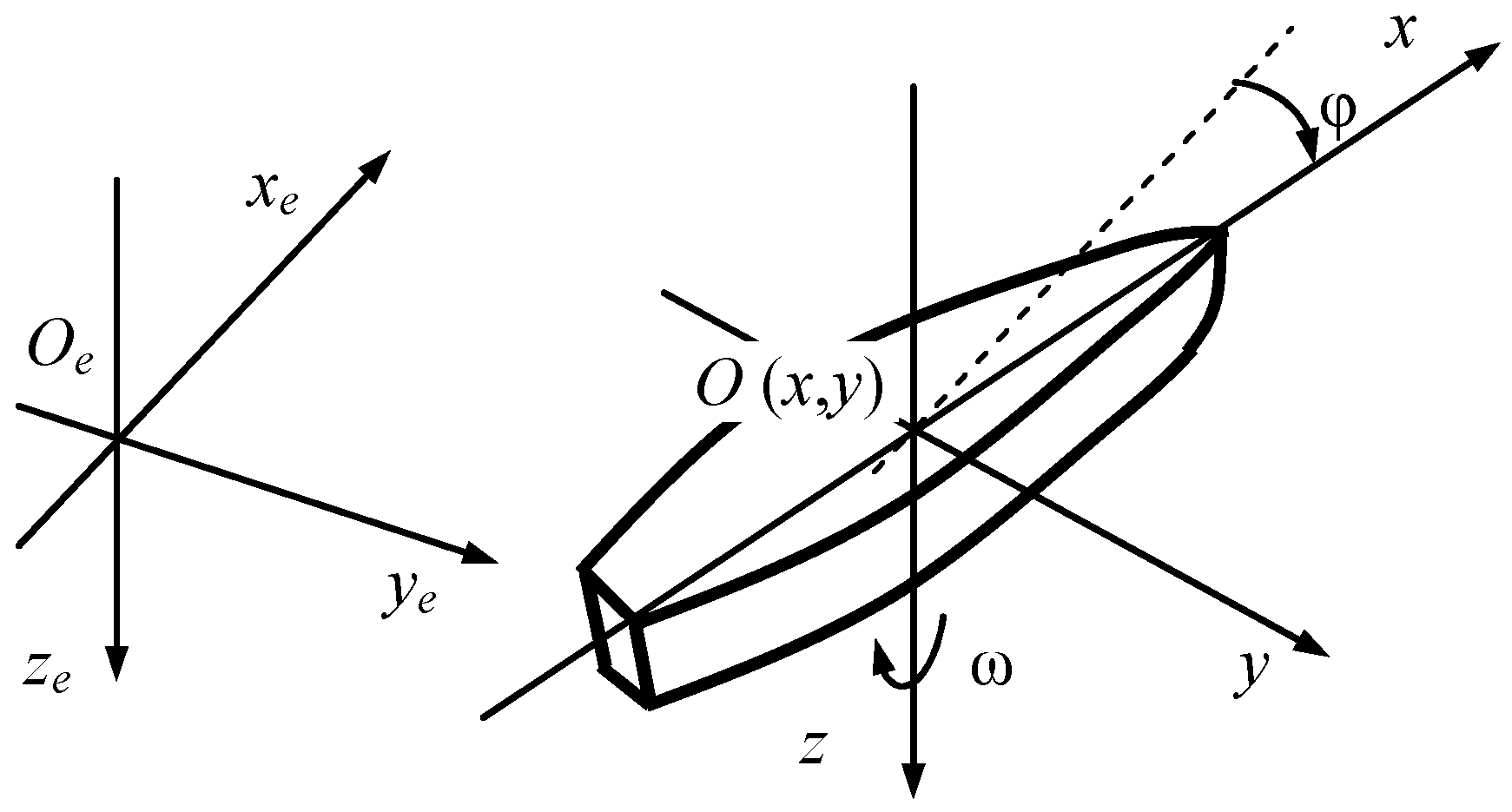
Here, the following notations are used: , and are the projections of the velocity vectors on the axes of a vessel-fixed frame (Figure 1); is the auxiliary vector of dynamical parameters; is the heading angle, and is the vertical rudder deflection. The functions and represent hydrodynamical forces, which are produced by the ship’s engine and the water resistance correspondingly.
The control signals and must be composed by the automatic control system to be designed. The first of them determines a reference surge speed of the vessel, and the second one presents a reference speed of the rudders’ deflections.
Assuming that the number of the screw rotations is proportional to a reference surge speed, the function determining a trust force of the screw can be presented in the form
We accept here that , and that the variables and are treated as known functions of the dynamical parameters .
Let us introduce new vector variables , , and, taking into account (16), we can rewrite nonlinear model (1) of the vessel dynamic as follows:
Now we specify a certain reference motion , , , and of the plant (17), satisfying the identities
Using systems (17) and (18), we can present equations of vessel dynamic in deflections from the desirable reference motion of the form
where
One can see that , , , and are known functions of : using new correspondent notations , we can rewrite (19) as follows:
stating that the resulting system (21) has a zero-equilibrium position.
Let us especially note that, unlike (17), this system is not only nonlinear, but also non-autonomous. This is due to the explicit introduction of the time-dependent reference signals into the vessel dynamics equations.
The purpose of the control design procedure is to construct the following stabilizing feedback controllers in deviations:
such that the zero equilibrium of the closed-loop connection (21), (22) is asymptotically stable. This means that if the motion of the initial plant (15) takes place under the action of tracking controllers of the form
starting in some neighborhood of the point , then this motion tends to the reference one as becomes infinite.
As for the performance of control processes, they are usually formalized mathematically using certain functionals, which are given on the motions of the closed-loop system (21), (22). Currently, the commonly used approach to design stabilizing controllers (22) is setting and solving the following optimization problem
based on the integral functional
where is the set of admissible pairs and subintegral function is positive definite for all its arguments.
In contrast to the problems (24), (25) with traditional methods of its solving, as mentioned above, we propose to use novel approach based on the OD concept.
Let us especially note that both the solution of the problem (24) and the solution of the OD problem significantly depend on the initially given mathematical model (21) of a marine vessel. Naturally, this is evidence that this model cannot be formed accurately, which raises very important questions about the robust features of the closed-loop system to be designed. This problem is quite solvable for various types of marine vessels: the paper [29] is an example. However, the study of the robust features of tracking OD controllers presents an independent problem to be addressed in future studies.
3.2. Forward Speed OD Tracking Controller Design
In general, the synthesis of the two stabilizing controllers (22) using OD technique can be carried out simultaneously. Nevertheless, one can also apply a combined approach to the feedback design for the considered plant (21) with two control channels. In the range of this approach, the first control is formed based on the OD problem, and the second one can be designed in any other way, providing desirable performance features. However, a joint closed-loop system must have zero equilibrium, and this motion must be asymptotically stable.
Realizing this idea, let us accept the dynamic controller for rudders (marine autopilot) in the following form:
where is the state vector of this controller.
In particular, the feedback (26) may have a multipurpose structure, which is presented in detail in [22,27] for linear time-invariant case. Its implementation taking into account control time-delay is investigated in the paper [28].
The equations of the control plant now take the form
In order to synthesize a feedback for the first control channel, i.e., design the OD forward speed stabilizing controller, let us introduce the functional to be damped as
Let us take as a Lyapunov function candidate the following sum of quadratic forms:
Based on (28), (29), we can state the correspondent OD problem of the form
where the rate of the functional change is determined as follows:
Let us solve the problem (30), taking into account (31) and assuming that the extreme is achieved at the inner point of the set : with necessity we obtain
that determines the following controller
Since, according to formulae (15)–(21), we have
we arrive from (32) at the following OD controller:
where , .
It is necessary to note that if the value is out of an inner part of the admissible set , we must use the control signal instead of (33).
It is necessary to note that practical problems involve situations where the right part of the equation for forward speed has a more complex structure than for the system (17). In general, this equation can be presented as
which results in the correspondent equation for the system (21) in deflections:
where In this case, instead of (31) we have
and the analytical search for stationary points of the function becomes problematic. Nevertheless, it is always possible to consider a question about the numerical solution of OD problem (30) for each aggregate of fixed parameters . Moreover, it is always possible to pose a finite dimensional minimization problem
on the finite net for any compact set . This problem should be solved at the time for the fixed parameters . Obviously, with a sufficiently large number of points for the set , the solution of the problem (34) tends to solution for the same problem on the set .
Finally, in accordance with formula (23), we can compose the tracking controller of the form
where the stabilizing part is determined by equality (33). One can see that the resulting representation for OD forward speed tracking controller is as follows:
The current values of the dynamic parameters must be measured to implement the controller (35).
3.3. Numerical Example of OD Tracking Controller Synthesis
To illustrate a practical implementation of the proposed OD approach, let us consider a practical example of forward speed tracking controller design for the transport ship with a displacement of 3500 tons, a length of 110 m, a width of 14 m, and an immersion of 5 m. As a mathematical model of the plant, let us accept equations (17), which are presented in [1,2] with the given functions , , and parameter .
First, we define the reference motion of the ship as a partial solution of system (17) with the initial conditions , . Let us accept the reference forward speed control as follows:
To determine the reference control for the rudders, let us initially construct a model feedback as a controller
fulfilling the command-heading signal . The basis item in (37) stabilizes Linear Time Invariant (LTI) plant
which is a result of the plant (17) linearization in the neighborhood of the origin for a fixed forward speed . Let us especially notice that the linear model (38) is used only for the synthesis of controller (37) but is not used for simulation and for performance indices computation: controller (37) closes full initial model (17) of the vessel.
Accepting , we obtain
We design the basis control for plant (38) with aforementioned parameters as the Linear Quadratic Regulator (LQR) optimal controller with respect to the functional
where , . Let us especially remark that the choice of the presented parameters for the functional (39) is determined by the initially given requirements to a dynamic quality of the control processes for the nonlinear time varying system. These requirements provide desirable settling time and overshoot for the closed-loop connection.
As a result of computations, we get the constant vector , where
Let us substitute the reference heading control and the rudders feedback control
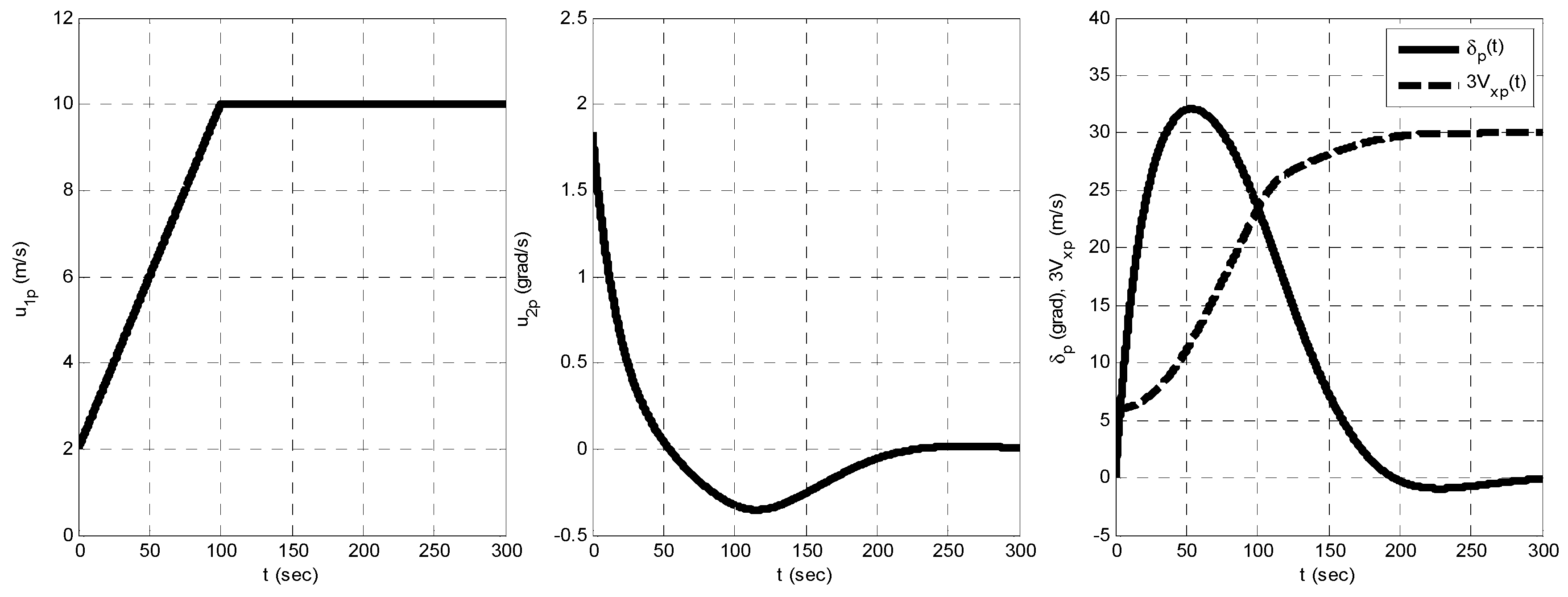
into Equation (17). After integration, we obtain the functions , , and , which determine given reference motion of the vessel. The graphs of aforementioned functions are presented in Figure 2 and Figure 3.
To provide simulation process, instead of (23), (26), we accept the following simple feedback control law for a marine autopilot:
where is the command-heading signal. This controller, corresponding to (40), can be directly used for actuators of the vertical rudders.
Thus, one can see that, as a result, initial control plant (17) is closed by the tracking controllers (35) and (41). The current values of the dynamic parameters , , , , and must be measured by the corresponding sensors for the actual implementation of these controllers.
For simulation of the closed-loop system dynamics, the following parameters values are accepted: , , , . In addition, let us take into account the restrictions and .
To illustrate the practical applicability of the proposed approach, let us simulate the control processes for the closed-loop connection. The aim is to make the proposed approach comparable to other methods. This determined the choice of design parameters and regimes of vessel’s motion. These regimes represent the most popular options for movement on quiet water and under the action of sea waves.
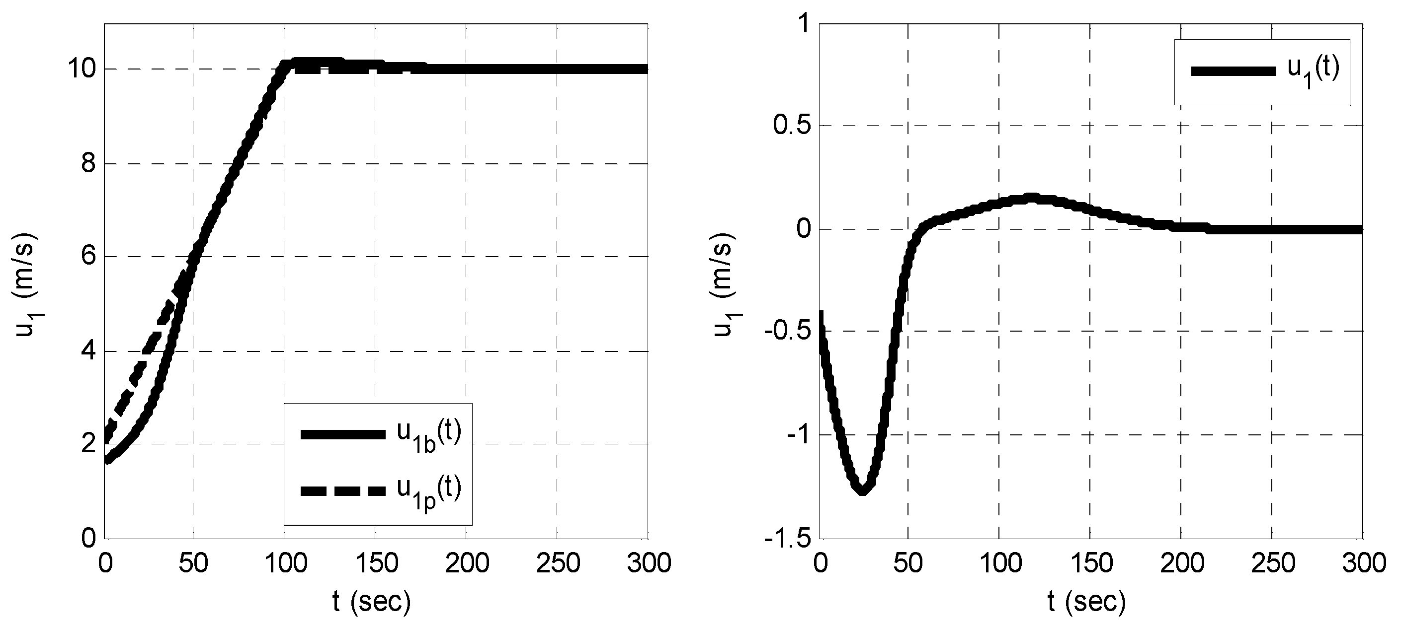
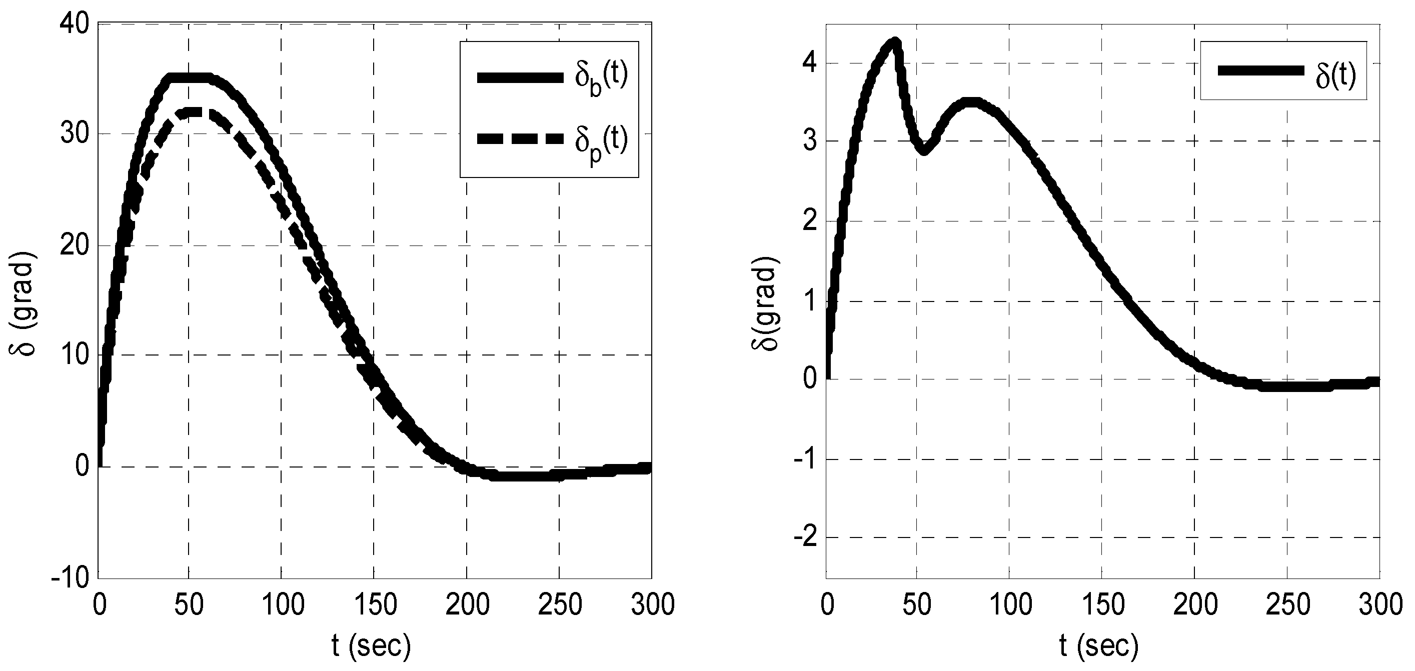
The results of simulation are presented in Figure 4, Figure 5 and Figure 6 as the graphs of corresponding functions, which reflect control signals and the vessel’s state variables for the transient process. This process is determined by the aforementioned reference motion, which is realized with the help of the designed tracking controllers. Initial conditions for all variables are zero with the exception of forward speed and heading angle. By these variables, the initial conditions and are accepted to distinguish them from the reference motion.
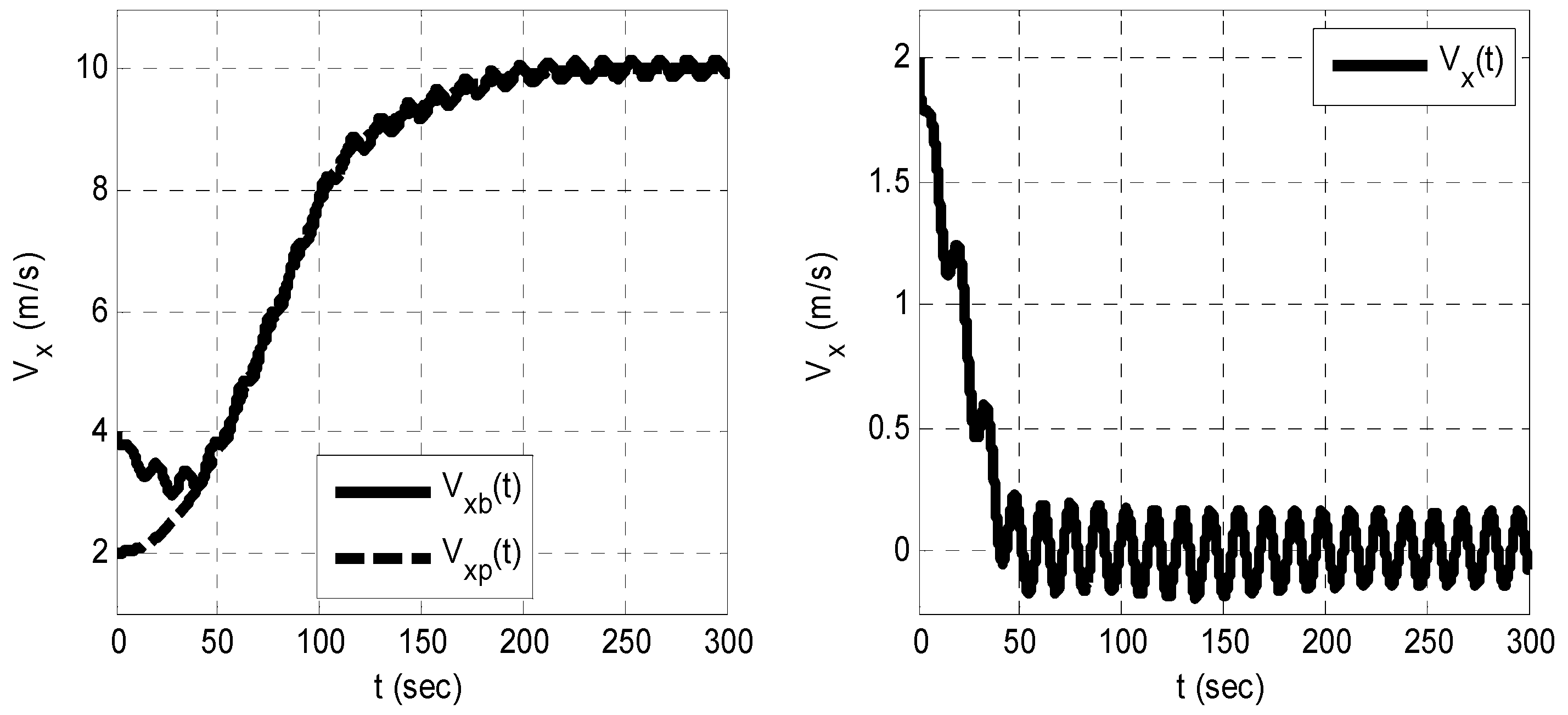
Let us note that the dynamical quality of the presented transient process seems to be quite satisfactory. In addition, it is suitable to illustrate the dynamics of the closed-loop connection under the action of sea wave external disturbance. Figure 7 shows the same control process for the forward speed , taking into account presence the approximate representation of sea waves with an intensity of 5 on the Beaufort scale.
Finally, let us analyze the stability of the closed-loop system (17), (35), (41) with synthesized tracking controllers. One can easily see that in order to provide aforementioned analysis, it is sufficient to consider the zero-equilibrium stability for the closed-loop system (27), (33) presented in deflections from the reference motion.
It is obvious that systems (27), (33) have zero equilibrium, and to investigate its stability features, let us introduces the following Lyapunov function candidate:
Here, the symmetrical matrix is a solution of the algebraic Riccati equation, which is used in the range of LQR controller (37) synthesis:
Let us notice that the introduced function satisfy the relationships
with the following -class functions:
where and are the minimum and maximum eigenvalues of the matrix , respectively.
Using the additional function , one can check if the following inequality is valid
where is a box, determined by the relationships:
Here, the variable determines the relative width of the box compared to the current values of the reference signals. This variable was increased to such a value that the condition (44) was met. The obtained value seems to be still admissible in the range of (43), (44) [4,5], determining the region of the local uniform asymptotic stability for the reference motion, which is realized by tracking controllers (35), (41).
4. Discussion
The main goal of this work was to propose constructive methods for marine tracking controllers’ design taking into account the real conditions of a vessel’s motions. We focused our main attention on a situation where the rudders’ deflections and the forward speed are presented by initially given reference signals to be realized using tracking feedback controls.
This problem can be solved using different popular optimization approaches (Bellman’s theory, MPC technique, sliding mode control, etc.). Nevertheless, we propose a new specific method for tracking controllers’ design, which ensures the desirable reference motion of the vessel along the forward speed and heading angle.
This method is based on the optimal damping concept, which has certain advantages related to the practical requirements for the dynamic features of a closed-loop connection. The main advantage of the aforementioned approach is that the numerical solution of the optimization problems is essentially simplified. In contrast to well-known approaches [1,2,3,4], we applied OD tracking feedback as a control law with special features that allow it to be adjusted and implemented in real-time regime of motion.
The main result of this study is the development of the optimal damping concept to ensure its practical applicability and effectiveness that is illustrated by a controller design for a transport ship.
The investigations presented above could be further developed to consider the robust features of the tracking control laws, information about the measurement noise, and the presence of transport delays [24]. The results of the executed research could also be implemented to provide desirable reference motion of the dynamic positioning systems for marine vessels [26,27]. Certain attention may be given to the multipurpose control laws applications [22,23,24,25]. As for direct development of this study, it is possible to also use OD controller for the vertical rudders. The extension of the proposed approach to various robotic systems is also of considerable interest. The scope of the proposed approach may additionally include remotely operated vehicles [11] and offshore structures [12].
Funding
This research was funded by the Russian Foundation for Basic Research (RFBR) controlled by the Government of Russian Federation, research project number 20-07-00531.
Acknowledgments
The author expresses his sincere gratitude to A.P. Zhabko for the interest to the topic of this study and for the high-level professional suggestions.
Conflicts of Interest
The authors declare no conflict of interest.
References
- Fossen, T.I. Guidance and Control of Ocean Vehicles; John Wiley & Sons Ltd.: New York, NY, USA, 1994. [Google Scholar]
- Do, K.D.; Pan, J. Control of Ships and Underwater Vehicles. Design for Underactuated and Nonlinear Marine Systems; Springer: London, UK, 2009. [Google Scholar]
- Jarjebowska, E. Model-Based Tracking Control of Nonlinear Systems; CRC Press, Taylor & Francis Group: Boca Raton, FL, USA, 2012. [Google Scholar]
- Khalil, H.K. Non-Linear Systems; Prentice Hall: Englewood Cliffs, NJ, USA, 2002. [Google Scholar]
- Slotine, J.; Li, W. Applied Nonlinear Control; Prentice Hall: Englewood Cliffs, NJ, USA, 1991. [Google Scholar]
- Fossen, T.I. Handbook of Marine Craft Hydrodynamics and Motion Control; John Wiley & Sons, Ltd.: New York, NY, USA, 2011. [Google Scholar]
- Reyes-Bayes, R.; Donaire, A.; van der Shaft, A.; Jayawardhana, B.; Perez, T. Tracking Control of Marine Craft in the port-Hamiltonian Framework: A Virtual Differential Passivity Approach. In Proceedings of the 17th European Control Conference (ECC 2019), Naples, Italy, 25—28 June 2019; pp. 1636–1641. [Google Scholar]
- Liu, Y.; Bu, R.; Gao, X. Ship Trajectory Tracking Control Systems Design Based on Sliding Mode Control Algorithm. Pol. Marit. Res. 2018, 25, 26–34. [Google Scholar] [CrossRef] [Green Version]
- Guerreiro, B.J.; Silvestre, C.; Cunha, R.; Pascoal, A. Trajectory tracking nonlinear model predictive control for autonomous surface craft. IEEE Trans. Control. Syst. Techol. 2014, 22, 2160–2175. [Google Scholar] [CrossRef]
- Hammound, S. Ship Motion Control Using Multi-Controller Structure. J. Marit. Res. 2012, 55, 184–190. [Google Scholar]
- Capocci, R.; Dooly, G.; Omerdi’c, E.; Coleman, J.; Newe, T.; Toal, D. Inspection-Class Remotely Operated Vehicles—A Review. J. Mar. Sci. Eng. 2017, 5, 13. [Google Scholar] [CrossRef]
- Ramos, R.L. Linear Quadratic Optimal Control of a Spar-Type Floating Offshore Wind Turbine in the Presence of Turbulent Wind and Different Sea States. J. Mar. Sci. Eng. 2018, 6, 151. [Google Scholar] [CrossRef] [Green Version]
- Roy, S.; Shome, S.N.; Nandy, S.; Ray, R.; Kumar, V. Trajectory Following Control of AUV: A Robust Approach. J. Inst. Eng. India Ser. C 2013, 94, 253–265. [Google Scholar] [CrossRef]
- Ye, J.; Roy, S.; Codjevac, M.; Baldi, S. A Switching Control Perspective on the Offshore Construction Scenario of Heavy-Lift Vessels. IEEE Trans. Control Syst. Technol. 2020, 29, 1–8. [Google Scholar] [CrossRef]
- He, W.; He, X.; Zoo, M.; Li, H. PDE Model-Based Boundary Control Design for a Flexible Robotic Manipulator With Input Backlash. IEEE Trans. Control Syst. Technol. 2019, 27, 790–797. [Google Scholar] [CrossRef]
- He, W.; Gao, H.; Zhou, C.; Yang, C. Reinforcement Learning Control of a Flexible Two-Link Manipulator: An Experimental Investigation. IEEE Trans. Syst. Man Cybern. Syst. 2020. [Google Scholar] [CrossRef]
- Lewis, F.L.; Vrabie, D.L.; Syrmos, V.L. Optimal Control; John Wiley & Sons, Ltd.: New York, NY, USA, 2012. [Google Scholar]
- Geering, H.P. Optimal Control with Engineering Applications; Springer-Verlag: Berlin/Heidelberg, Germany, 2007. [Google Scholar]
- Zubov, V.I. Oscillations in Nonlinear and Controlled Systems; Sudpromgiz: Leningrad, USSR, 1962. (In Russian) [Google Scholar]
- Zubov, V.I. Theory of Optimal Control of Ships and Other Moving Objects; Sudpromgiz: Leningrad, USSR, 1966. (In Russian) [Google Scholar]
- Zubov, V.I. Theorie de la Commande; Mir: Moscow, USSR, 1978. [Google Scholar]
- Veremey, E.I. Synthesis of multiobjective control laws for ship motion. Gyroscopy Navig. 2010, 1, 119–125. [Google Scholar] [CrossRef]
- Veremey, E.I. Dynamical Correction of Control Laws for Marine Ships’ Accurate Steering. J. Mar. Sci. Appl. 2014, 13, 127–133. [Google Scholar] [CrossRef]
- Veremey, E.I. Optimization of filtering correctors for autopilot control laws with special structures. Optim. Control Appl. Methods 2016, 37, 323–339. [Google Scholar] [CrossRef]
- Veremey, E.I. Special Spectral Approach to Solutions of SISO LTI H-Optimization Problems. Int. J. Autom. Comput. 2019, 16, 112–128. [Google Scholar] [CrossRef]
- Veremey, E.I. Separate Filtering Correction of Observer-Based Marine Positioning Control Laws. Int. J. Control 2017, 90, 1561–1575. [Google Scholar] [CrossRef]
- Sotnikova, M.V.; Veremey, E.I. Dynamic Positioning Based on Nonlinear MPC. IFAC Proc. Vol. (IFAC Pap.) 2013, 9, 31–36. [Google Scholar] [CrossRef]
- Veremey, E.I.; Pogozhev, S.V.; Sotnikova, M.V. Multipurpose Control Laws Synthesis for Actuators Time Delay. J. Mar. Sci. Eng. 2020, 8, 477. [Google Scholar] [CrossRef]
- Chen, M.; Ge, S.S.; How, B.V.; Choo, Y.S. Robust adaptive position mooring control for marine vessels. IEEE Trans. Control Syst. Technol. 2013, 21, 395–409. [Google Scholar] [CrossRef]
Figure 1.
Earth-fixed and vessel-fixed coordinate frames.

Figure 2.
Graphs of the reference functions , , , and .

Figure 3.
Graphs of the reference functions , , and .

Figure 4.
First control signals , , and .

Figure 5.
Forward speed , , and .

Figure 6.
Rudders deflections , , and .

Figure 7.
Forward speed , , and under sea waves action.

Publisher’s Note: MDPI stays neutral with regard to jurisdictional claims in published maps and institutional affiliations. |
© 2021 by the author. Licensee MDPI, Basel, Switzerland. This article is an open access article distributed under the terms and conditions of the Creative Commons Attribution (CC BY) license (http://creativecommons.org/licenses/by/4.0/).
Share and Cite
MDPI and ACS Style
Veremey, E.I. Optimal Damping Concept Implementation for Marine Vessels’ Tracking Control. J. Mar. Sci. Eng. 2021, 9, 45. https://doi.org/10.3390/jmse9010045
AMA Style
Veremey EI. Optimal Damping Concept Implementation for Marine Vessels’ Tracking Control. Journal of Marine Science and Engineering. 2021; 9(1):45. https://doi.org/10.3390/jmse9010045
Chicago/Turabian StyleVeremey, Evgeny I. 2021. "Optimal Damping Concept Implementation for Marine Vessels’ Tracking Control" Journal of Marine Science and Engineering 9, no. 1: 45. https://doi.org/10.3390/jmse9010045
Note that from the first issue of 2016, this journal uses article numbers instead of page numbers. See further details here.