
Abstract
In this paper, we study the diffusive limit of solutions to the generalized Langevin equation (GLE) in a periodic potential. Under the assumption of quasi-Markovianity, we obtain sharp longtime equilibration estimates for the GLE using techniques from the theory of hypocoercivity. We then show asymptotic results for the effective diffusion coefficient in the small correlation time regime, as well as in the overdamped and underdamped limits. Finally, we employ a recently developed numerical method (Roussel and Stoltz in ESAIM Math Model Numer Anal 52(3):1051–1083, 2018) to calculate the effective diffusion coefficient for a wide range of (effective) friction coefficients, confirming our asymptotic results.


References
Achleitner, F., Arnold, A., Stürzer, D.: Large-time behavior in non-symmetric Fokker–Planck equations. Riv. Math. Univ. Parma 6(1), 1–68 (2015)
Arendt, W., Batty, C.J.K., Hieber, M., Neubrander, F.: Vector-Valued Laplace Transforms and Cauchy Problems, Volume of 96 Monographs in Mathematics. Birkhäuser Verlag, Basel (2001)
Armstrong, S., Mourrat, J.-C.: Variational methods for the kinetic Fokker-Planck equation. arXiv preprint arXiv:1902.04037 (2019)
Arnold, A., Schmeiser, C., Signorello, B.: Propagator norm and sharp decay estimates for Fokker–Planck equations with linear drift. arXiv preprint arXiv:2003.01405 (2020)
Barone, A., Paterno, G.: Physics and Applications of the Josephson Effect. Wiley, New York (1982)
Baudoin, F.: Bakry–Émery meet Villani. J. Funct. Anal. 273(7), 2275–2291 (2017)
Bensoussan, A., Lions, J.-L., Papanicolaou, G.: Asymptotic Analysis for Periodic Structures. AMS Chelsea Publishing, Stony Brook (2011)
Bernard, E., Fathi, M., Levitt, A., Stoltz, G.: Hypocoercivity with Schur complements. arXiv preprint arxiv:2003.00726 (2020)
Cao, Y., Lu, J., Wang, L.: On explicit \(L^2\)-convergence rate estimate for underdamped Langevin dynamics. arXiv preprint arXiv:1908.04746 (2019)
Cattiaux, P., Guillin, A., Monmarché, P., Zhang, C.: Entropic multipliers method for Langevin diffusion and weighted log Sobolev inequalities. J. Funct. Anal. 277(11) (2019)
Ceriotti, M.: A Novel Framework for Enhanced Molecular Dynamics Based on the Generalized Langevin Equation. Ph.D. thesis, ETH Zurich (2010)
Ceriotti, M., Bussi, G., Parrinello, M.: Langevin equation with colored noise for constant-temperature molecular dynamics simulations. Phys. Rev. Lett. 102, 020601 (2009)
Ceriotti, M., Bussi, G., Parrinello, M.: Colored-noise thermostats à la carte. J. Chem. Theory Comput. 6(4), 1170–1180 (2010)
Chak, M., Kantas, N., Pavliotis, G.A.: On the generalised Langevin equation for simulated annealing. arXiv preprint arXiv:2003.06448 (2020)
Desvillettes, L., Villani, C.: On the trend to global equilibrium in spatially inhomogeneous entropy-dissipating systems: the linear Fokker–Planck equation. Commun. Pure Appl. Math. 54(1), 1–42 (2001)
Dolbeault, J., Mouhot, C., Schmeiser, C.: Hypocoercivity for kinetic equations with linear relaxation terms. C. R. Math. Acad. Sci. Paris 347(9–10), 511–516 (2009)
Dolbeault, J., Klar, A., Mouhot, C., Schmeiser, C.: Exponential rate of convergence to equilibrium for a model describing fiber lay-down processes. Appl. Math. Res. eXpress 2013(2), 165–175 (2013)
Dolbeault, J., Mouhot, C., Schmeiser, C.: Hypocoercivity for linear kinetic equations conserving mass. Trans. Am. Math. Soc. 367(6), 3807–3828 (2015)
Doll, J.D., Myers, L.E., Adelman, S.A.: Generalized Langevin equation approach for atom/solid-surface scattering: inelastic studies. J. Chem. Phys. 63(11), 4908–4914 (1975)
Eberle, A., Guillin, A., Zimmer, R.: Coupling and quantitative contraction rates for Langevin dynamics. Ann. Probab. 47(4), 1982–2010 (2019)
Eckmann, J.-P., Hairer, M.: Non-equilibrium statistical mechanics of strongly anharmonic chains of oscillators. Commun. Math. Phys. 212(1), 105–164 (2000)
Eckmann, J.-P., Pillet, C.-A., Rey-Bellet, L.: Entropy production in nonlinear, thermally driven Hamiltonian systems. J. Stat. Phys. 95(1–2), 305–331 (1999)
Eckmann, J.-P., Pillet, C.-A., Rey-Bellet, L.: Non-equilibrium statistical mechanics of anharmonic chains coupled to two heat baths at different temperatures. Commun. Math. Phys. 201(3), 657–697 (1999)
Fathi, M., Homman, A.-A., Stoltz, G.: Error analysis of the transport properties of Metropolized schemes. ESAIM Proc. 48, 341–363 (2015)
Freidlin, M., Weber, M.: A remark on random perturbations of the nonlinear pendulum. Ann. Appl. Probab. 9(3), 611–628 (1999)
Gidas, B.: Global optimization via the Langevin equation. In: 1985 24th IEEE Conference on Decision and Control, pp. 774–778. IEEE (1985)
Gomer, R.: Diffusion of adsorbates on metal surfaces. Rep. Prog. Phys. 53(7), 917 (1990)
Grothaus, M., Stilgenbauer, P.: Hilbert space hypocoercivity for the Langevin dynamics revisited. Methods Funct. Anal. Topol. 22(2), 152–168 (2016)
Hairer, M., Mattingly, J.C.: Yet another look at Harris’ ergodic theorem for Markov chains. In: Seminar on Stochastic Analysis, Random Fields and Applications VI, volume 63 of Progress in Probability, pp. 109–117. Birkhäuser/Springer Basel AG, Basel (2011)
Hairer, M., Pavliotis, G.A.: From ballistic to diffusive behavior in periodic potentials. J. Stat. Phys. 131(1), 175–202 (2008)
Hérau, F.: Hypocoercivity and exponential time decay for the linear inhomogeneous relaxation Boltzmann equation. Asymptot. Anal. 46(3–4), 349–359 (2006)
Hérau, F.: Short and long time behavior of the Fokker–Planck equation in a confining potential and applications. J. Funct. Anal. 244(1), 95–118 (2007)
Hérau, F.: Introduction to hypocoercive methods and applications for simple linear inhomogeneous kinetic models. In: Lectures on the Analysis of Nonlinear Partial Differential Equations. Part 5, volume 5 of Morningside Lecture in Mathematics, pp. 119–147. Int. Press, Somerville, MA (2018)
Iacobucci, A., Olla, S., Stoltz, G.: Convergence rates for nonequilibrium Langevin dynamics. Ann. Math. Qué. 43(1), 73–98 (2019)
Igarashi, A., Munakata, T.: Non-Markovian Brownian motion in a periodic potential. J. Phys. Soc. Jpn. 57(7), 2439–2447 (1988)
Igarashi, A., McClintock, P.V.E., Stocks, N.G.: Velocity spectrum for non-Markovian Brownian motion in a periodic potential. J. Stat. Phys. 66(3–4), 1059–1070 (1992)
Jones, E., Oliphant, T., Peterson, P., et al.: SciPy: Open source scientific tools for Python (2001–2018)
Kato, T.: Perturbation Theory for Linear Operators. Classics in Mathematics. Springer, Berlin (1995)
Kierzenka, J., Shampine, L.F.: A BVP solver based on residual control and the MATLAB PSE. ACM Trans. Math. Softw. 27(3), 299–316 (2001)
Kopec, M.: Weak backward error analysis for Langevin process. BIT Numer. Math. 55(4), 1057–1103 (2015)
Kupferman, R., Stuart, A.M., Terry, J.R., Tupper, P.F.: Long-term behaviour of large mechanical systems with random initial data. Stoch. Dyn. 2(4), 1–30 (2002)
Lacasta, A.M., Sancho, J.M., Romero, A.H., Sokolov, I.M., Lindenberg, K.: From subdiffusion to superdiffusion of particles on solid surfaces. Phys. Rev. E 70, 051104 (2004)
Leimkuhler, B., Sachs, M.: Ergodic properties of quasi-Markovian generalized Langevin equations with configuration dependent noise and non-conservative force. In: Giacomin, G., Olla, S., Saada, E., Spohn, H., Stoltz, G. (eds.) Stochastic Dynamics Out of Equilibrium, Volume 282 of Springer Proceedings in Mathematics and Statistics, pp. 282–330. Springer, Cham (2019)
Leimkuhler, B., Matthews, C., Stoltz, G.: The computation of averages from equilibrium and nonequilibrium Langevin molecular dynamics. IMA J. Numer. Anal. 36(1), 13–79 (2016)
Lelièvre, T., Stoltz, G.: Partial differential equations and stochastic methods in molecular dynamics. Acta Numer. 25, 681–880 (2016)
Letizia, V., Olla, S.: Non-equilibrium isothermal transformations in a temperature gradient from a microscopic dynamics. Ann. Probab. 45(6A), 3987–4018 (2017)
Lindquist, A., Picci, G.: Realization theory for multivariate stationary Gaussian processes. SIAM J. Control Optim. 23(6), 809–857 (1985)
Lorenzi, L., Bertoldi, M.: Analytical Methods for Markov Semigroups, volume 283 of Pure and Applied Mathematics (Boca Raton). Chapman & Hall/CRC, Boca Raton (2007)
Mattingly, J.C., Stuart, A.M.: Geometric ergodicity of some hypo-elliptic diffusions for particle motions. Markov Proc. Rel. Fields 8(2), 199–214 (2002)
Mattingly, J.C., Stuart, A.M., Higham, D.J.: Ergodicity for SDEs and approximations: locally Lipschitz vector fields and degenerate noise. Stoch. Process. Appl. 101(2), 185–232 (2002)
Metafune, G., Pallara, D., Priola, E.: Spectrum of Ornstein–Uhlenbeck operators in \(L^p\) spaces with respect to invariant measures. J. Funct. Anal. 196(1), 40–60 (2002)
Mori, H.: A continued-fraction representation of the time-correlation functions. Prog. Theor. Phys. 34, 399–416 (1965a)
Mori, H.: Transport, collective motion, and Brownian motion. Prog. Theor. Phys. 33(3), 423–455 (1965b)
Mouhot, C., Neumann, L.: Quantitative perturbative study of convergence to equilibrium for collisional kinetic models in the torus. Nonlinearity 19(4), 969–998 (2006)
Ottobre, M., Pavliotis, G.A.: Asymptotic analysis for the generalized Langevin equation. Nonlinearity 24(5), 1629–1653 (2011)
Ottobre, M., Pavliotis, G.A., Pravda-Starov, K.: Exponential return to equilibrium for hypoelliptic quadratic systems. J. Funct. Anal. 262(9), 4000–4039 (2012)
Pavliotis, G.A.: Stochastic Processes and Applications, Volume 60 of Texts in Applied Mathematics. Springer, New York (2014)
Pavliotis, G.A., Stuart, A.M.: Multiscale Methods: Averaging and Homogenization, Volume 53 of Texts in Applied Mathematics. Springer, New York (2008)
Pavliotis, G.A., Vogiannou, A.: Diffusive transport in periodic potentials: underdamped dynamics. Fluct. Noise Lett. 8(2), L155–L173 (2008)
Reed, M., Simon, B.: Methods of Modern Mathematical Physics. Analysis of Operators, vol. IV. Academic Press, Boca Raton (1978)
Reimann, P.: Brownian motors: noisy transport far from equilibrium. Phys. Rep. 361(2–4), 57–265 (2002)
Rey-Bellet, L.: Ergodic properties of Markov processes. In: Attal, S., Joye, A., Pillet, C.-A. (eds.) Open Quantum Systems II, Volume 1881 of Lecture Notes in Mathematics, pp. 1–39. Springer, Berlin (2006)
Rey-Bellet, L.: Open classical systems. In: Attal, S., Joye, A., Pillet, C.-A. (eds.) Open Quantum Systems II, Volume 1881 of Lecture Notes in Mathematics, pp. 41–78. Springer, Berlin (2006)
Rey-Bellet, L., Thomas, L.E.: Exponential convergence to non-equilibrium stationary states in classical statistical mechanics. Commun. Math. Phys. 225(2), 305–329 (2002)
Risken, H.: The Fokker–Planck Equation, volume 18 of Springer Series in Synergetics, 2nd edn. Springer, Berlin (1989)
Roussel, J., Stoltz, G.: Spectral methods for Langevin dynamics and associated error estimates. ESAIM: Math. Model. Numer. Anal. 52(3), 1051–1083 (2018)
Roussel, J., Stoltz, G.: A perturbative approach to control variates in molecular dynamics. Multiscale Model. Simul. 17(1), 552–591 (2019)
Saad, Y., Schultz, M.H.: GMRES: a generalized minimal residual algorithm for solving nonsymmetric linear systems. SIAM J. Sci. Stat. Comput. 7(3), 856–869 (1986)
Sancho, J.M., Lacasta, A.M., Lindenberg, K., Sokolov, I.M., Romero, A.H.: Diffusion on a solid surface: anomalous is normal. Phys. Rev. Lett. 92(25), 250601 (2004)
Snook, I.: The Langevin and Generalised Langevin Approach to the Dynamics of Atomic, Polymeric and Colloidal Systems. Elsevier, Amsterdam (2006)
Stratonovich, R.L.: Topics in the Theory of Random Noise, vol. I. Gordon and Breach Science Publishers, New York (1963)
Stratonovich, R.L.: Topics in the theory of random noise, vol. II. Gordon and Breach Science Publishers, New York (1967)
Talay, D.: Stochastic Hamiltonian systems: exponential convergence to the invariant measure, and discretization by the implicit Euler scheme. Markov Proc. Rel. Fields 8(2), 163–198 (2002)
Tang, T.: The Hermite spectral method for Gaussian-type functions. SIAM J. Sci. Comput. 14(3), 594–606 (1993)
Vaes, U.: Topics in Multiscale Modelling: Numerical Analysis and Applications. Ph.D. thesis, Imperial College London (2019)
Villani, C.: Hypocoercivity. Mem. Am. Math. Soc. 202, 950 (2009)
Zwanzig, R.: Nonlinear generalized Langevin equations. J. Stat. Phys. 9(3), 215–220 (1973)
Acknowledgements
The authors are grateful to the anonymous referees for their careful reading of our work and their very useful suggestions. The work of G.S. was partially funded by the European Research Council (ERC) under the European Union’s Horizon 2020 research and innovation program (Grant Agreement No. 810367), and by the Agence Nationale de la Recherche under Grant ANR-19-CE40-0010-01 (QuAMProcs). The work of G.P. and U.V. was partially funded by EPSRC through Grants Number EP/P031587/1, EP/L024926/1, EP/L020564/1 and EP/K034154/1. The work of U.V. was partially funded by the Fondation Sciences Mathématique de Paris (FSMP), through a postdoctoral fellowship in the “mathematical interactions” program. The work of G.P. was partially funded by JPMorgan Chase & Co. Any views or opinions expressed herein are solely those of the authors listed, and may differ from the views and opinions expressed by JPMorgan Chase & Co. or its affiliates. This material is not a product of the Research Department of J.P. Morgan Securities LLC. This material does not constitute a solicitation or offer in any jurisdiction.
Author information
Authors and Affiliations
Corresponding author
Additional information
Communicated by Charles R. Doering.
Publisher's Note
Springer Nature remains neutral with regard to jurisdictional claims in published maps and institutional affiliations.
Appendices
Confirmation of the Rate of Convergence in the Quadratic Case
To assess the sharpness of the lower bounds on the convergence rate provided by Theorem 2.2, we consider the generalized Langevin dynamics confined by the quadratic potential \(V(q) = k q^2/2\) (with \(k>0\)) in \({\mathcal {X}}= {\mathbf {R}}\). In this case, (2.2) can be written as (2.13) with
with
In order to determine the elements in (2.14), it suffices to compute the three eigenvalues of \({\mathbf{D}}\), and combine them linearly with positive coefficients. This means that the spectral bound corresponds to the smallest absolute value of the real parts of the eigenvalues of \({\mathbf{D}}\). For the model GL1, the eigenvalues \(x_j\) (for \(1 \leqslant j \leqslant 3\)) are the roots of the polynomial \(p(x) = \mathrm {det}(x {\mathbf{I}} - {\mathbf{D}})\), which reads
The spectral gap is easily seen to be a continuous function of \((\gamma ,\nu ) \in (0,+\infty ) \times (0,+\infty )\), with positive values. To obtain the scaling of the spectral gap as a function of the parameters, it therefore suffices to consider the various limiting regimes where at least one of the parameters goes to 0 or \(+\infty \). The expression (A.1) suggests that the eigenvalues can be expanded in series of (inverse or fractional) powers of \(\gamma \) and \(\nu \). The leading-order term depends on the asymptotic regime which is considered. We start by investigating regimes where only one of the parameters goes to 0 or \(+\infty \), and then discuss regimes where both parameters are varied. The organization of this appendix is illustrated in Fig. 7.

Illustration of the different limits considered in this appendix. The joint limit \(\gamma \rightarrow \infty \) and \(\nu \rightarrow \infty \) with \(\gamma / \nu ^2\) bounded from above and below, as well as the joint limit \(\gamma \rightarrow \infty \) and \(\nu \rightarrow 0\) with \(\gamma \nu ^2\) bounded from above and below, are omitted for conciseness
(i) Limit \(\nu \rightarrow +\infty \) with \(\gamma \) Fixed We denote by \(\varepsilon = \nu ^{-1}\) and rewrite (A.1) as \({\mathbf{A}} + \varepsilon \sqrt{\gamma }{\mathbf{B}} + \varepsilon ^2 {\mathbf{C}}\). The matrix \({\mathbf{A}}\) is diagonalizable and its eigenvalues 0 and \(\pm \mathrm {i}\sqrt{k}\) are isolated and non-degenerate. Perturbation theory (Kato 1995, Chapter II) then shows that the eigenvalues \(x_j(\varepsilon )\) are analytic functions of \(\varepsilon \) for \(\varepsilon \) sufficiently small. We write
To identify the coefficients \(x_j^k\), we plug the above expansion in the characteristic polynomial, which reads
and identify terms with the same powers of \(\varepsilon \) in \(p(x_j(\varepsilon ) ) = 0 \). Some straightforward computations show that \(x_j^{2n+1} = 0\) (in fact, the expansion in (A.3) could be immediately restricted to even powers of \(\varepsilon \) by (Reed and Simon 1978, Theorem XII.2) since the coefficients of the polynomial are analytic in \(\varepsilon ^2\)), and
so
and a similar expression for \(x_3(\varepsilon )\) with an imaginary part of opposite sign. This shows that the spectral gap \(\lambda \) is \(\gamma /(2k\nu ^4) + {\mathcal {O}}{\left( \nu ^{-6}\right) }\) as \(\nu \rightarrow +\infty \) with \(\gamma >0\) fixed.
(ii) Limit \(\gamma \rightarrow 0\) with \(\nu \) Fixed We denote by \(\varepsilon = \sqrt{\gamma }\) and rewrite (A.1) as \({\mathbf{A}} + \nu ^{-2}{\mathbf{C}} + \varepsilon \nu ^{-1}{\mathbf{B}}\). The dominant part \({\mathbf{A}} + \nu ^{-2} {\mathbf{C}}\) is diagonalizable with isolated and non-degenerate eigenvalues \(x_1^0 = -\nu ^{-2}\), \(x_2^0 = \mathrm {i}\sqrt{k}\) and \(x_3^0 = -\mathrm {i}\sqrt{k}\). The eigenvalues \(x_j(\varepsilon )\) of (A.1) are therefore analytic in \(\varepsilon \) for \(\varepsilon \) small enough, and an expansion of the form (A.3) also holds in this case. By an analysis similar to the one leading to (A.5), we obtain \(x_j^1 = x_j^3 = 0\) and \(x_j^2 = -x_j^0/(3\nu ^2(x_j^0)^2+2x_j^0+k\nu ^2)\), so
and a similar expression for \(x_3(\varepsilon )\) with an imaginary part of opposite sign. This shows that the spectral gap \(\lambda \) is \(\gamma /(2(1+k\nu ^4)) + {\mathcal {O}}{\left( \gamma ^{2}\right) }\) as \(\gamma \rightarrow 0\) with \(\nu >0\) fixed.
(iii) Limit \(\gamma \rightarrow +\infty \) for \(\nu >0\) Fixed In order to treat the situation when \(\gamma \) diverges, we introduce \(\varepsilon = \gamma ^{-1/2}\) and rewrite (A.1) as \(\varepsilon ^{-1} \left[ \nu ^{-1}{\mathbf{B}} + \varepsilon \left( {\mathbf{A}} + \nu ^{-2}{\mathbf{C}}\right) \right] \). The eigenvalues \(x_j(\varepsilon )\) of \({\mathbf{D}}\) are then obtained by rescaling the eigenvalues \(y_j(\varepsilon )\) of \(\nu ^{-1}{\mathbf{B}} + \varepsilon \left( {\mathbf{A}} + \nu ^{-2}{\mathbf{C}}\right) \) as \(x_j(\varepsilon ) = y_j(\varepsilon )/\varepsilon \). The eigenproblem associated with \(\nu ^{-1}{\mathbf{B}} + \varepsilon \left( {\mathbf{A}} + \nu ^{-2}{\mathbf{C}}\right) \) has the form of a standard perturbation problem, with associated characteristic polynomial
The dominant part \(\nu ^{-1} {\mathbf{B}}\) is diagonalizable with isolated and non-degenerate eigenvalues \(y_1^0 = 0\), \(y_2^0 = \mathrm {i}/\nu \) and \(y_3^0 = -\mathrm {i}/\nu \). The eigenvalues \(y_j(\varepsilon )\) of \(\nu ^{-1}{\mathbf{B}} + \varepsilon \left( {\mathbf{A}} + \nu ^{-2}{\mathbf{C}}\right) \) are therefore again analytic in \(\varepsilon \) for \(\varepsilon \) small enough, and an expansion of the form (A.3) still holds, with x replaced by y. By gathering terms with the same powers of \(\varepsilon \) in \(P(y_j(\varepsilon )) = 0\), we find after some computations that
and a similar expression for \(y_3(\varepsilon )\) with an imaginary part of opposite sign. This shows that the spectral gap \(\lambda \) is \(k/\gamma + {\mathcal {O}}{\left( \gamma ^{-2}\right) }\) as \(\gamma \rightarrow +\infty \) with \(\nu >0\) fixed.
(iv) Limit \(\nu \rightarrow 0\) for \(\gamma \) Fixed We introduce here \(\varepsilon = \nu \) and rewrite (A.1) as \(\varepsilon ^{-2} \left[ {\mathbf{C}} + \varepsilon \sqrt{\gamma } {\mathbf{B}} + \varepsilon ^2 {\mathbf{A}} \right] \). As in the previous situation, we look for the eigenvalues \(y_j(\varepsilon )\) of \({\mathbf{C}} + \varepsilon \sqrt{\gamma } {\mathbf{B}} + \varepsilon ^2 {\mathbf{A}}\), whose characteristic polynomial reads
The dominant part \({\mathbf{C}}\) of the eigenvalue problem is diagonalizable with eigenvalues \(y_1^0 = -1\) and \(y_2^0 = y_3^0 = 0\). Since the latter eigenvalue is doubly degenerate, the results of (Kato 1995, Chapter II) show, by reducing the eigenvalue problem to the subspace associated with \(y_2(\varepsilon )\) and \(y_3(\varepsilon )\), that \(y_1(\varepsilon )\) is analytic in \(\varepsilon \) for \(\varepsilon \) sufficiently small, while \(y_2(\varepsilon )\) and \(y_3(\varepsilon )\) are analytic in \(\sqrt{\varepsilon }\):
and a similar expansion for \(y_3(\varepsilon )\). Note that \(y_1(\varepsilon ) = -1 + {\mathcal {O}}{\left( \varepsilon \right) }\), so the spectral gap is determined by the lowest order terms in the expansions of \(\lambda _2(\varepsilon )\) and \(\lambda _3(\varepsilon )\). By plugging (A.8) into (A.7), we find that the first nonzero terms in the expansions satisfy
We need to distinguish three situations at this stage:
-
(i)
When \(\gamma ^2 > 4k\), one finds \(y_2^2 = -\frac{\gamma }{2} \left( 1+\sqrt{1-\frac{4k}{\gamma ^2}}\right) \) and \(y_3^2 = -\frac{\gamma }{2} \left( 1-\sqrt{1-\frac{4k}{\gamma ^2}}\right) \), so \(y_j^{5/2} = 0\). In this case, the spectral gap of the rescaled matrix \({\mathbf{C}} + \varepsilon \sqrt{\gamma } {\mathbf{B}} + \varepsilon ^2 {\mathbf{A}}\) scales as \(\frac{\gamma }{2} \left( 1-\sqrt{1-\frac{4k}{\gamma ^2}}\right) + {\mathcal {O}}{\left( \nu \right) }\) as \(\nu \rightarrow 0\) with \(\gamma >0\) fixed.
-
(ii)
When \(\gamma ^2 < 4k\), one finds \(y_2^2 = -\frac{\gamma }{2} \left( 1-\mathrm {i}\sqrt{\frac{4k}{\gamma ^2}-1}\right) \) and \(y_3^2 = -\frac{\gamma }{2} \left( 1+\mathrm {i}\sqrt{\frac{4k}{\gamma ^2}-1}\right) \), so \(y_j^{5/2} = 0\). In this case, the spectral gap of the rescaled matrix scales as \(\frac{\gamma }{2} + {\mathcal {O}}{\left( \nu \right) }\) as \(\nu \rightarrow 0\) with \(\gamma >0\) fixed.
-
(iii)
When \(\gamma ^2 = 4k\), one finds \(y_2^2 = y_3^2 = -\frac{\gamma }{2}\), and actually \(y_j^{5/2} = 0\) (because of the next order condition in \(\varepsilon \) which reads \((y_j^{5/2})^2+(\gamma +2y_j^2)y_j^3 = 0\)). The spectral gap of the rescaled matrix scales as in the previous case as \(\frac{\gamma }{2} + {\mathcal {O}}{\left( \nu \right) }\) as \(\nu \rightarrow 0\).
In conclusion, the spectral gap \(\lambda \) of \({\mathbf{D}}\) scales as \(\frac{\gamma }{2}\left( 1-{\mathbb {1}}_{\gamma ^2 > 4k}\sqrt{1-\frac{4k}{\gamma ^2}}\right) + {\mathcal {O}}{\left( \nu ^{3}\right) }\).
(v) Joint Limits \(\gamma \rightarrow 0\) and \(\nu \rightarrow +\infty \), or \(\nu \rightarrow +\infty \) with \(\gamma /\nu ^2 \rightarrow 0\) We denote by \(\eta = \frac{\sqrt{\gamma }}{\nu }\) and \(\varepsilon = \frac{1}{\nu ^2}\). These two parameters are small in the asymptotic regime which is considered. The eigenvalues of the leading-order matrix \({\mathbf{A}}\) in (A.1) are isolated, so, by perturbation theory (upon writing the spectral projector using contour integrals and expanding the resolvents which appear), we can write the eigenvalues of \({\mathbf{D}} = {\mathbf{A}} + \eta {\mathbf{B}} + \varepsilon {\mathbf{C}}\) as
with \(x_1^0 = 0\), \(x_2^0 = \mathrm {i}\sqrt{k}\) and \(x_3^0 = -\mathrm {i}\sqrt{k}\). We next identify terms with the same powers of \(\eta ,\varepsilon \) in \(p(x_j(\eta ,\varepsilon ) )=0\) with \(p(x) = x^3 + \varepsilon x^2 + (\eta ^2+k)x+k\varepsilon \). Some straightforward computations show that
and a similar expansion for \(x_3(\eta ,\varepsilon )\) with imaginary parts of opposite signs. Note that the expressions of \(x_1,x_2\) coincide with (A.5), as well with (A.6) in the limit \(\nu \rightarrow +\infty \). It can be shown that \(x_j^{2m,0} \in \mathrm {i}{\mathbb {R}}\) and \(x_j^{2m+1,0} = 0\) for any \(m \geqslant 1\) and \(1 \leqslant j \leqslant 3\) (it suffices in fact to set \(\varepsilon =0\) to identify these coefficients, which amounts to considering the polynomial \(x(x^2+\eta ^2+k)\), whose roots are 0 and \(\pm \mathrm {i}\sqrt{k+\eta ^2}\)). Similarly, \(x_j^{0,m} = 0\) for \(m \geqslant 2\) and \(1 \leqslant j \leqslant 3\), as seen by setting \(\eta = 0\) and factorizing p(x) as \((x+\varepsilon )(x^2+k)\). The spectral gap is therefore \(\displaystyle \frac{\gamma }{2k \nu ^4} + {\mathcal {O}}{\left( \varepsilon ^2 \eta ^2\right) }\).
(vi) Joint Limits \(\gamma \rightarrow +\infty \) with \(\gamma /\nu ^2 \rightarrow +\infty \) and \(\gamma \nu ^2 \rightarrow +\infty \) We denote by \(\eta = \nu /\sqrt{\gamma }\) and \(\varepsilon = 1/(\nu \sqrt{\gamma })\) the two small parameters in the asymptotic regime considered here. We write \({\mathbf{D}}\) as \(\eta ^{-1}\left( {\mathbf{B}} + \eta {\mathbf{A}} + \varepsilon {\mathbf{C}}\right) \), the characteristic polynomial associated with \({\mathbf{B}} + \eta {\mathbf{A}} + \varepsilon {\mathbf{C}}\) being \(P(y) = y^3 + \varepsilon y^2 + (k\eta ^2 +1)y + k\varepsilon \eta ^2\). We can use an argument similar to the one used to write (A.9) with \(y_1^0 = 0\), \(y_2^0 = \mathrm {i}\) and \(y_3^0 = -\mathrm {i}\) to obtain the following expansion for the zeros of the polynomial P(y):
and a similar expansion for \(y_3(\eta ,\varepsilon )\) with imaginary parts of opposite signs. Note that it can be shown that the remainders for \(y_1(\eta ,\varepsilon )\) involve only powers of \(\eta ^2\) (since the polynomial itself is analytic in \(\eta ^2\), see (Reed and Simon 1978, Theorem XII.2)) and there are no remainders of the form \(\varepsilon ^n\) or \(\eta ^n\) (as seen by setting, respectively, \(\eta =0\) and \(\varepsilon =0\) in the expression of P(y)). For \(y_2\), it can similarly be shown that \(y_2^{2m,0} \in \mathrm {i}{\mathbb {R}}\) and \(y_2^{2m+1,0} = 0\) for any \(m \geqslant 1\). The spectral gap is therefore \(\displaystyle k\eta \varepsilon + {\mathcal {O}}{\left( \eta \varepsilon ^2\right) }\) with \(k\eta \varepsilon = k/\gamma \), which coincides with the limit obtained for \(\gamma \rightarrow +\infty \) with \(\nu \) fixed.
(vii)Joint Limits \(\nu \rightarrow 0\) and \(\gamma \rightarrow +\infty \) with \(\gamma \nu ^2 \rightarrow 0\) It is difficult to rely on a perturbative approach here. Indeed, denoting by \(\eta = \nu \sqrt{\gamma }\) and \(\varepsilon = \nu ^2\) the two small parameters in the asymptotic regime considered here, we write \({\mathbf{D}}\) as \(\varepsilon ^{-1}\left( {\mathbf{C}} + \eta {\mathbf{B}} + \varepsilon {\mathbf{A}}\right) \). The dominant term \({\mathbf{C}}\), however, has degenerate eigenvalues, so it is not clear whether the eigenvalues can be expanded as in (A.9) (in fact, it is in general not true that this is the case, see (Kato 1995, Section II.5.7)). We use for this case another argument, based on a localization of the zeros of the characteristic polynomial \(P(y) = y^3 + y^2 + (k\varepsilon ^2 + \eta ^2)y + k\varepsilon ^2\) associated with \({\mathbf{C}} + \eta {\mathbf{B}} + \varepsilon {\mathbf{A}}\). We first note that the discriminant of the third-order polynomial P is
Since \(\eta ^4/\varepsilon ^2 = \gamma ^2 \rightarrow +\infty \), the discriminant is positive in the limiting regime we consider, so that P admits three real zeros. The polynomial p in (A.4) therefore also admits three real zeros. We next compute
When \(\delta = 1\), the right-hand side of the above equality is \(-\gamma ^2/\nu ^2<0\) at dominant order, while, for \(\delta = 1+\varepsilon \) with a fixed small parameter \(\varepsilon > 0\), the right-hand side scales as \(\varepsilon \gamma /\nu ^4 > 0\). This shows that one of the roots is in the interval \([-\nu ^{-2}+\gamma ,-\nu ^{-2}+(1+\varepsilon )\gamma ]\) for \(\gamma \) large enough and \(\nu ,\gamma \nu ^2\) sufficiently small. To localize the second root, we consider
The right-hand side converges to \(\delta (1+\delta )\) as \(\gamma \rightarrow +\infty \) and \(\nu \rightarrow 0\) with \(\gamma \nu ^2\rightarrow 0\), which shows that, for any \(\varepsilon \in (0,1]\), the second root is in the interval \([-(1+\varepsilon )\gamma ,-(1-\varepsilon )\gamma ]\) for \(\gamma \) large enough and \(\nu ,\gamma \nu ^2\) sufficiently small. Finally,
The right-hand side scales as \(-\delta k^2/\gamma ^2\) as \(\gamma \rightarrow +\infty \) and \(\nu \rightarrow 0\) with \(\gamma \nu ^2\rightarrow 0\), which shows that, for any \(\varepsilon \in (0,1]\), the third root is in the interval \([-k/\gamma -(1+\varepsilon )k^2/\gamma ^2,-k/\gamma -(1-\varepsilon )k^2/\gamma ^2]\) for \(\gamma \) large enough and \(\nu ,\gamma \nu ^2\) sufficiently small. The spectral gap is dictated by the location of this eigenvalue and scales therefore as \(k/\gamma \) in the limit which is considered here.
(viii) Limit \(\gamma \rightarrow 0\) and \(\nu \rightarrow 0\) Here also, it is difficult to rely on a perturbative approach, so we use an alternative method. Employing the same reasoning as in §(vii), it is possible to show that the characteristic polynomial p admits only one real root in this limit, denoted by \(x_1\), and that this root is, for \(\varepsilon \in (0,1]\) fixed, in the interval \([- \nu ^{-2} + (1-\varepsilon )\gamma , - \nu ^{-2} + (1+\varepsilon ) \gamma ]\) provided that \(\gamma \nu ^2\) is sufficiently small. Inspired by (A.6), we show that the other two, complex conjugate roots, which we denote by \(x^{\pm }\), with the superscript indicating the sign of the imaginary part, are close to \({\hat{x}}^{\pm } := - \gamma /2 \pm \mathrm {i}\sqrt{k}\). To this end, we calculate
Given the factorization \(p(x) = (x - x_1)(x - x^+)(x - x^-)\), this implies
Since \(|{\hat{x}}^{\pm } - x_1|\) scales as \(\nu ^{-2}\), the modulus of the right-hand side scales as \(k \gamma \nu ^2 - \frac{\gamma ^2}{4}\) in the limit as \(\gamma \rightarrow 0\) and \(\nu \rightarrow 0\). This implies
so \(|{\hat{x}}^{\pm } - x^{\pm }| = {\mathcal {O}}{\left( \sqrt{\gamma } \nu + \gamma \right) }\). Therefore, \(|{\hat{x}}^{\pm } - x^{\mp }|\) converges to \(2\sqrt{k}\) in the limit \(\gamma ,\nu \rightarrow 0\), so (A.10) implies that in fact \(|{\hat{x}}^{\pm } - x^{\pm }| = {\mathcal {O}}{\left( \gamma \nu ^2 + \gamma ^2\right) }\), which is negligible in front of \(\gamma /2 = -\mathrm {Re}({\hat{x}}^{\pm })\). In conclusion, the spectral gap scales as \(\gamma /2\) in the limit considered here.
Remark A.1
The scaling of the exponential decay rate can also be obtained from explicit expressions for the roots of the characteristic polynomial, as we illustrate below in the particular case of the limit \(\nu \rightarrow \infty \) with fixed \(\gamma \). For simplicity, we consider \(k = \gamma = 1\). In this case, the characteristic polynomial is
Letting \(\lambda = \nu ^2\), we define
Using the standard notation for expressing the roots of a cubic polynomial, we define
and
By a Taylor expansion, obtained by symbolic calculation, we calculate
The roots of q (and therefore also of p) are given by
Carrying out the calculation of the leading-order terms using symbolic calculations, we obtain
so the decay rate scales as \(-1/2 \nu ^4\) in the limit, which coincides with the result found in §(i). This example shows that, while feasible, obtaining the scaling of the spectral gap from the explicit expressions for the roots of the characteristic polynomial presents a level of difficulty similar to the one encountered above. One advantage of our approach is that it can easily be extended to higher dimensions, which is relevant when more auxiliary processes are considered in the GLE.
Longtime Behavior for Model GL2
We present here elements on how to obtain results for GL2 similar to the ones proved for GL1 in Sect. 3, with choices of coefficients providing a modified \(H^1(\mu )\) inner product and guaranteeing hypocoercivity and hypoelliptic regularization. We omit the details of the calculations, which are more cumbersome than for GL1. Defining the generator associated with GL2 as

where \(\partial ^*_{z_2} := \beta z_2 - \partial _{z_2}\), the approach outlined below leads to the resolvent bound
In contrast to our observations in the case of model GL1, the scaling on the right-hand side of this equation appears not to be sharp. Indeed, an explicit calculation of the scaling of the spectral bound in the case of a quadratic potential, which is possible by using the same approach as in Appendix A, shows that the resolvent bound scales in fact as \(\gamma \) in the limit as \(\gamma \rightarrow \infty \) for fixed \(\alpha \) and \(\nu \), and not as \(\gamma ^2\) as suggested by (B.1).
Let us now make precise how we obtain (B.1). Define the coefficients
and
It is possible to show that, for any sufficiently small A and for fixed \(\beta \), the following conditions are satisfied for any values of the parameters \(\gamma \), \(\nu \) and \(\alpha \):
-
The following matrix is positive definite:
$$\begin{aligned} \begin{pmatrix} a_0 &{} -b_0 &{} 0 &{} 0 \\ -b_0 &{} a_1 &{} -b_1 &{} 0 \\ 0 &{} -b_1 &{} a_2 &{} -b_2 \\ 0 &{} 0 &{} -b_2 &{} a_3 \end{pmatrix}. \end{aligned}$$Consequently, the inner product defined by polarization from the norm
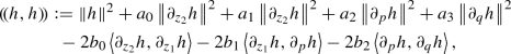
is equivalent to the usual \(H^{1}(\mu )\) inner product, by an inequality similar to (3.5).
-
The operator \(- {\mathcal {L}}\) is coercive in \(H^1_0(\mu )\) endowed with the inner product \(\left( \!\left( \,\cdot \,, \,\cdot \,\right) \!\right) \). More precisely, it holds for any \(h \in H^1_0(\mu )\) that
$$\begin{aligned} - \left( \!\left( h, \mathcal Lh\right) \!\right) \geqslant C(A) \lambda (\mu , \nu , \alpha ) \left( \!\left( h, h\right) \!\right) , \end{aligned}$$where
$$\begin{aligned} \lambda (\mu , \nu , \alpha ) = \min \left( \gamma , \ \frac{1}{\gamma }, \ \frac{\gamma }{\nu ^{4}}, \ \frac{\alpha ^{4} \gamma }{\nu ^{8}}, \ \frac{\alpha ^{2}}{\gamma }, \ \frac{\alpha ^{4}}{\gamma ^{2} \nu ^{2}}\right) . \end{aligned}$$(B.2) -
For any \(h \in L^2_0(\mu )\), it holds
 for \(t \in [0, 1]\), where \(N_h(t)\) is defined by
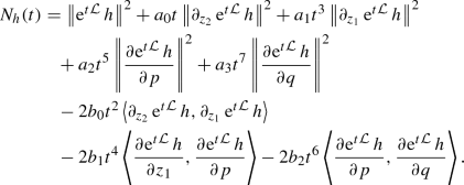

 for
for 
This leads finally to (B.1).
Technical Results Used in Sect. 4.3
In this section, we present technical results that are used in Sect. 4.3. The following estimate is useful in motivating (4.19).
Lemma C.1
Assume that \(c > 0\) is a constant, that h is a smooth function on the torus \({\mathbf {T}}\) and that g is a smooth, everywhere positive function on \({\mathbf {T}}\). Then there exists a unique smooth solution f to the equation

In addition,

Proof
Let \(f_a(q)\) denote the solution to

Since g is smooth and everywhere positive, this equation admits a unique smooth solution on the interval \([-\pi , \pi ]\), by the standard theory of ordinary differential equations. Rewriting the equation for \(f_a\) as

it is clear that
The unique value \(a^*\) for which the function is periodic (namely \(f_{a^*}(\pi ) = a^*\)) is
It is easily checked that all derivatives of \(f_{a^*}\) are also continuous, so that \(f_{a^*} \in C^{\infty }({\mathbf {T}})\).
To obtain the estimate (C.2), we introduce  and note by that, by (C.1),

The term  vanishes at the extrema of r(q), which leads then to (C.2). \(\square \)
We next prove another technical result, which we then employ to show that the leading-order term \({\overline{\phi }}_0\) in the underdamped limit, defined in (4.20), indeed belongs to \(H^1(\mu )\) when V is not constant.
Lemma C.2
If \(q \mapsto V(q)\) is not constant, then there exists \(M > 0\) such that
In particular, \(S_{\nu }(E)\) is bounded below by a positive constant uniformly in \(E\in (E_0,\infty )\).
Proof
Fix \(E > E_0\). We integrate (4.15) over \({\mathbf {T}}\) and use integration by parts for the first term, which gives

We now show that that there exists a positive constant M such that

To this end, notice that  is a decreasing function of E for fixed q, so it is sufficient to show that

Since V is smooth, it holds that  for any q such that \(V(q) = E_0\), so

By using L’Hôpital’s rule, we notice that, for values of q in a neighborhood of any \(q^* \in V^{-1}\{ E_0 \}\) with \(V'(q) \ne 0\),

so L(q) is bounded uniformly from above, implying that (C.6) holds. This concludes the proof because, by (C.5), and recalling that \(s_\nu \geqslant 0\) by (4.16),

and the last integral is positive because V is not constant. \(\square \)
Lemma C.3
If \(q \mapsto V(q)\) is not constant, then the function \({\overline{\phi }}_0\) defined in (4.19) belongs to \(H^1(\mu )\).
Proof
It is easy to see that the function \({\overline{\phi }}_0\) defined in (4.19) belongs to \(L^2(\mu )\). We next consider the distributional derivatives  for \(y \in \{q,p\}\), since derivatives in z vanish: For \(H(q,p) < E_0\), these derivatives vanish; while for \(H(q,p) > E_0\), it holds
  and
and  . Note that all these derivatives belong to \(L^{\infty }_{\mathrm{loc}}({\mathbf {T}}\times {\mathbf {R}}\times {\mathbf {R}})\) in view of the lower bound provided by (C.4). Moreover, \(\left| \nabla {{\overline{\phi }}}_0(q, p, z)\right| \) grows sufficiently slowly as \(|p| \rightarrow \infty \). This allows to conclude that \({\overline{\phi }}_0 \in H^1(\mu )\), as claimed. \(\square \)
Rights and permissions
About this article

Cite this article
Pavliotis, G.A., Stoltz, G. & Vaes, U. Scaling Limits for the Generalized Langevin Equation. J Nonlinear Sci 31, 8 (2021). https://doi.org/10.1007/s00332-020-09671-4
Received:
Accepted:
Published:
DOI: https://doi.org/10.1007/s00332-020-09671-4
Keywords
- Generalized Langevin equation
- Quasi-Markovian models
- Longtime behavior
- Hypocoercivity
- Effective diffusion coefficient
- Overdamped and underdamped limits
- Fourier/Hermite spectral methods