

Abstract
In this study, we investigate a couple of nonlinear fractional differential equations namely, the sine-Gordon and Burgers equations in the sense of Riemann-Liouville fractional derivative. In order to examine exact solutions effectively applicable in relaxation and diffusion problems, crystal defects, solid-state physics, plasma physics, vibration theory, astrophysical fusion plasmas, scalar electrodynamics, etc. we introduce the new generalized  -expansion method. The method is highly effective and a functional mathematical scheme to examine solitary wave solutions to diverse fractional physical models.
Export citation and abstract BibTeX RIS

Original content from this work may be used under the terms of the Creative Commons Attribution 4.0 licence. Any further distribution of this work must maintain attribution to the author(s) and the title of the work, journal citation and DOI.
1. Introduction
The fractional derivatives and integrals is not a new thinking . It has been found that the roots of it were educated over three hundred years ago. In recent decades, considerable efforts have been paid in the fields of NFDEs and draw attention for their frequent appearance in different engineering and scientific arenas, like plasma physics, controlled thermonuclear fusion, solid-state physics, acoustics, diffusive transport, stochastic dynamical system, electrical network, astrophysics, electromagnetic theory, etc. Fractional calculus is used to formulate and interpret different physical models for a continuous transition from relaxation to oscillation phenomena. Therefore, diverse methods have been presented to attain solutions of NFDEs, such as the local fractional Riccati differential equation [1], modified auxiliary equation [2], FRDTM [3], sine-Gordon expansion [4], IBSEF [5],  -expansion [6, 7], modified simple equation [8], Lie symmetry group [9–11], Exp-function [12], exp
 -expansion [13], modified Kudryashov [14] method etc.
Chen and Lin [15] established new exact solutions to the (2 + 1)-dimensional sine-Gordon equation by utilizing generalized tanh-function expansion method. Later, applying the Jacobi elliptic function method, Zhou et al [16] investigated the soliton solutions to the coupled sine-Gordon equation in nonlinear optics. Recently, Hosseini et al [14] determined the new exact solutions to the coupled sine-Gordon equations by applying the modified Kudryashov method. Rawashdeh [3], Yang et al [1] and Cenesiz et al [17] established exact wave solutions to the Burgers-type equation utilizing fractional reduced differential transform, local fractional Riccati differential equation, and first integral methods respectively.
In this article, we investigate the nonlinear space-time fractional sine-Gordon equation (STFSGE) and space-time fractional Burgers equation (STFBE) which have not been studied by using new generalized  -expansion method. The purpose of this analysis is to achieve wide-ranging and typical wave solutions via hyperbolic, trigonometric, rational functions and establish wave profiles.
2. The preliminaries of fractional derivative
In this section, we discuss some definitions of fractional order  namely the Riemann-Liouville, Caputo and conformable fractional derivatives.
Definition 2.1: The Riemann-Liouville fractional derivative of order  is defined as [18]:

where  and
and 
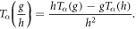
Definition 2.2: The Caputo fractional derivative of order  is defined as [19]:

where  for
for 

 and
and  denote the Caputo fractional derivative and Caputo fractional integral operator respectively.
Definition 2.3: Recently, Khalil et al [20] proposed a new definition of derivative named conformable fractional derivative defined as:

For  and for all
  The characteristics of this definition are given underneath as
  and
and  are differentiable function at
  then
then
-
 for all
-
for all
-
-
-
for all constant functions
- If is differentiable, then


These are the important and useful properties of fractional order derivative. In this study, we will use these properties during establish general and broad-ranging wave solutions.
3. Algorithm of the method
Suppose a general NFDE as:

where  is a polynomial in
 is unspecified function. It consists of the nonlinear terms and fractional-order derivatives. The subscripts represent the partial derivatives.
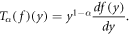
Step 1: Associating the real variables  by a compound variable
  yields

where  is the wave speed, and
  is the fractional order . Utilizing
  by (5), the equation (4) becomes

where  is the polynomial of
  having its derivatives.
Step 2: As per feasibility, integrate (6) several times give arbitrary constants supposed to be zero.
Step 3: We consider the solution structure of equation (6) as:

where  and
and  may separately be zero, but both cannot be zero together,
  for
for  and
and  for
for  and
and  are arbitrary constants. Also,
  is defined as:

where  satisfies the nonlinear ODE:

where  and
and  be the indeterminate.
Step 4: To calculate the balance number  we check the homogeneous balance between the nonlinear highest order exponents and highest order derivatives arising in (6).
Step 5: Substituting (7) and (9) along with (8) into equation (6) having the value of  gained from Step 4, we get a polynomial in
  and
and  Afterword, we assimilate each coefficient of the attained polynomial to zero delivers a set of algebraic equations for
  and
and 
 and
and 
Step 6: The constants  for
for  and
and  for
for 
 and
and  be estimated by calculating the algebraic equations gained in Step 5. As the solution of equation (10) is familiar, substituting
  and
and 
 and
and  into equation (8), we achieve standard and further-reaching wave solutions to the FPDE (4).
Using equation (10) and combining (9), it is reported:
Family 1: If  and
and  then
then

Family 2: If  and
and  then
then
Family 3: If  and
and  then
then

Family 4: If  and
and  then
then

Family 5: If  and
and  then
then

4. Formulation of solutions
In this paragraph, we discuss the applications of the two important models, such as the nonlinear STFSGE and STFBE.
4.1. The space-time fractional sine-Gordon equation
The STFSGE involves sine function and widely used in classical lattice dynamics, the propagation of waves, the extension of biological membrane, the spread of crystal defects, relativistic field theory, etc. Besides, the fractional order  has notable impact in a bridge, a nonlinear beam and other vibration theories. We consider the STFSGE [12]:

where  is fractional order. If
  the equation (15) reduces to the integer-order sine-Gordon equation as:

Applying  equation (15) transforms into the ODE as:

We achieve the balance number  through homogeneous balance technique. Thus

where 


 are constants.
Substituting (18) together with (8) and (9) into (17), the left-hand side is modified to the polynomial in  for
for  and
and  for
for  Picking up the particular coefficient of the reported polynomial and setting them to zero yields a set of equations for
  and
and  Set-1:


where  are free parameters,
  is the wave celerity.
Set-2: 

Set-3: 

Set-4: 

Since  and
and  we obtain the traveling wave solutions after inserting the values in (19) into (18) along with (10) and simplify as (
 and
and  ):
):


where  and
and  is the wave celerity.
The above solutions can be re-written in terms of  -variables as:
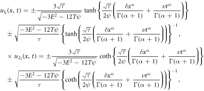
Since  and
and 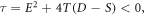 employing (18) accompanying with (11) and calculating from (19), we establish the desired wave solutions (
 and
and ) in terms of spatial and temporal variables in the next:
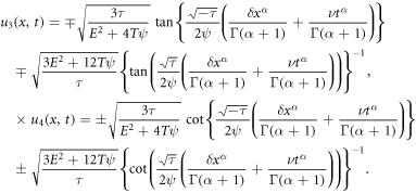
Moreover, since  and
and 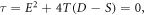 we establish further exact solutions by placing (19) into (18) together with (12) and using the primary wave variable
  and after simplification (
 and
and  ), we derive
Furthermore, since  and
and  we achieve considerable wave solutions in terms of elementary wave variables by setting (19) into (18) along with (13) (
 and
and  ) in the underneath:
Finally, since  and
and  we obtain the trigonometric function solutions by inserting (19) into (18) together with (14) and using the introductory wave variables (
 and
and  ) in the following:
We emphasize that the traveling wave solutions  to
to  be meaningful and resourceful which are applicable in analyzing architectural points of view, vibration theory, applied mathematics, etc.
4.2. The space-time fractional Burgers equation
We consider the STFBE [21]:

where  is physical parameter;
  and
and  are fractional orders. The Burgers equation generally appears in the fields of applied sciences, namely, acoustic waves, ocean engineering, dynamics etc. It interprets the propagation of nonlinear acoustic waves, decay of non-planar shock waves.
If  the equation (23) reduces to the integer-order Burgers equation as:

Applying 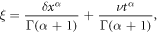 equation (23) converts into the ODE for

where  we integrate it one time, yields

We find the balance number  Therefore, the solution shape is

where  are constants.
In the same procedure, we obtain the new and resourceful sets of solutions as:
Set-1: 

where  are free parameters.


It is expected to ascertain further advanced solution to the fractional Burgers equation for the early mentioned values accumulated in (28)–(31).
For  and
and  placing (28) into solution (27) along with (10) relation to spatial-temporal variables and after simplification, we obtain the wave solutions as (
 and
and  ):
):
where

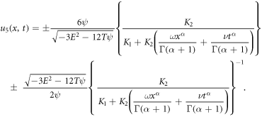
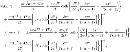
In addition, since  and
and  by means of (28) associating with (11) and from solution (27) subject to the initial variables, we establish the wave solutions in the underneath (
 and
and  ):
):
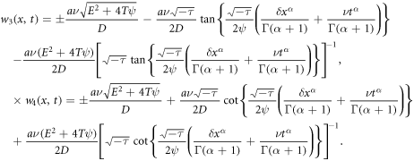
Moreover, inasmuch as  and
and  we bring out more advanced wave solutions about the primary variable
  by introducing (28) into solution (27) together with (12) given in the underneath (
 and
and  ):
):
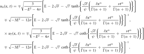
On the other hand, forasmuch as  and
and  we formulate more useful wave solutions by setting (28) into (27) along with (13) concerning basic wave variables as (
 and
and  ):
):

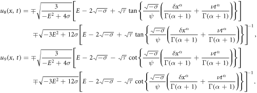
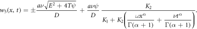
Insofar as  and
and  we obtain the functional exact wave solutions by embedding (28) into (27) together with (14) as (
 and
and  ):
):
The above reported wave solutions from  to
to  be fresh, novel and newly finding resources. The solutions are highly effective and efficient for describing physical systems, such as: modeling, acoustic waves, heat conduction, etc.
5. Graphical representation and physical interpretations
A graph is a crucial tool to depict the physical structures of the phenomena in the sense of real-world applications. The wave solutions are established in terms of trigonometric, hyperbolic and rational function for 
 and
and  respectively. For the values
  and for the fractional order
  the results
  and
and  reflect the kink and singular kink shape wave profile in the interval
 sketched in figures 1 and 2.

Figure 1. Kink shape wave of solution  for
for 
Download figure:
Standard image High-resolution image
Figure 2. Singular kink shape wave of solution  for
for 
Download figure:
Standard image High-resolution imageThe solutions  and
and  provide the singular periodic wave structured maintaining the boundary
 and
and  exhibited in figures 3 and 4 for
  and fractional constant
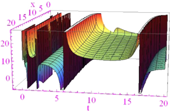
Figure 3. Periodic wave profile of solution  for
for 
Download figure:
Standard image High-resolution image
Figure 4. Periodic wave profile of solution  for
for 
Download figure:
Standard image High-resolution imageThe solution  for
for  and
and  within the range
 and the solutions
  for
for  and
and  within the range
 provide periodic wave profile shown in figures 5 and 6.

Figure 5. Periodic wave profile of solution  for
for 
Download figure:
Standard image High-resolution image
Figure 6. Periodic multi-wave profile of solution  for
for 
Download figure:
Standard image High-resolution imageFor  and
and  within the range
 the solution
  is traced in figure 7. To end, for
  the solutions
  represent exact periodic wave profiles and displayed in figure 8 for
  and
and  within
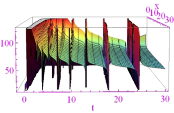
Figure 7. Periodic wave profile of solution  for
for 
Download figure:
Standard image High-resolution image
Figure 8. Exact periodic wave profile of solution  for
for 
Download figure:
Standard image High-resolution image
Remarkably, the fractional-order derivative  leads a significant contribution in modulating the amplitude of the soliton solutions.
6. Conclusion
In this work, we have investigated advanced and functional exact solitary wave solutions of FDEs, namely the sine-Gordon and the Burgers equations. The obtained solutions are kink, singular kink, and exact periodic type wave profiles. The Burgers equation models the nuclear fusion reactor, traffic flow, and steady rainfall on layered field soils. Besides, the sine-Gordon equation is applied for crystal dislocations, the propagation, and creation of ultra-short optical pulses, the motion of rigid pendulum attached to a stretched wire, etc. It also arises in nonlinear optics. The introduced method is effectively applicable for further studies for other nonlinear fractional models.