


Abstract
The hierarchical three-body problem is one of the classical issues of celestial mechanics, but recently it has regained importance due to its applications to new scenarios, like compact objects and exoplanets. In this paper we realize a computational study of this problem using the TIDES software package, which is applied not only to a set of theoretical cases but also to actual stellar systems. The characteristics of the Taylor series integration method, used by TIDES, permit the confirmation of the appearance of the Lidov–Kozai cycles in the case of high mutual inclinations. In addition, a historical review of this problem is included.
Export citation and abstract BibTeX RIS
1. Introduction
Gutzwiller (1998) was correct when he affirmed that the oldest case of the three-body problem is that of the Moon, the Sun, and the Earth. In view of this, with the objective of elaborating a theory concerning the movement of our natural satellite, eminent scientists such as Newton (1687), Euler (1753, 1772), Lagrange (1764, 1873), Laplace (1802), Hansen (1838, 1858, 1863), Delaunay (1858, 1860, 1866), Hill (1877, 1878, 1886, 1890, 1895, 1897, 1899, 1908), Hill & Delaunay (1891), Brown (1896), Poincaré (1900a, 1900b), Brouwer & Rossoni (1960), Brouwer (1962), Hori (1963), Deprit et al. (1970a, 1970b, 1971a, 1971b, 1971c, 1971d), etc., have all dedicated themselves to research about this mathematical and astronomical problem. Their goal has been to ensure that the calculated positions approximate those observed as much as possible. Thus, lunar theory has become one of the most important issues in the field of celestial mechanics.
As an extension of this research, application to the stellar case arose in the first decades of the 20th century and became known as the stellar problem of three bodies, which concerns the study of the movement of three stars Pi (i = 1, 2, 3) with respective masses  (i = 1, 2, 3) that are in a hierarchical configuration in the sense that star P3 is sufficiently separated from the other two stars that we are able to consider perturbed Keplerian movements, such as movement of P3 with respect to the center of masses of P1 and P2 (outer orbit) as well as that of P2 around P1 (inner orbit).
In that case and in agreement with the method of variation of the constants, we then proceed to consider the elements of both orbits as functions of time to be determined, but with the assumption, verified in practice, that in each instant the said orbits can be considered to be Keplerian, with their elements varying from one instant to another. This last issue has the advantage that the integrals and other expressions of the two-body problem can be utilized.
The great difference between this stellar problem and lunar theory is that now the three masses are all of the same order and the eccentricities and the angle formed by the two orbits (the mutual inclination) do not necessarily have small values. On the contrary, according to each case, these parameters can be very different.
Slavenas (1927), using the lunar theory of Hill, began to work with some restrictions, e.g., by taking coplanar movements, Keplerian movements, and the circular outer orbit. Lyttleton (1934) used the equations of Pontécoulant (Brown 1896) and obtained a formulation that permitted the study of the gravitational influence of a third star on the reproduction of eclipses in binaries with application to Algol.
In 1936 and 1937, Brown (1936a, 1936b, 1936c, 1937) developed significant research on the topic, limiting it to detectable terms by means of observation. In his communications, he began to adapt the lunar theory of Delaunay, recognizing the defect that Delaunay considered only small eccentricities and inclinations, which Brown improved in a second paper. In the third part of his work, using the canonical equations of Delaunay, he contributed expressions for the calculation of apse–node terms. Finally, he applied this theory to the ξ-Ursae Majoris system, which, in spite of being a quadruple system, has two of its components so close to each other that, at the first approximation, it may be considered to be a hierarchical triple system. In fact, it is perhaps the best example to use in order to detect orbital perturbations.
Ishida (1949) reviewed the work of Brown and obtained expressions for the calculation of long-period perturbations as well as apse–node terms, applying them to the ζ-Cancri system. Z. Kopal also investigated this problem, and he dedicated one section of his book Close Binary Systems (Kopal 1959) to the perturbations that affected a binary due to interaction with a third body. On the other hand, he also mentioned on page 124 the research made by Hodgkinson, who also followed the work of Brown in the use of the canonical equations of Delaunay. In addition, he developed a complete treatment of short-period perturbations, of special importance in the case of eclipsing systems.
The stellar three-body problem was also studied by Musen (1966). He eliminated short-period terms, applying the averaging method of Krylov & Bogoliubov (1947) to the differential equations of Milankovich (1939), which give the perturbations of the Laplace vectors e and the areal velocity c. Musen commented: "The differential equations for the elements affected only by the long period perturbations can be written as a quasi-linear system. We can solve it either by developing the solutions into a power series in a small parameter or by applying the method of successive approximations." He concluded that for small eccentricities, there are resonances for mutual inclinations of I = 39° and I = 141°. The existence of these critical inclinations was confirmed by Lidov (1961, 1962) and Kozai (1962).
From 1968, R.S. Harrington published various articles on the subject. In the first of those as well as in his dissertation (Harrington 1968a) and in contributions derived from the same (Harrington 1968b, 1969, 1970), he developed the Hamiltonian function in powers of the ratio between the semimajor axes of the inner and outer orbits, which is considered to be a small parameter. Next, he integrated the canonical equations of movement by applying the analytic method of von Zeipel (1916) and obtained, after eliminating the short-period terms (those dependent on true anomalies), two other integrals of movement and demonstrated that the semimajor axes do not experience secular perturbations. In that way, he affirmed that hierarchical triple systems are stable except in cases of high mutual inclination, in which the eccentricity and the inclination itself show very long–period variations (Lidov–Kozai cycles). In his 1969 article, Harrington wrote, "The remaining time averaged problem with only the second order Hamiltonian has one additional integral and can be solved. The motion with the third order Hamiltonian included is more complex, in that there may be additional resonances, and the integral does not exist in all cases."
Soderhjelm (1975) obtained the long-period and apse–node terms from Harrington's work and applied them to the case of eclipsing binaries with the objective of studying the variation of light minima due to the effect of the distant component. The same author (Soderhjelm 1982) increased the long-period terms deduced in his first article to the variables L2 and l2 at the same time that he carried out a thorough numerical study of the secular variations of the eccentricity of the inner orbit in relation to the mutual inclination at an interval of P2/P1. He commented: "The most important property of the motion in a triple system is the (e1−g1)—coupling. There is either a circularity or a librational motion, but in any case, the circularity varies periodically." Another numerical study had been previously published by Standish (1972). Soderhjelm (1984) also studied tidal effects in the stellar three-body problem. Other authors have worked on this same scenario—for example, Kiseleva et al. (1998).
Docobo (1977a) used the method of perturbations of Deprit (1969) in place of that of von Zeipel for the first time. The Deprit method is based on the Lie transformation and its application to the initial canonical system with the objective of obtaining canonical systems that are easier to integrate. This method presents clear advantages with respect to that of von Zeipel such that the old and the new variables are not mixed together. Docobo first considered the outer Keplerian orbit but later extended his study keeping in mind the perturbations in both orbits. In that way, all of the relations between the two orbital planes, the plane of the apparent orbits and the invariable plane, were explicitly obtained (Docobo 1977b, 1977c, 1977d, 1978; Docobo & Prieto 1988; Docobo et al. 1992).
Abad (1984) used the system of polar-nodal, or Hill's, variables, considering the ratio between the semimajor axis of the inner orbit and the distance in the periastron of the outer orbit to be a small parameter. He also used the Deprit method to eliminate the angular variables and transformed the reduced equations into a perturbed harmonic oscillator solved by the asymptotic Krylov–Bogoliubov–Mitropolski method (Krylov & Bogoliubov 1947; Bogoliubov & Mitropolski 1961). Within the same research group, Ling (1989, 1991) and Ling et al. (1995) put into practice the stroboscopic method, which is a semianalytic procedure proposed by C. Lubowe and developed by Roth (1979) for application to the case of an artificial satellite. Among other interesting contributions to the hierarchical three-body problem, we also mention the works of Mazeh & Shaham (1979), Delva & Dvorak (1979), Valtonen & Karttunen (2006), and Krymolowski & Mazeh (1999).
Using the octupole-level secular perturbation equations, Ford et al. (2000) studied the evolution of orbital eccentricities and inclinations over timescales that have long been compared to the orbital periods. Their results can be applied to high-inclination as well as coplanar systems. These authors also took into account triple systems containing a close inner binary, discussing the possible interaction between the classical Newtonian perturbations and the general-relativity precession of the inner orbit.
Several criteria have also been established for the study of the stability of hierarchical triple stellar systems—see, for example, Harrington (1972), Szebehely & Zare (1977), Graziani & Black (1981), Black (1982), Donnison & Mikulskis (1994, 1995), Eggleton & Kiseleva (1995), Kiseleva et al. (1994a, 1994b), Mardling & Aarseth (1999), Orlov & Petrova (2000), and Féjoz & Guardia (2016). Andrade & Docobo (2004) also studied stability, keeping in mind the loss of stellar mass in accordance with the different laws dependent on time and separation (the periastron effect).
From the practical point of view concerning the study and classification of triple stellar systems, it is necessary to highlight the large number of contributions of Tokovinin (1993, 1999, 2004, 2014a, 2014b, 2016a, 2016b), Tokovinin & Smekhov (2002), Sterzik & Tokovinin (2002), and Tokovinin et al. (2006), including the preparation of the Multiple Star Catalog (MSC; Tokovinin 1997), which was recently updated (Tokovinin 2018).
In the 1990s, the discovery of the first exoplanets supposed a recuperation of the hierarchical three-body problem. However, it is important to point out that before that time, publications already existed about planets in binary systems—for example, Harrington (1977), Szebehely (1980), and Dvorak (1984), which proposed studies about the stability of planetary orbits as well as the habitability of said planets. In this sense, a robust line of research exists with a great number of contributions by different authors, such as Dvorak (1986), Rabl & Dvorak (1988), Benest (1987, 1988), Marchal (1990), Dvorak et al. (1989), Mikkola (1997), and Lara et al. (2011).
The secular dynamics in hierarchical three-body systems is considered to be an important research field in many astrophysical contexts (Naoz et al. 2013). In the words of these authors, "In this approximation, the orbits may change shape and orientation, on timescales longer than the orbital timescales, but the semimajor axes are constant. For example, for highly inclined triple systems, the Kozai–Lidov mechanism can produce large amplitude oscillations of the eccentricities and inclinations. At the octupole order, for an eccentric outer orbit, the inner orbit can reach extremely high eccentricities and undergo chaotic flips in orientation."
In the abovementioned paper, Naoz et al. derived the secular evolution equations to the octupole order in Hamiltonian perturbed theory. They also corrected an error in some previous treatments of the problem that implicitly assumed a conservation of the z-component of the angular momentum of the inner orbit. At the same time, they mentioned different scenarios that can be studied apart from the stellar three-body problem, such as the case of asteroids and comets with inclined orbits under the gravitational influence of the Sun and Jupiter, exoplanets, and compact objects. A complete list of references to papers on these last issues can be found in Naoz (2016).
The objective of this research is to apply the Taylor Series Integrator for Differential Equations (TIDES) software to the study of the dynamic evolution of the hierarchical problem of three bodies, taking advantage of the fact that this package, based on the Taylor series method, adjusts the order of these series to achieve a better approximation to the solution with very long integration times and short computational times.
First, we carried out a series of tests of a theoretical type, considering different masses and two different values of the parameter  , a1 and a2 being the semimajor axes of the inner and outer relative orbits and e2 being the eccentricity of the outer orbit. That is to say, a2(1 − e2) is the minimum distance between the centers of mass, C, of the P1 and P2 bodies and the third body P3. We also considered cases in which one of the orbits has direct movement and the other retrograde, with mutual inclinations that are large and small, etc.
Then we applied an algorithm established for two actual cases that correspond to triple stellar systems of the type where the first shows a very low mutual inclination, while, in the second, this inclination is high. The idea was to see how TIDES reproduces, for the long term, the Lidov–Kozai cycles in the eccentricity and inclination of the inner orbit when the mutual inclination is high and at the same time to study the behavior of the argument of the periastron, etc.
In the next sections, first, we present a summary of the characteristics of the TIDES package, which has been used, successfully, in some problems of astrodynamics that require great computational effort. For example, in Barrio et al. (2011a, 2011b) the evolution of a Keplerian orbit was analyzed when there was an uncertainty in the initial conditions. This can be applied to the analysis of the evolution of NEO Earth close approaches. In Dena et al. (2015) the existence of symmetrical periodic orbits around the Moon was studied. These orbits are of great interest from the point of view of lunar exploration. Next, we present the differential equations to be integrated and the flowchart and the algorithm prepared to that effect. Finally, we offer the results obtained and corresponding commentaries on theoretical cases as well as on the selected triple stellar systems.
2. About TIDES
The TIDES numerical integrator (Abad et al. 2011, 2012; Abad & Barrio 2014) allows us to solve first-order ordinary differential equations (ODEs) numerically by using the Taylor series method. This method, for which other packages exist, such as ATOMFT (Corliss & Chang 1982; Chang & Corliss 1994), Cosy Infinity (Berz & Makino 2001), and Taylor (Jorba & Zou 2005), has been successfully used to solve many problems in dynamical systems and astrodynamics as commented above. Some demanding practical applications can be found in Barrio et al. (2011a, 2011b). Among the features of TIDES the following ones are worthy of mention:
- 1.TIDES integrates numerically ODE problems with double or multiple precision (using the MPFR and GMP libraries) by using the Taylor series method in a reasonable computer time.
- 2.The software has been designed to be extremely easy to use: the ODE and its parameters, together with the parameters of the integration, are written in a natural way by means of the Mathematica package MathTIDES, which writes the C (Fortran) code. This code is compiled and linked with the C library libTIDES, thus integrating the ODE.
- 3.The integration is performed with an optimized variable-stepsize and variable-order formulation and extended formulas for variational equations.
- 4.TIDES may detect events of ODEs, i.e., points where a function of the solution of the ODE satisfies an event function, e.g., it becomes zero or reaches an extremum.
- 5.TIDES can handle directly equations that show special sensitivity with respect to initial conditions or parameters, up to any order.
- 6.Automatic differentiation (AD) techniques obtain the derivatives and partial derivatives.
- 7.MathTIDES writes automatically the code for computing partial derivatives of the solution of the ODE with respect to any variable or parameter (using AD and avoiding the use of any variational equation or sensitivity with respect to the parameters).
Now we describe some of the mathematical aspects that constitute the foundations of this software. Let us suppose an initial-value problem represented by the equations

where t0 is the initial instant, x0 is the vector of the initial conditions, and p is a set of m parameters. The solution in a neighborhood of the initial instant can be expressed by means of its Taylor series expansion, which if approximated to the Nth order can be written as follows:

where xk denotes constants that depend on t0 and x0. Replacing the series expansion (2) of x(t) in the differential Equation (1), we obtain on the one hand

and on the other
The coefficient Fk = Fk(x0,...,xk−1) depends on the first k − 1 coefficients of (2).
Combining (3) and (4) we obtain the relationship

This relationship permits us to obtain the terms in each order of the series expansion (3) of the solution of the problem.
The procedure used in TIDES for the obtainment of (3) requires the application of AD techniques based on the algebraic manipulation of power series that can be found in Abad et al. (2011).
The use of the series (3) to calculate the numerical value of the solution in any point t requires us to take into account two important subjects: first the determination of the order N for which the error of a series of this order is below a certain value and second the convergence radius of the series, i.e., the value h for which the series is absolutely convergent for ∣t − t0∣ < h. This value yields the values of t for which it is possible to evaluate the value of x(t) by using its power series expansion. If point t belongs outside of the convergence radius of the series, a new initial value must be obtained by means of t0 = t0 + h, x0 = x(t0 + h), and the AD process must be applied again to obtain (3) until t is located within its radius of convergence. The numerical details of this procedure are also detailed in Abad et al. (2011).
3. The Proposed Algorithm
The Newtonian equations of the three-body problem formulated in Jacobian coordinates were integrated using the TIDES package.
Starting from the orbital elements of the two orbits (inner and outer), the position and velocity vectors, ri(0) and  (0) with i = 1, 2, were calculated using an application in Python, in a chosen initial instant. These initial values were introduced in TIDES to perform integrations of the following equations (Abad 2012) describing the two mentioned orbits:
where  ,
,  , and
, and  are the masses of the three bodies P1, P2, and P3. According to the definition of the center of mass of the bodies P1 and P2, C, one has

where r1 is the position vector of P2 with respect to P1 and r2 is the position vector of P3 with respect to the center of mass of P1 and P2 (see Figure 1).

Figure 1. Graphic representation of the positions of the three bodies.
Download figure:
Standard image High-resolution imageAt each integration, TIDES generates a file in plain-text format that, for each instant of time ti, provides the position and velocity vectors ri(j) and  with i = 1, 2, and j = 1, ..., S, where S denotes the integration steps. This file is processed by the Python application, which, through a series of calculations, generates the osculating orbital elements.
The flowchart of the application in Python and TIDES is shown in Figure 2.
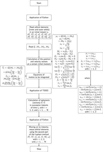
Figure 2. Flowchart of the algorithm.
Download figure:
Standard image High-resolution imageBefore applying our algorithm to real stellar systems, we included the application of TIDES to three groups of theoretical cases. In group A, we varied the mutual distance considering two values for the parameter  , 0.1 and 0.15, and also considered that the three masses were equal and that the third body P3 had a mass that was three times that of each of the other two bodies.
In the second group, B, we focused on the mutual inclination Im of both orbits, which was calculated using the expression (Docobo 1977a; Docobo et al. 2016)

We considered cases in which Im was very elevated and others where Im was very low.
Lastly, in relation to the direction of the motion of the two orbits, we selected two situations with orbits co-revolving and orbits having contrary directions with the goal of studying the behavior of the angle ω (group C).
4. Theoretical Cases
In this section we present the 12 theoretical cases previously mentioned, which will be used as a test to the developed algorithm. Tables 1, 2, and 3 contain the orbital elements and masses considered for each case, given in the format used for visual binaries.
Table 1. Orbital Elements and Masses for the Group A Cases
| P (years) | T (years) | e | a ('') | I (°) | Ω (°) | ω (°) | = 
|
||
|---|---|---|---|---|---|---|---|---|---|
| A1 | outer orbit | 302.4 | 0. | 0.4 | 11.1 | 20. | 60. | 80. | 0.15 |
| A1 | inner orbit | 10. | 100. | 0.2 | 1. | 40. | 120. | 100. | |
Masses:  = 1 = 1   = 1 = 1   = 1 = 1 
|
|||||||||
| A2 | outer orbit | 555.6 | 0. | 0.4 | 16.7 | 20. | 60. | 80. | 0.10 |
| A2 | inner orbit | 10. | 100. | 0.2 | 1. | 40. | 120. | 100. | |
Masses:  = 1 = 1   = 1 = 1   = 1 = 1 
|
|||||||||
| A3 | outer orbit | 234.2 | 0. | 0.4 | 11.1 | 20. | 60. | 80. | 0.15 |
| A3 | inner orbit | 10. | 100. | 0.2 | 1. | 40. | 120. | 100. | |
Masses:  = 1 = 1   = 1 = 1   = 3 = 3 
|
|||||||||
| A4 | outer orbit | 430.3 | 0. | 0.4 | 16.7 | 20. | 60. | 80. | 0.10 |
| A4 | inner orbit | 10. | 100. | 0.2 | 1. | 40. | 120. | 100. | |
Masses:  = 1 = 1   = 1 = 1   = 3 = 3 
|
|||||||||
Download table as: ASCIITypeset image
Table 2. Orbital Elements and Masses for the Group B Cases
| P (years) | T (years) | e | a ('') | I (°) | Ω (°) | ω (°) | = 
|
||
|---|---|---|---|---|---|---|---|---|---|
| B1 | outer orbit | 555.6 | 0. | 0.4 | 16.7 | 20. | 60. | 80. | 0.10 |
| B1 | inner orbit | 10. | 100. | 0.2 | 1. | 90. | 120. | 100. | |
Masses:  = 1 = 1   = 1 = 1   = 1 = 1  Im = 80 Im = 80 2 2 |
|||||||||
| B2 | outer orbit | 555.6 | 0. | 0.4 | 16.7 | 45. | 60. | 80. | 0.10 |
| B2 | inner orbit | 10. | 100. | 0.2 | 1. | 55. | 90. | 100. | |
Masses:  = 1 = 1   = 1 = 1   = 1 = 1  Im = 249 Im = 249 |
|||||||||
| B3 | outer orbit | 430.3 | 0. | 0.4 | 16.7 | 20. | 60. | 80. | 0.10 |
| B3 | inner orbit | 10. | 100. | 0.2 | 1. | 90. | 120. | 100. | |
Masses:  = 1 = 1   = 1 = 1   = 3 = 3  Im = 802 Im = 802 |
|||||||||
| B4 | outer orbit | 430.3 | 0. | 0.4 | 16.7 | 45. | 60. | 80. | 0.10 |
| B4 | inner orbit | 10. | 100. | 0.2 | 1. | 55. | 90. | 100. | |
Masses:  = 1 = 1   = 1 = 1   = 3 = 3  Im = 249 Im = 249 |
|||||||||
Download table as: ASCIITypeset image
Table 3. Orbital Elements and Masses for the Group C Cases
| P (years) | T (years) | e | a ('') | I (°) | Ω (°) | ω (°) | = 
|
||
|---|---|---|---|---|---|---|---|---|---|
| C1 | outer orbit | 555.6 | 0. | 0.4 | 16.7 | 25. | 60. | 80. | 0.10 |
| C1 | inner orbit | 10. | 100. | 0.2 | 1. | 85. | 120. | 100. | |
Masses:  = 1 = 1   = 1 = 1   = 1 = 1  Im = 7317 Im = 7317 |
|||||||||
| C2 | outer orbit | 555.6 | 0. | 0.4 | 16.7 | 25. | 60. | 80. | 0.10 |
| C2 | inner orbit | 10. | 100. | 0.2 | 1. | 120. | 120. | 100. | |
Masses:  = 1 = 1   = 1 = 1   = 1 = 1  Im = 10567 Im = 10567 |
|||||||||
| C3 | outer orbit | 430.3 | 0. | 0.4 | 16.7 | 60. | 80. | 80. | 0.10 |
| C3 | inner orbit | 10. | 100. | 0.2 | 1. | 85. | 60. | 100. | |
Masses:  = 1 = 1   = 1 = 1   = 3 = 3  Im = 3132 Im = 3132 |
|||||||||
| C4 | outer orbit | 430.3 | 0. | 0.4 | 16.7 | 110. | 90. | 80. | 0.10 |
| C4 | inner orbit | 10. | 100. | 0.2 | 1. | 85. | 70. | 100. | |
Masses:  = 1 = 1   = 1 = 1   = 3 = 3  Im = 3180 Im = 3180 |
|||||||||
Download table as: ASCIITypeset image
The evolution in a time interval that corresponds to 1000 times the period of the outer orbit, P2, for each of the orbital elements of both orbits in the 12 cases studied (168 graphs) is included in the online version of this article:
- (A)By mutual distances and masses
- (B)By mutual inclination
- (C)By direction of movement
We begin with cases A1 and A2 of section A. In both cases, the angle of the node of the inner orbit makes a complete revolution in direct motion, but in the case of A1, the revolution is completed in 90,000 years, while in case A2, it occurs three times as rapidly (see Figure 3). Something similar happens with the angle of the node of the outer orbit, but in this case, this element is in libration (see Figure 4).
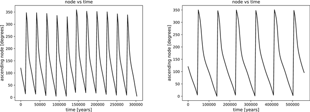
Figure 3. Perturbation in the angle of the node of the inner orbits in cases A1 and A2.
Download figure:
Standard image High-resolution image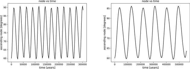
Figure 4. Perturbation in the angle of the node of the outer orbits in cases A1 and A2.
Download figure:
Standard image High-resolution imageChanging cases A1 and A2 for A3 and A4, we see the differences clearly increase given that the perturbing body has more mass (see Figure 5).

Figure 5. Comparison of the angles of the nodes of the inner and outer orbits in cases A3 (first two figures above) and A4 (last two figures below).
Download figure:
Standard image High-resolution imageStudying the evolution of the two inclinations (the inner and outer orbits) for cases A1 and A3 (with the same value), one can see, as one would expect, that the variations in those orbital elements occur more rapidly in A3 given that the P3 body has, in this case, triple the mass of that in the A1 situation. Therefore, inclination I1 varies in case A1 between 50° and less than 10° in approximately 25,000 years. In case A3, it occurs in some 10,000 years and not exactly in the same limits (see Figure 6). For inclination I2, the evolution of the elements occurs in a manner similar to that seen in Figure 7.
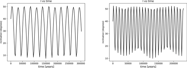
Figure 6. Comparison of the inclination of the inner orbits in cases A1 and A3.
Download figure:
Standard image High-resolution image
Figure 7. Comparison of the inclination of the outer orbits in cases A1 and A3.
Download figure:
Standard image High-resolution imageIn relation to the e1 and e2 eccentricities, we have also carried out a comparison between cases A2 and A4. Figure 8 confirms the expected logic, which is that the perturbations are greater than those in case A4.
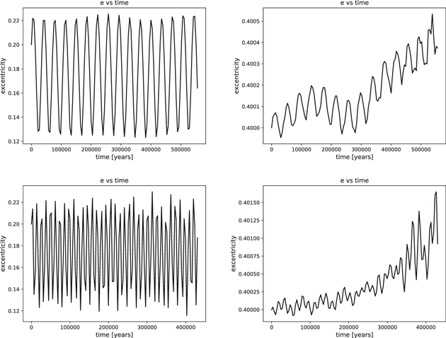
Figure 8. Comparison of the eccentricity of the inner and outer orbits in cases A2 (first two figures above) and A4 (last two figures below).
Download figure:
Standard image High-resolution imageMoving to block B, in which we take different values of the mutual inclination of the orbits, we find the behavior of the elements e1, e2, I1, I2, Ω1, Ω2, ω1, and ω2 to be of maximum interest.
In cases B1 and B3, the mutual inclination is high (802), whereas in B2 and B4 it is low (249). It is precisely this parameter that is going to be decisive in the type of evolution of each element. In effect, considering the B1 case, with the mutual inclination between 39° and 141°, the mechanism of Lidov–Kozai is produced in such a way that, in the inner orbit, the eccentricity e1 is affected by strong perturbations that make it oscillate until it reaches values close to one.
For the part of the inclination of the inner orbit, I1, ample oscillations are also presented that cause the initial direct orbit to move in retrograde motion and vice versa, while the argument of the periastron, ω1, is in libration (see Figure 9).
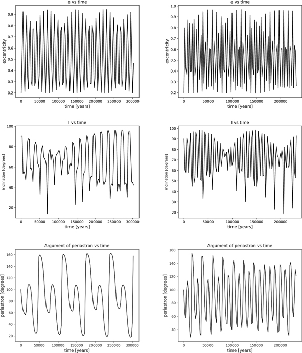
Figure 9. Comparison of the eccentricity, inclination, and argument of the periastron of the inner orbits in cases B1 and B3.
Download figure:
Standard image High-resolution imageIn case B2, the same does not occur, where the behavior of e1 and I1 is merely periodic with the e1 eccentricity oscillating between 0.175 and 0.227 and the I1 inclination between 24° and 68° and now it is the ω1 argument of the periastron that is in circularization, passing from 0° to 360° in approximately 600,000 years (see Figure 10).

Figure 10. Comparison of the eccentricity, inclination, and argument of the periastron of the inner orbit in case B2.
Download figure:
Standard image High-resolution imageWith respect to the outer orbit, in case B1, the eccentricity e2 has a periodic variation of low amplitude, while in the inclination I2, the periodic behavior is observed to have variable amplitude. In any case, the value oscillates between 16° and 37° in 300,000 years. Regarding the argument of the periastron, a secular evolution is present with a periodic component superimposed, but ω2 makes a complete revolution of 0°–360° in approximately 225,000 years (see Figure 11).
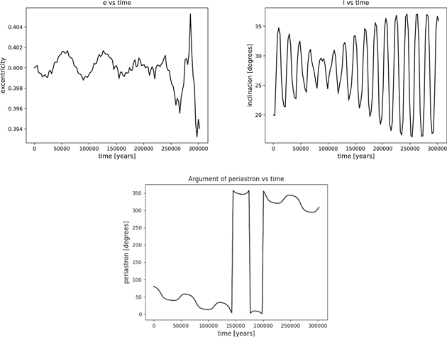
Figure 11. Comparison of the eccentricity, inclination, and argument of the periastron of the outer orbit in case B1.
Download figure:
Standard image High-resolution imageIn case B2, e2 demonstrates an extremely small variation, increasing by only two thousandths in more than 500,000 years. The argument of the periastron, ω2, increases secularly from 0° to 360° in almost 600,000 years (see Figure 12).

Figure 12. Comparison of the eccentricity and argument of the periastron of the outer orbit in case B2.
Download figure:
Standard image High-resolution imageFinally, in scenario C, we consider orbits with the same (C1 and C3) and opposite (C2 and C4) directions of movement. Cases C1 and C2 show a high mutual inclination, while in C3 and C4, the mutual inclination is low. We want to know if the fact that these are systems with contrary directions of movement may influence the Lidov–Kozai cycles. Our comparisons indicate that the answer is no. In cases C1 and C2, we should expect those cycles due to the high mutual inclination, but we should not expect so in the other two cases. Selecting the C1 and C2 cases, we see that in the first, with respect to the eccentricity of the inner orbit (e1) there are strong oscillations that reach values superior to 0.9 as in cases B1 and B3. However, the fact that the orbital movements occur in opposite directions does not change this behavior as can be seen in C2.
The same occurs with the inclination I1 such that in both cases there are successive changes in the quadrant and the argument of the periastron, ω1, which maintains the libration in both C1 and C2 (see Figure 13).
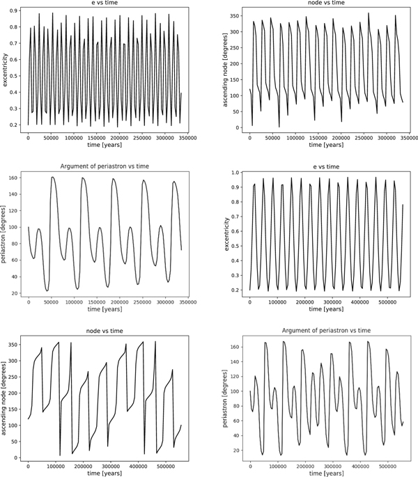
Figure 13. Comparison of the eccentricity, inclination, and argument of the periastron of the inner orbits in cases C1 (first three figures) and C2 (last three figures).
Download figure:
Standard image High-resolution imageIn the cases of low mutual inclination, the fact that the two orbits have contrary directions of movement does not affect the behavior shown in the case of B. For example, in case C4, with low mutual inclination and orbits in opposite directions, the eccentricity (e2) and the inclination (I2) maintain the periodic character of low amplitude in which ω2 demonstrates circularization (see Figure 14).

Figure 14. Comparison of the eccentricity, inclination, and argument of the periastron of the outer orbit in case C4.
Download figure:
Standard image High-resolution image5. Application to Stellar Systems
The algorithm developed, and tested in the theoretical cases, has been applied to two hierarchical triple stellar systems: HD 200580 and HD 213052. The orbital elements of these systems (outer and inner orbits) with their corresponding errors are shown in Table 4. In it, the first column identifies each subsystem by the HD number and, in the line below, by the discover code and component designations. The following columns indicate the orbital period P, the epoch of the periastron passage T, the eccentricity e, the semimajor axis a, the inclination I, the node Ω, and the argument of the periastron ω.
Table 4. Orbital Elements
| HD/System | P | T | e | a | I | Ω | ω |
|---|---|---|---|---|---|---|---|
| Other Designation | (year) | (year) | ('') | (°) | (°) | (°) | |
| Reference | |||||||
| 200580 / outer | 19.205 | 2006.259 | 0.1743 | 0.2195 | 65.1 | 102.8 | 17.6 |
| WSI 6AB | ± 0.080 | ± 3.60 | ± 0.0083 | ± 0.0013 | ± 1.0 | ± 0.5 | ± 2.6 |
| Tokovinin & Latham (2017) | |||||||
| 200580 / inner | 1.03483 | 2014.6223 | 0.0934 | 0.0284 | 68.6 | 97.3 | 124.9 |
| DSG 6Aa,Ab | ± 0.00008 | ± 0.0089 | ± 0.0040 | ± 13.7 | ± 12.5 | ± 3.1 | |
| Tokovinin & Latham (2017) | |||||||
| 213052 / outer | 540 | 1981.50 | 0.419 | 3.496 | 142.0 | 131.3 | 269.3 |
| STF 2909AB | ± 15 | ± 0.58 | ± 0.011 | ± 0.046 | ± 0.4 | ± 0.8 | ± 1.7 |
| Tokovinin (2016b) | |||||||
| 213052 / inner | 25.95 | 206.52 | 0.872 | 0.110 | 11.8 | 293.7 | 100.9 |
| EBE 1Aa,Ab | ± 0.048 | ± 0.13 | ± 0.006 | Fixed | ± 6.7 | ± 74 | ± 73 |
| Tokovinin (2016b) | |||||||
Download table as: ASCIITypeset image
5.1. HD 200508
This is a spectroscopic–interferometric system (both the inner AaAb pair and the outer AB) studied by Tokovinin & Latham (2017). The outer WSI 6AB system was resolved by Mason et al. (2001), and the inner DSG 6AaAb system by Horch et al. (2012). In 2002, Latham et al. calculated the spectroscopic orbit (SB1) of the closed binary (Latham et al. 2002).
The combined spectrum is considered as F9V in the SIMBAD database (Wenger et al. 2000), although some measurements suggest it may be F7V or F8V. The magnitudes listed in the ORB6 catalog (Hartkopf et al. 2001) are 7.5–9.5 for AB and 7.6–9.1 for AaAb (the latter is based on the observations of E. Horch). Nevertheless, Tokovinin & Latham considered that the difference of magnitudes of the inner system should be at least 4.1 because it was not resolved by the CHIRON spectrometer.
The measurements by Horch were obtained close to the diffraction limit of the telescope, and for that reason, it is possible that the difference of magnitude is underestimated. As such, Tokovinin & Latham gave magnitudes of 7.46, 12.5, and 9.62 with 1.15, 0.56, and 0.67 as the respective masses for the Aa, Ab, and B components. With these values and keeping in mind the Gaia parallax (Gaia Collaboration et al. 2018), we have resulting absolute magnitudes of 4.15, 9.20, and 6.32, which correspond to the F8V, M1V, and K1V spectral types, respectively. It is a metal-poor system, with [Fe/H] = −0.51 in the Geneva–Copenhagen Catalog (Holmberg et al. 2009) and values ranging from −0.43 to −0.80 in the abundance measurements listed in SIMBAD. The estimated age is between 7.2 and 8.9 Gyr in the catalog, which suggests that the system is stable.
This system has a low mutual inclination (Im = 615), so the Lidov–Kozai cycles are not expected. In this case the integrations were made over only 1000 times the orbital period of the outer orbit (19,000 years approximately). The evolution of the orbital elements of both the inner and the outer orbits (Tokovinin & Latham 2017) is represented in the graphs of Figures 15 and 16. Perturbations in T and a are merely periodic, e.g., a1 varies between 0 02834 and 002850, and a2 between 02193 and 02202.
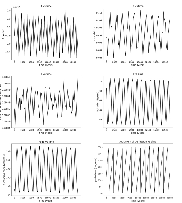
Figure 15. Evolution of the orbital elements of the inner orbit for the HD 200580 system.
Download figure:
Standard image High-resolution image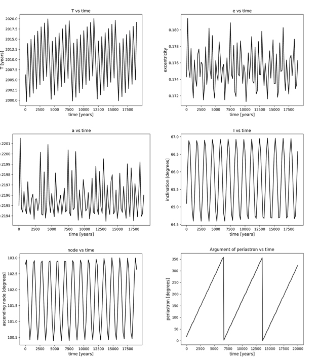
Figure 16. Evolution of the orbital elements of the outer orbit for the HD 200580 system.
Download figure:
Standard image High-resolution imageAs expected, with such a low mutual inclination, the eccentricity and the inclination of the inner orbit, e1 and I1, show periodic perturbations of minimal amplitude: e1 varies between 0.080 and 0.110, while I1 varies between 61° and 70°. The angle of the node is in libration from 96° to 107°, while ω1 circularizes, making a complete revolution in 1250 years.
The perturbations in the outer orbit are smaller, being purely periodic in e2, I2, and Ω2 but secular in ω2, which goes from 0° to 360° in 7500 years.
5.2. HD 213052 (Zeta Aquarii)
In calculating the orbit of the AB binary, Strand (1942) considered the possible existence of a third body. Later orbits calculated by Rabe (1954), Franz (1958), Harrington (1968c), Costa & Docobo (1982), Heintz (1984), Olevic & Cvetkovic (2004), and Scardia et al. (2010) with more visual as well as photographic observations confirmed this fact. The AaAb components of star A were resolved in 1978.96 using speckle interferometry (Ebersberger & Weigelt 1979). Later, Tokovinin (2016b) considered that measurement improbable due to the then-established difference of magnitude between the Aa and Ab components, Δm = 6.3. Therefore, he proposed the following values: Aa, 4.30; Ab, 10.60; and B, 4.51, with corresponding masses of 1.4, 0.6, and 1.4. Tokovinin considered Aa and B to be practically equal evolved stars (spectral type F2IV–V), while Ab could be a main-sequence dwarf. This idea as well as the fact that the mutual inclination is high suggests the possibility that the Ab component was captured after the formation of the system.
Zeta Aquarii had been observed by W. Herschel in 1779, although a previous measurement was listed in a catalog by Mayer in 1784 (Tokovinin 2016b). Gaia (Gaia Collaboration et al. 2018) assigned the parallaxes of AaAb (003451) and B (003425), while Hipparcos (van Leeuwen 2007) measured the parallax of the AB system (003550). Recently, Izmailov (2019) calculated new orbits for this well-known multiple system.
This case is completely different from the previous one in that now the orbits calculated by Tokovinin are more eccentric, especially the inner one. The mutual inclination is also high. However, there are no precise radial velocities (RVs) to be able to determine the nodes, so two values of the mutual inclination are possible. For Ω1 = 1137 and Ω2 = 1313 or Ω1 = 2937 and Ω2 = 3113, we have Im = 1306, but for Ω1 = 1137 and Ω2 = 3113 or Ω1 = 2937 and Ω2 = 1313, we deduce Im = 1531. In the first two cases, because Im < 141°, in accordance with the Lidov–Kozai limits, and in view of the results of the theoretical cases previously studied, we can expect ample variations in e1 and I1, while ω1 should be in libration. The first of these two is what we have considered. If Im = 1531, the Lidov–Kozai mechanism is not expected. RV observations are fundamental to determining the precise nodes.
The evolution of the elements in both the inner and the outer orbits (Tokovinin 2016b) has been calculated in a temporal interval of 500,000 years, close to 1000 times the period of the outer orbit, and it is what can be seen in Figures 17 and 18.
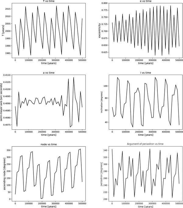
Figure 17. Variation of the orbital elements of the inner orbit for the HD 213052 system over an integration of 500,000 years.
Download figure:
Standard image High-resolution image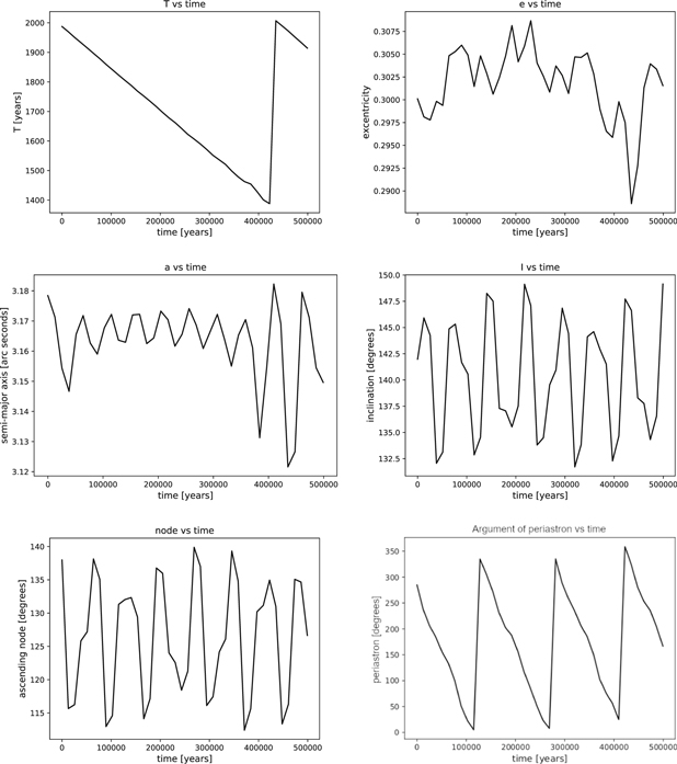
Figure 18. Variation of the orbital elements of the outer orbit for the HD 213052 system over an integration of 500,000 years.
Download figure:
Standard image High-resolution imageWe also have carried out a very long–term integration (5 million years) in order to confirm the tendencies, which indeed occurred (see Figures 19 and 20).
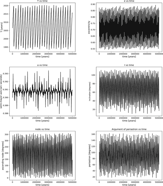
Figure 19. Variation of the orbital elements of the inner orbit for the HD 213052 system over an integration of 5,000,000 years.
Download figure:
Standard image High-resolution image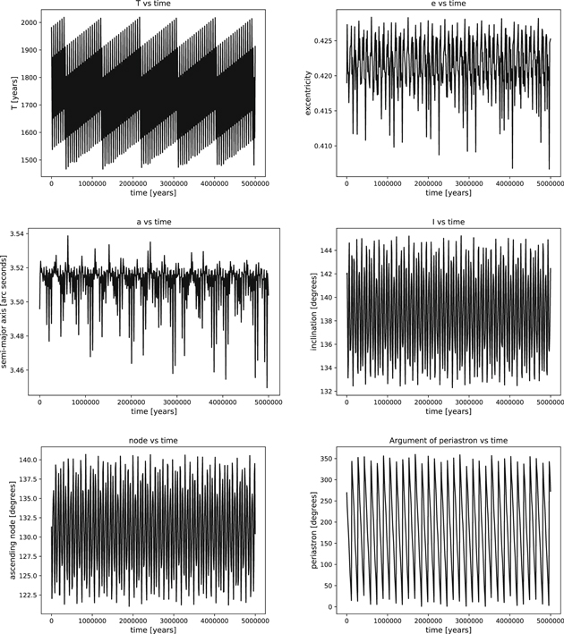
Figure 20. Variation of the orbital elements of the outer orbit for the HD 213052 system over an integration of 5,000,000 years.
Download figure:
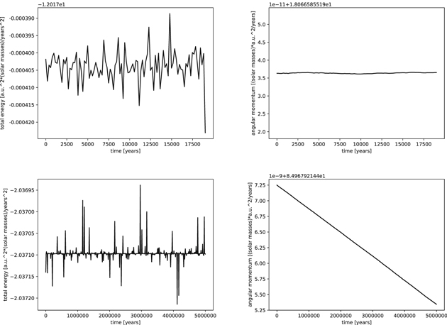
Standard image High-resolution imageIn all of the studied cases, both the angular momentum and the integral of the energy were conserved. We include the corresponding graphs for the two stellar systems considered (see Figure 21).
Figure 21. Evolution of the energy and the angular momentum for HD 200580 and HD 213052.
Download figure:
Standard image High-resolution image
6. Conclusions
In recent years, the hierarchical three-body problem has acquired new relevance given the possible applications to new scenarios such as planetary systems, compact bodies, etc. Taking advantage of this fact, we have carried out a theoretical–practical study of the problem, beginning with a historical review of the different approximations that have yielded the same results. Moreover, we have used the power and versatility of the TIDES package in order to integrate different cases, theoretical as well as practical, in which the effects of different configurations on the results were studied.
We have demonstrated the appearance of the cycles of inclination and eccentricity predicted by Lidov–Kozai without the necessity to use very long integration times. In these cycles, we have confirmed the influence of the mutual inclination between the orbits, with perturbations appearing for inclinations between 39° and 141°.
However, we have rejected the hypothesis that those elements are affected significantly by the direction of orbital movements, due to the fact that systems with co-revolving orbits and those with orbits in opposite directions show the same behavior.
Finally, we have conducted a study of two actual systems, HD 200508, with low mutual inclination, and HD 213052, with an inclination within the limits established by Lidov–Kozai. In both cases, the behavior predicted by the theory was confirmed. In the second case, significant perturbations in the inclination and the eccentricity of the inner orbit appeared, which did not occur in the first case.
The study of the hierarchical problem of three or more bodies is very important in stellar astronomy. The physical and dynamical properties of the components provide information that is associated with the formation and evolution of these systems, including possible captures as occurs in the case of the second system reported in this article. In addition, medium- and long-term tracking of those orbits is fundamental in order to not only assess their stability but also understand the influence that they have on the exoplanets of these systems.
In agreement with the previously mentioned Lidov–Kozai mechanism, high inclinations between the two orbits of a triple stellar system give place, in the medium and long term, to dramatic changes in the inclination and eccentricity of the inner orbit with consequent instability produced in the orbits of planetary subcomponents. These high inclinations may also effect the expulsion of planets from their original systems, which may explain a percentage of unbound exoplanets, particularly those in the lower range of mass. All of the aforesaid may have special influence on the habitability of those planets and their possible exosatellites.
In the present article, we have considered two triple-star systems as examples. It is clear that the theory presented here may be applied to all other systems in which the inner and outer orbits have been well established, which is a powerful reason to continue to obtain high-precision observations of these systems. Regarding this matter, we point out the relevance of contributions such as the MSC of Andrei Tokovinin.
J.A.D., L.P., and P.P.C.'s work was supported by the Spanish Ministerio de Economía, Industria y Competitividad under project AYA-2016-80938-P (AEI/FEDER, UE). A.A.'s work was partially supported by the Spanish Ministerio de Economía, Industria y Competitividad, project no. ESP2017-87113-R (AEI/FEDER, UE), and by the Aragón Government and the European Social Fund (group E24 17R).