2.1 The CESM 1.0.5

The Community Earth System Model (CESM; Hurrell et al., 2013) version 1 is a fully coupled atmosphere–land–ice–ocean general circulation model (GCM) that was developed at the National Center for Atmospheric Research (NCAR) in Boulder, Colorado. For use in palaeoclimate modelling, version 1.0.5 of the CESM is a suitable choice motivated by a trade-off between increasing model complexity and computational cost. This version of the CESM is equivalent to the latest version of the Community Climate System Model (CCSM4; Blackmon et al., 2001; Gent et al., 2011). In the configuration used here, the horizontal resolution of both the atmosphere and ocean is doubled compared to that of Herold et al. (2014), while that of the atmosphere is about 50 % higher than in Hutchinson et al. (2018), with comparable ocean grids.

The atmospheric component of the CESM is the Community Atmosphere Model (CAM4; Neale et al., 2013), which uses a finite-volume grid at a nominal resolution of 2^∘ (2.5^∘ × 1.9^∘) and 26 vertical levels with a hybrid sigma vertical coordinate extending upward to 2 hPa. In this configuration, the model has a reported a warming response of 3.13 ^∘C to a doubling of CO₂ starting from pre-industrial conditions (compared to ∼2.5 ^∘C in CCSM3; Bitz et al., 2012; Kiehl et al., 2006).

The physical, chemical, and biological processes taking place on land are represented in the Community Land Model (CLM4; Oleson et al., 2010; Lawrence et al., 2011). A static rather than dynamic vegetation model is used here to avoid runaway feedback effects, which can become an issue, especially in warm greenhouse climates (e.g. dieback of vegetation at low latitudes; Loptson et al., 2014; Herold et al., 2014). The considered biomes are translated into fractions of the corresponding CLM4 plant functional types (PFTs), from which a set of monthly forcing files is finally used in the model. Freshwater runoff is treated by a simple river-routing scheme, in which all runoff is transported to one of the surrounding eight model grid cells until the ocean is reached. The direction is determined by the local topography gradient and manually adjusted where the runoff scheme would otherwise form closed loops.

The sea ice component consists of the Los Alamos National Laboratory (LANL) Community Ice Code version 4 (CICE4; Hunke and Lipscomb, 2004). For simplicity, sea ice only forms when the sea surface cools down to −1.8 ^∘C, after which its dynamical behaviour (e.g. melt and advection) is specifically treated by the model.

The CESM1 uses the LANL Parallel Ocean Program version 2 (POP2; Smith et al., 2010) for the ocean model component. The standard configuration is applied here, with a nominal 1^∘ (1.25^∘ × 0.9^∘) horizontal resolution on a curvilinear grid placing the northern pole over Greenland. The POP2 model is set up with 60 layers of varying thickness between 10 m near the surface and 250 m at greater depth. Horizontal viscosity is considered anisotropic (Smith and McWilliams, 2003) and horizontal tracer diffusion follows the parameterisation of Gent and Mcwilliams (1990). The model further uses the K-profile parameterisation (KPP) scheme to determine vertical mixing coefficients (Large et al., 1994). More information and discussion on the ocean model physics and parameterisations can be found in Danabasoglu et al. (2008, 2012).

2.2 Model experiments

To allow comparisons of various climatic features between Eocene and pre-industrial conditions within a similar framework, a pre-industrial reference run with the same version of the CESM is performed (using the geography shown in Fig. 1b, e, f). Since the atmospheric component used here consists of the CAM4 at a nominal 2^∘ horizontal resolution, this reference is similar to the 2^∘ 1850 control of Gent et al. (2011). The solar constant in the simulation is 1361.27 W m⁻², and the atmospheric levels of CO₂ and CH₄ are 280 ppm and 671 ppb, respectively (i.e. pre-industrial carbon; PIC). Astronomical orbital parameters are set to their present-day configurations: eccentricity 0.0167, obliquity 23.44^∘, and precession placing the aphelion in Northern Hemisphere summer. Both vegetation and atmospheric aerosols are kept fixed at their respective pre-industrial distributions (Fig. S1), meaning that all anthropogenic influences apart from land cover changes are disregarded. Overflow and tidal mixing parameterisations are switched off for a better comparison to the Eocene cases. Background vertical diffusivity is a constant 0.17 cm² s⁻¹ nearly everywhere, increasing to 0.3 cm² s⁻¹ around 30^∘ N or S and 1 cm² s⁻¹ in the Banda Sea, following Jochum (2009).

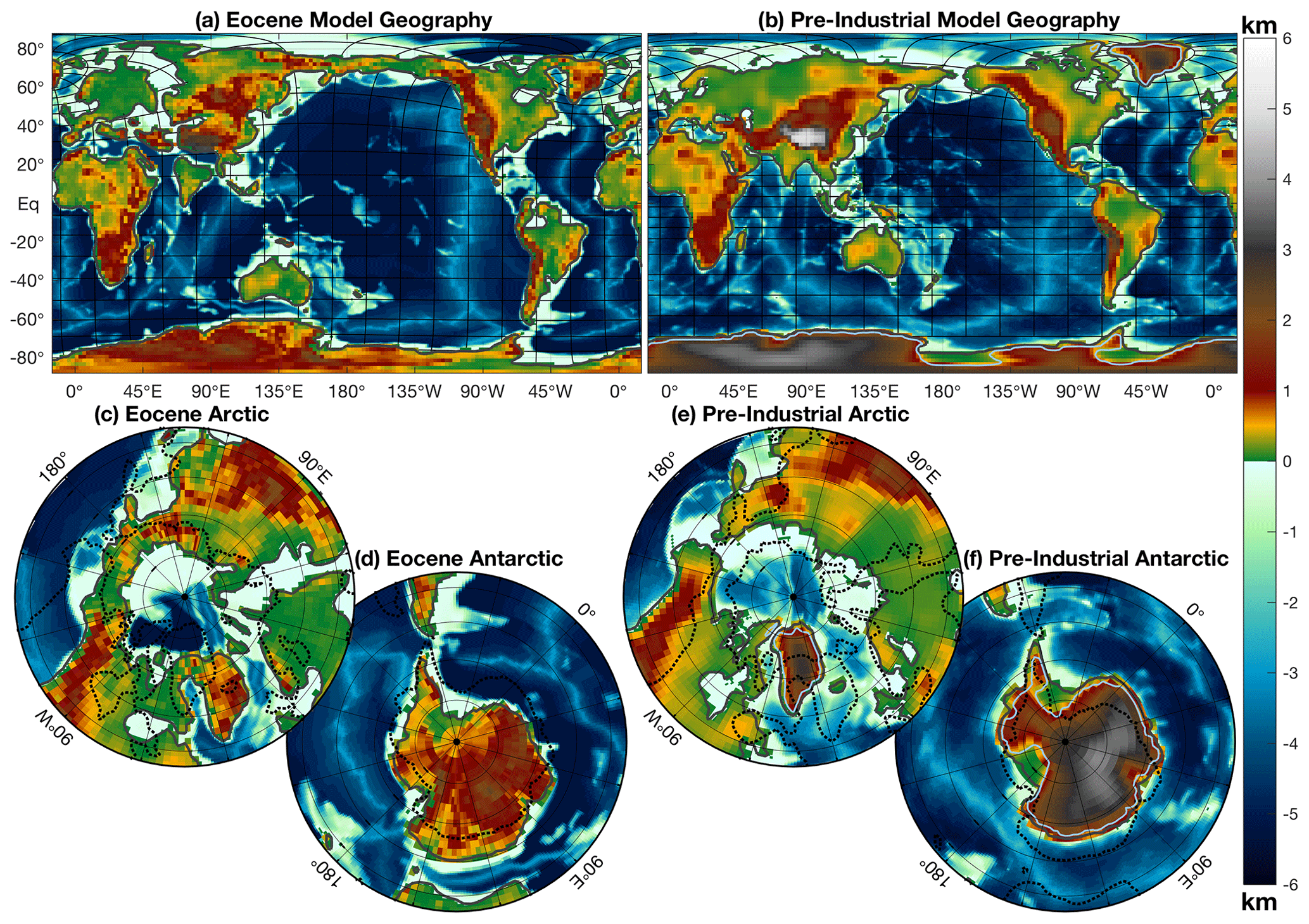
Figure 1Topography (atmosphere) and bathymetry (ocean) grid used in the model simulations for the (a) 38 Ma Eocene cases and (b) pre-industrial reference. Black lines are drawn every 20 model grid boxes for the ocean, and the thick grey line shows the coastlines defined as the 0.5 land fraction. Polar stereographic projections of the Eocene model geography are shown for (c) the Arctic and (d) the Antarctic region, similarly for the pre-industrial one in (e) and (f), respectively. Dashed black lines indicate the coastlines of the alternative geography, and light blue contours show the edges of ice sheets.

For deep-time climate simulations there are a number of model parameters and settings that need to be reconsidered, while others are left unchanged with respect to the pre-industrial reference. Apart from a newer model version and overall increases in resolution, our Eocene CESM configuration is similar to that of the CCSM3 simulations from Herold et al. (2014) and based on the NCAR-suggested deep-time standards (found at: http://www.cesm.ucar.edu/models/paleo/faq, last access: 29 November 2020). This means that overflow and tidal mixing parameterisations in the ocean are switched off and the background vertical diffusivity κ_w is horizontally homogeneous but dependent on model level depth z as follows: ${\mathit{\kappa }}_w=\mathrm{vdc}\mathrm{1}+\mathrm{vdc}\mathrm{2}{\tan }^{-\mathrm{1}}\left(\right(\left|z\right|-\mathrm{dpth}\left)\mathrm{linv}\right)$, where vdc1= 0.524 cm² s⁻¹, vdc2= 0.313 cm² s⁻¹, dpth= 1000 m, and linv= 4.5×10⁻³ m⁻¹. The solar constant is also slightly reduced from its pre-industrial value to 1360.89 W m⁻² to reflect Eocene conditions. Since our Eocene model simulations are designed to reconstruct the mean climate over longer periods in time (4–8 Myr), there is not a constant set of orbital parameters that is representative for this entire time interval. A set of parameters generally conducive for Antarctic ice growth is chosen: minimum eccentricity (i.e. 0; cancelling the effect of precession) and present-day obliquity (23.44^∘). The low eccentricity choice is motivated by the conjunction of two such minima occurring around the EOT, as shown by Coxall et al. (2005) and DeConto et al. (2008).

Our Eocene simulations use the 38 Ma geography reconstruction from (Baatsen et al., 2016; Fig. 1a, c, d), which in contrast to most previously used geographies is based on a palaeomagnetic (“PaleoMag”) reference frame. This method prioritises the reconstruction of exact palaeolatitudes, crucial for palaeoclimate simulations (van Hinsbergen et al., 2015). As for any other geography reconstruction, it comes with its own limitations and uncertainties (Baatsen et al., 2016). The model vegetation used here (Fig. S1) is largely based on reconstructed biomes of Sewall et al. (2000) and comparable to the early Eocene vegetation used by Herold et al. (2014). The mostly zonal bands in Sewall et al. (2000) are adjusted to the new geography reconstruction and expected maritime influences before being translated into the CLM4 plant functional types (PFTs; see also Table S1). This translates into most of the Earth being covered by various types of forests and shrubs (tropical forest or savannah in low and mixed forests at middle to high latitudes). Neither desert regions nor any land ice coverage are incorporated, while elevated surfaces are covered with a separate biome. These choices are made specifically for the middle to late Eocene period, for which proxy data suggest the absence of any persistent large-scale deserts or ice sheets.

Despite being an important contribution to the radiative forcing in present and future climate simulations, atmospheric aerosols are tricky to include and are therefore often either omitted or assumed to be similar to pre-industrial in palaeoclimate model simulations. A considerable improvement can be made by running a bulk aerosol model (BAM; Heavens et al., 2012) version of the CAM4 to determine a more realistic distribution of aerosols. The sources of naturally formed aerosols (mainly dust, sea salt, and organic carbon, excluding volcanic emissions) are adjusted from pre-industrial levels and redistributed based on the new land surface properties. Using these sources the (stand-alone) CAM4 is run for 50 years, at the end of which a monthly climatology of aerosol distributions is derived (see Fig. S1 for the corresponding annual mean aerosol optical depth).

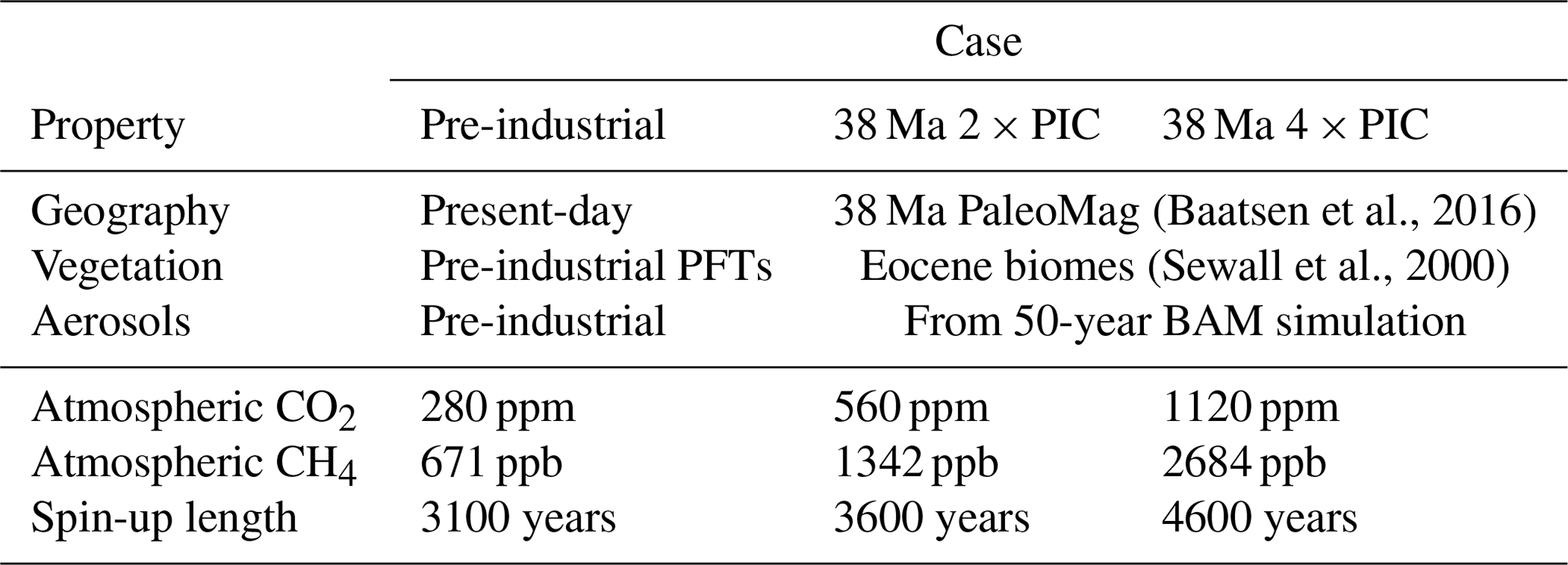
Two 38 Ma simulations are carried out with 2 × PIC and 4 × PIC, respectively, to cover the most likely range of atmospheric greenhouse gases during the middle to late Eocene (∼500–1200 ppm; Beerling and Royer, 2011; Anagnostou et al., 2016; http://www.p-CO2.org, last access: 29 November 2020) and to estimate climate sensitivity. CO₂ and CH₄ concentrations are increased simultaneously, in line with middle to late Eocene estimates (Beerling et al., 2009, 2011; Goldner et al., 2014). According to Etminan et al. (2016) the radiative forcing of 2 × PIC and 4 × PIC is equivalent to that of 2.15 × CO₂ and 4.69 × CO₂, respectively. An overview of the different model cases analysed in this paper is given in Table 1.

Table 1Overview of characteristics for all CESM 1.0.5 simulations that were performed (PFT: plant functional type, BAM: bulk aerosol model).

Download Print Version | Download XLSX

2.3 Spin-up procedure

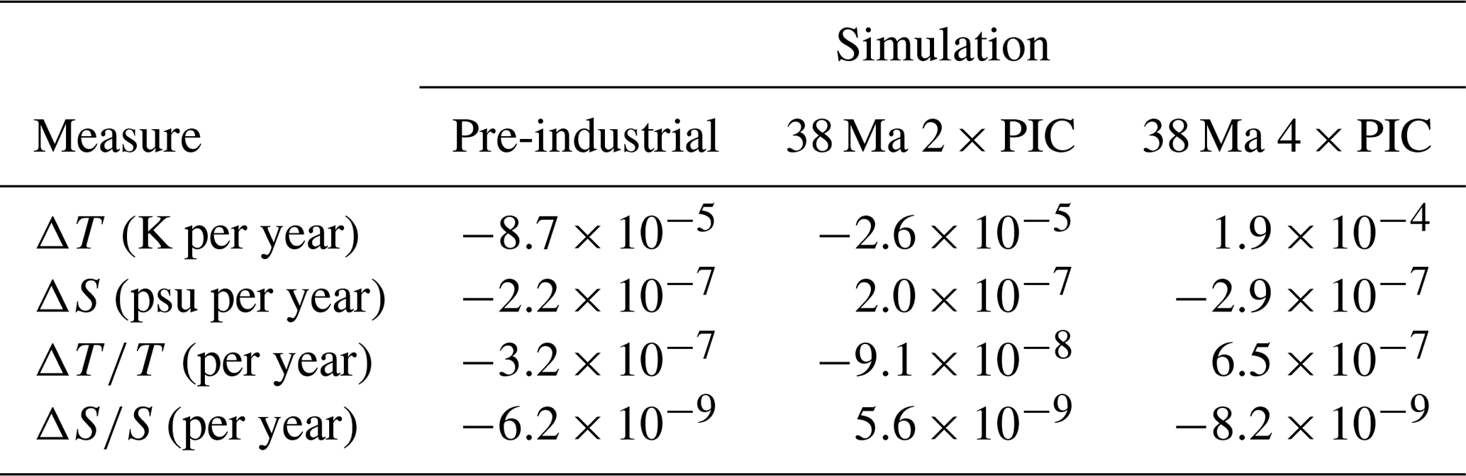
Our 38 Ma Eocene simulations are both initialised using a stagnant ocean with a horizontally homogeneous temperature distribution, decreasing with depth from 15 ^∘C at the surface to 9 ^∘C at the bottom. The pre-industrial reference is initialised using present-day temperature and salinity fields from the PHC2 dataset (Steele et al., 2001). A long spin-up (see Table 1) is performed to allow the deep ocean to equilibrate sufficiently. An overview of absolute (ΔT, ΔS) and normalised (ΔT∕T, ΔS∕S) drifts over the last 200 model years is given in Table 2 for each spin-up. Drifts are generally $\sim {\mathrm{10}}^{-\mathrm{5}}$–10⁻⁴ K per year for the global average volume-weighted ocean temperature (values of <10⁻⁴ are often regarded as well equilibrated; see e.g. Goldner et al., 2014; Hutchinson et al., 2018). Globally averaged salinity drifts at the end of all three spin-ups are $\sim {\mathrm{10}}^{-\mathrm{7}}$ psu per year.

Table 2Overview of drifts in globally averaged (full-depth, volume-weighted) ocean temperature and salinity over the last 200 model years for all three CESM spin-up simulations. Normalised drifts ΔT∕T and ΔS∕S, with T temperature in Kelvin and S salinity in practical salinity units (psu), are also shown for each case using the same interval.

Download Print Version | Download XLSX

Time series of globally averaged upper ocean (<1 km), deep-ocean (>2 km), and full-depth ocean temperatures are shown for all three spin-up runs in Fig. 2a. Starting from present-day initial conditions, the pre-industrial simulation cools down by about 0.5 ^∘C globally. The 38 Ma 2 × PIC simulation is seen to equilibrate much faster than the 4 × PIC one, probably because the deep-ocean equilibrium temperature is close to that of the initial state (∼9 ^∘C). With higher greenhouse gas concentrations, the ocean experiences additional heating at the surface, causing it to become more stably stratified which consequently reduces vertical mixing into the deep ocean. This reduced mixing in the 4 × PIC case causes the global average deep-ocean temperature to still increase about 0.1 ^∘C over the last 500 years. As expected, changes in the upper 1 km temperatures settle more quickly and are small (<0.1 ^∘C) during the last 2000 model years of each simulation.

Figure 2(a) Time series of global upper 1 km (red), below 2 km (black), and full-depth (purple) volume-weighted average temperature for the complete pre-industrial reference (dotted), 38 Ma 2 × PIC (dashed), and 4 × PIC (solid) spin-up simulations. (b) Global average near-surface air temperature for the 38 Ma cases (markers: annual, grey crosses: 2 × PIC, black dots: 4 × PIC, lines: smoothed–dashed dark blue: 2 × PIC, solid light blue: 4 × PIC), with mean values over the last 200 years given. (c) Globally integrated top-of-model net fluxes for both 38 Ma Eocene cases using the same marker and line conventions as in (b).

Download

While generally adjusting more quickly than the ocean, near-surface air temperatures can also be seen to equilibrate faster in the 38 Ma 2 × PIC case compared to the 4 × PIC one. A small but abrupt temperature drop is seen at model years 3000 and 4000 for the 2 × PIC and 4 × PIC case, respectively. This is caused by a regional shift in vegetation cover that was necessary to adjust regions of erroneously switched PFTs in the Eocene boundary conditions (Fig. S1a shows the correct vegetation cover used at the end of the 38 Ma simulations). Since most of the land surface is covered with different types of forest and the complexity of interactions with the modelled climate system is limited, the overall effect is minor. Both 38 Ma simulations were extended by another 600 years, showing little change after a quick initial adjustment. Correcting the vegetation cover mainly affects the albedo (a 1.8 × 10⁻³ increase globally), lowering the net fluxes at the top of the model atmosphere (with a net radiative forcing of about −0.1 W m⁻² and a cooling of 0.2–0.3 ^∘C; Fig. 2c). Time series of these fluxes also indicate that the atmosphere is close to radiative equilibrium towards the end of both simulations, with a <0.1 W m⁻² imbalance between globally integrated shortwave and longwave fluxes. The slightly positive radiative balance agrees with the deep ocean continuing to warm up slowly, while both the upper ocean and atmosphere show little change after model year ∼1500 for the 38 Ma 4 × PIC simulation.

In addition, global patterns of ideal age tracers (a measure for oceanic ventilation timescales; Thiele and Sarmiento, 1990; England, 1995) are observed to equilibrate over the last 1000 years of each simulation (Supplement Fig. S2) as are the meridional overturning strength and oceanic gateway transports (Supplement Fig. S3). Average values of ideal age still have considerable trends because of further ageing in stagnant deep-ocean regions (Fig. S2a) and upwelling of older water masses into the upper ocean (Fig. S2b). Such changes will likely continue for many thousands of years, but the associated circulation pattern has equilibrated by the end of each simulation, which is used for further analysis. The difference in spin-up between the two 38 Ma cases is once again highlighted in the evolution of maximum overturning strength. Whereas the 2 × PIC simulation has a stable southern overturning cell within 500 model years, its equivalent in the 4 × PIC case only materialises after 2750 years (Fig. S3b).

2.4 Proxy compilations

The 38 Ma CESM simulations presented here are validated using both qualitative and quantitative measures based on proxy records of the middle to late Eocene. After a general assessment of the model results we look more specifically at sea surface temperatures (SSTs); those from the 38 Ma 4 × PIC simulation are assumed to best represent the 42–38 Ma proxy records and from the 2 × PIC case for the 38–34 Ma interval. An overview of the considered SST proxies is given in Table S3 for 42–38 Ma and Table S4 for 38–34 Ma using data from Pearson et al. (2001, 2007), Tripati et al. (2003), Kobashi et al. (2004), Bijl et al. (2009), Liu et al. (2009), Okafor et al. (2009), Douglas et al. (2014), Hines et al. (2017), Cramwinckel et al. (2018), and Evans et al. (2018). A point-by-point comparison with proxy records is made using their estimated 38 Ma positions in accordance with the PaleoMag geography from Baatsen et al. (2016). Proxy-derived values for annual mean temperatures are considered with their calibration uncertainty for different methods (UK₃₇, TEX${}_{\mathrm{86}}^H$, Mg ∕ Ca, Δ₄₇, and δ¹⁸O). Modelled SSTs at the reconstructed proxy locations are given with error bars representing the variance in a surrounding 4^∘ × 4^∘ box, covering the uncertainty associated with the palaeogeographic reconstruction (http://www.paleolatitude.org, last access: 29 November 2020). Estimates using UK₃₇ are disregarded at low latitudes as the calibration saturates at ∼28 ^∘C (Conte et al., 2006). There is an ongoing discussion on which calibration to use for TEX₈₆ (O'Brien et al., 2017; Cramwinckel et al., 2018; Hollis et al., 2019). In addition to SST estimates using the exponential TEX${}_{\mathrm{86}}^H$ calibration from Kim et al. (2010), we show those using the linear relation of Kim et al. (2008) (light blue markers in Fig. 6). There is also uncertainty in the calibration of Mg ∕ Ca, for which we use the constraints on seawater chemistry from Evans et al. (2018).

In addition to SSTs, we compare modelled near-surface air temperatures to terrestrial proxies. Similarly, the distinction is made between the late middle Eocene (∼42–38 Ma) and late Eocene (∼38–34 Ma) as a reference for the 38 Ma 4 × PIC and 2 × PIC simulations, respectively. The considered records are listed in Tables S5 and S6, containing data from Greenwood and Wing (1995), Gregory-Wodzicki (1997), Smith et al. (1998), Wolfe et al. (1998), Greenwood et al. (2004), Retallack et al. (2004), Hinojosa and Villagrán (2005), Uhl et al. (2007), Boyle et al. (2008), Schouten et al. (2008), Prothero (2008), Eldrett et al. (2009), Quan et al. (2012), and Passchier et al. (2013). Terrestrial proxies used here consist of vegetation-based indicators using pollen, nearest living relative (NLR), leaf physiognomy (LMA, CLAMP, ELPA, and LMA; Wing and Greenwood, 1993; Yang et al., 2011; Traiser et al., 2005; Kowalski and Dilcher, 2003), and MBT–CBT (Peterse et al., 2012).

2.5 Previous model results

The results of our 38 Ma simulations are compared to those of Goldner et al. (2014) (hereafter: GH14) and Hutchinson et al. (2018) (H18). The latter provides an opportunity to test the robustness of the overall temperature distribution in the modelled middle to late Eocene cases using very similar boundary conditions but a different model. Here, we are mainly looking at zonally averaged sea surface and near-surface air temperatures and how they correspond to the previously presented proxies. A side-by-side overview of oceanic and atmospheric fields from this study and GH14 can be found in the Supplement.

The simulations of GH14 were carried out with the CCSM3, a predecessor of the CESM1 (the former having CAM3 rather than CAM4 with a spectral versus finite-volume core, respectively). GH14 used a 45 Ma hot-spot-referenced reconstruction for their geographical boundary conditions, in which Antarctica is shifted by ∼6^∘ latitude compared to the 38 Ma PaleoMag reconstruction used here. They applied four subsequent doublings of pre-industrial CO₂ levels, which correspond to the EO1–EO4 cases of Cramwinckel et al. (2018). In terms of horizontal resolution GH14 implemented ∼2.5 and 3.7^∘ for the model's ocean and atmosphere grids, respectively, versus ∼1 and ∼2^∘ here.

A model set-up similar to ours was implemented by H18 using the 38 Ma geography reconstruction from Baatsen et al. (2016), a similar oceanic resolution (∼1^∘ – atmosphere: ∼3^∘), and a vegetation cover based on the same biome distribution used here (Fig. S1a). They studied mostly the late Eocene using the GFDL CM2.1 and subsequent doublings of present-day rather than pre-industrial CO₂ concentrations (i.e. ∼400 ppm).

A more quantitative assessment of the model's performances is made following a procedure similar to the one presented by Lunt et al. (2012) using the SST proxy compilations considered here (Tables S3 and S4). The model–proxy discrepancy σ is defined as the average difference between model-predicted and proxy-induced SSTs at reconstructed locations (using 38 Ma PaleoMag for this study and H18 versus 45 Ma hot spot for GH14). A set of different comparisons is considered using either all proxies or a subset (i.e. global, equatorial, or extra-tropical) and modelled annual mean versus summertime temperatures. An absolute error $\left|\mathit{\sigma }\right|$ is also introduced (rather than e.g. RMS) to rule out better scores by compensating for errors without exaggerating the impact of a single (possibly unrealistic or not representative) proxy value.

2.6 Climate sensitivity

A number of additional simulations are carried out to determine the model's response to an altered radiative forcing when only the concentration of atmospheric greenhouse gases is changed. These include a 2000-year 4 × CO₂ (Fig. S16) and four 20-year perturbation experiments listed below. Using the extrapolation method introduced by Gregory et al. (2004) on the results of those shorter simulations (see Fig. S17 for 4 × CO₂), the model-derived radiative forcing from consecutive doublings of either CO₂ or both CO₂ and CH₄ is determined as (bracketed values: theoretical estimates from Etminan et al., 2016; E16)

• 1 × CO₂→ 2 × CO₂: ΔRF${}^{\mathrm{2}\times {\mathrm{CO}}_{\mathrm{2}}}=$ 3.49 W m⁻²
  (E16: 3.80 W m⁻²),

• 1 × CO₂→ 4 × CO₂: ΔRF${}^{\mathrm{4}\times {\mathrm{CO}}_{\mathrm{2}}}=$ 7.93 W m⁻²
  (E16: 7.96 W m⁻²),

• 1 × PIC → 2 × PIC: ΔRF${}^{\mathrm{2}\times }=$ 4.18 W m⁻²
  (E16: 4.23 W m⁻²),

• 1 × PIC → 4 × PIC: ΔRF${}^{\mathrm{4}\times }=$ 9.33 W m⁻²
  (E16: 8.96 W m⁻²).

The value of ΔRF${}^{\mathrm{2}\times {\mathrm{CO}}_{\mathrm{2}}}$ determined here is slightly lower than the 3.8 W m⁻² estimated by E16 but very close to the 3.5 W m⁻² reported by Kay et al. (2012) using offline radiative transfer calculations for CAM4 specifically. Note that the model-derived radiative forcing is generally close to the corresponding one from E16 but featuring a stronger nonlinear behaviour towards higher perturbations, especially when including the effect of CH₄. Using the values shown above, the radiative forcing that results only from a second PIC doubling can thus be estimated as ΔRF${}_{\mathrm{2}\times }^{\mathrm{4}\times }=$ 5.15 W m⁻² (=ΔRF${}^{\mathrm{4}\times }-\mathrm{\Delta }$RF^2×). Through a (log-scaled) quadratic fit, these estimates can also be used to show that our 2 × PIC is equivalent to 2.25 × CO₂, while 4 × PIC corresponds to 4.85 × CO₂ (rather than 2.15 and 4.69 based on E16, respectively).

Starting from the equilibrated pre-industrial reference (at model year ∼3100), an instant quadrupling of atmospheric CO₂ was applied and continued for another 2000 model years. Using the same procedure as Gregory et al. (2004), the equilibrium climate sensitivity (ECS) of the model was assessed at 3.17 ^∘C per CO₂ doubling. The first 100 model years are disregarded in the extrapolation to better capture the effect of slow feedbacks (see Fig. S16). Using the same atmospheric configuration and a slab ocean model, Bitz et al. (2012) reported a comparable ECS of 3.1 ^∘C in the CCSM4. With the model-derived radiative forcing of 7.93 W m⁻² and an extrapolated equilibrium response of 6.34 ^∘C, the normalised equilibrium climate sensitivity of the pre-industrial reference is therefore S_PI= 0.80 ^∘C W⁻¹ m².

Since we carry out a long spin-up simulation for each of the 38 Ma cases, we can determine the equilibrium climate response as the difference between the actual equilibrium states rather than making an estimate through extrapolation. The mean over the last 200 (rather than 50 for the other results) model years of each simulation is taken to exclude as much of the internal variability as possible. When comparing global average temperature differences between the pre-industrial reference and both Eocene simulations, not all of the warming is a result of higher greenhouse gas concentrations. To separate the internal effect of palaeogeography from the externally (i.e. greenhouse gas) driven warming, the 38 Ma Eocene equilibrium climate sensitivity S_EO can also be calculated using the combined radiative forcing due to greenhouse gas and palaeogeography changes by assuming that

where ΔT is the temperature difference between two climatic states, ΔRF the net radiative forcing from greenhouse gases, and G the radiative forcing due to the (integral) effect of palaeogeography. Note that the latter also includes changes in the distribution of e.g. land ice and vegetation, as those are applied boundary conditions in the model set-up used here. In order to be compatible with S_PI, this formulation returns S in normalised units of [^∘C W⁻¹ m²] rather than [^∘C per CO₂ doubling] as used by Royer et al. (2012).

Since both 38 Ma Eocene simulations use the same boundary conditions (except CO₂ and CH₄ concentrations), it is reasonable to assume that S and G estimated from the comparison with the pre-industrial case should be similar (provided that their nonlinear contribution is small). By comparing the temperatures of both Eocene runs to those of the pre-industrial reference, G can then be estimated from

where ΔT^4× and ΔT^2× denote the temperature difference with respect to the pre-industrial climate for the 38 Ma 4 × PIC and 2 × PIC case, respectively. Within this formulation, globally averaged near-surface air temperatures can then be substituted by equatorial (<23.5^∘ N or S) SSTs (with a 3∕2 ratio between global and equatorial change suggested by Royer et al., 2012) or deep-sea temperatures, which should both be more compatible with ECS estimates from proxy data.

3.1 The simulated middle to late Eocene equilibrium climate

Taking the mean over the last 50 years of the 38 Ma 4 × PIC simulation, a number of annual mean oceanic fields are shown in Fig. 3 (see also Fig. S4 for the pre-industrial reference and Fig. S5 for the 38 Ma 2 × PIC case; seasonal fields are shown in Fig. S8). Sea surface temperatures are quite warm at low latitudes (34 ^∘C on average, regionally >36 ^∘C) but also mild across high latitudes (Fig. 3a). The Southern Ocean, especially its Pacific part, is mainly characterised by annual mean temperatures of 10–20 ^∘C, while those of the Arctic Ocean are mostly 6–10 ^∘C. The former Neo-Tethys (Pacific-Indian-Mediterranean) Ocean still mostly acts as one basin in the equatorial region, with an expansive warm pool and cold tongue across its western and eastern part, respectively.

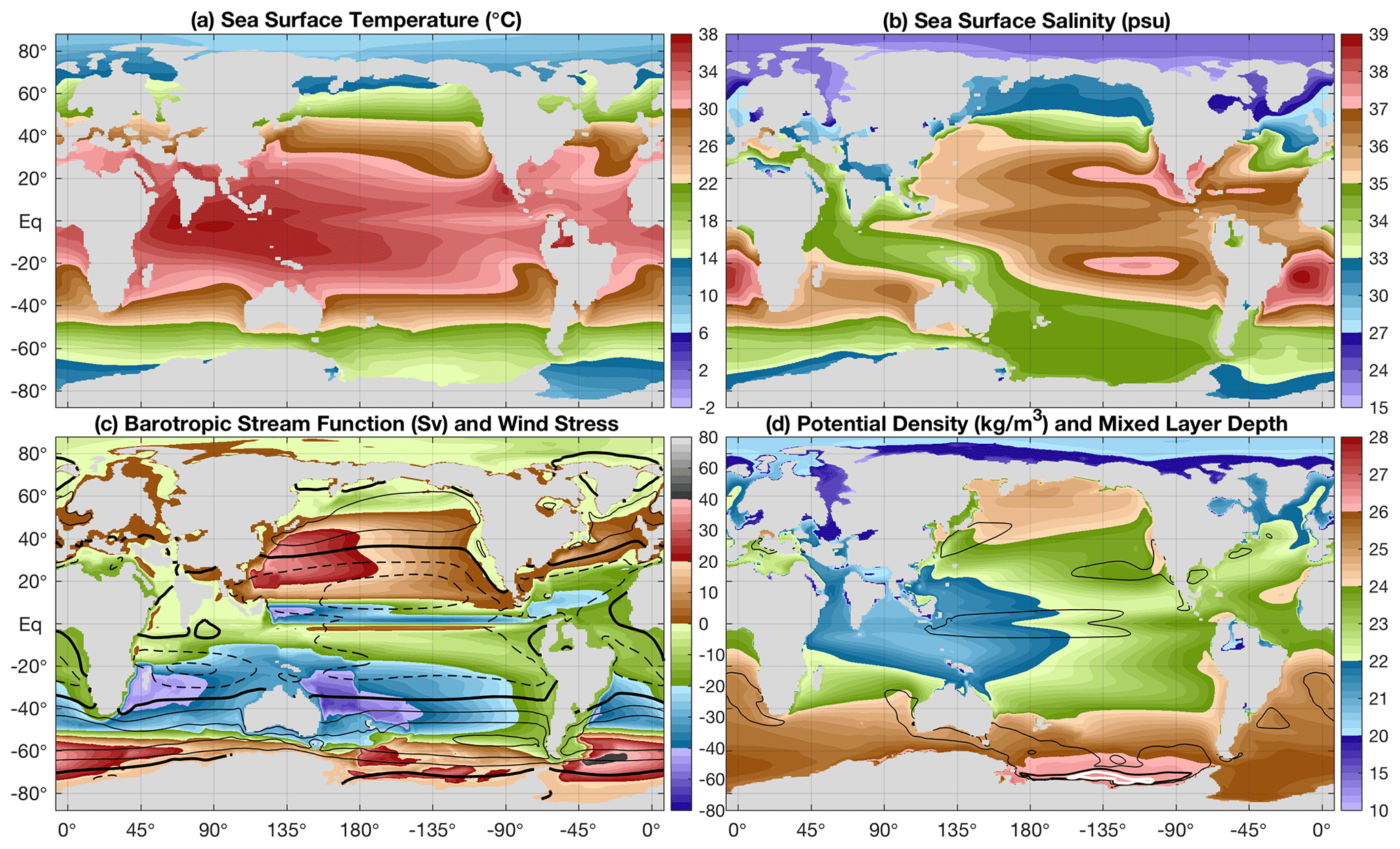
Figure 3Annual mean for the 38 Ma 4 × PIC simulation with (a) sea surface temperature and (b) salinity, (c) barotropic stream function (positive for clockwise flow) and zonal wind stress (contours every 4 × 10⁻² Pa, solid positive and dashed negative, thick line at 0 Pa), and (d) upper 200 m average potential density and mixed layer depth (contours at 100 and 250 m, thick white line at 500 m).

Mild temperatures in the sub-polar South Pacific are accompanied by relatively high salinities of around 35 psu (Fig. 3b). Higher salinities are present across low-latitude evaporative regions around the world, in contrast to the much fresher Arctic Ocean (∼20 psu). The latter is geographically almost isolated and only connected to the shallow Para-Tethys by the Turgai Strait (<100 m depth) and through the Nordic Seas (<1 km depth) to the North Atlantic Ocean where consequently low surface salinities are seen as well.

The surface temperature and salinity patterns are reflected by upper 200 m potential density (Fig. 3d), with high values throughout the Southern Ocean and much lower densities and thus more stably stratified waters across the North Atlantic and Arctic Ocean. Deepwater formation occurs only in the Pacific sector of the Southern Ocean in winter (at ∼11.4 ^∘C and 34.8 psu), but high upper-level densities suggest that this may take place virtually anywhere around the Antarctic continental slope. The only part of the Northern Hemisphere where deepwater formation could occur is the high-latitude Pacific Ocean, but it is never seen in either of the 38 Ma simulations.

The global ocean circulation consists mostly of expansive sub-tropical gyres, a geographically restricted Antarctic Circumpolar Current (ACC), and some rather weak sub-polar gyres (Fig. 3c). This proto-ACC is associated with a sharp frontal zone separating warm sub-tropical from cooler sub-polar waters. Even with a shallow Drake Passage and Tasmanian Gateway (200–500 m; see Fig. 1a, d), the integrated zonal flow is about 25 %–30 % of its pre-industrial equivalent (45–50 Sv vs. 180 Sv; see also Fig. S3a). Strikingly, the temperature front is located at 55–60^∘ S, which is almost 10^∘ poleward of where it is found in the pre-industrial reference (Fig. S4). The zonal variability in the location of the front also has profound implications for regional meridional temperature contrasts. This location is strongly bound by the zonal wind stress maximum, indicating that it is fixed by the latitudes where both atmospheric and oceanic flow are the least obstructed by continents.

Despite differences in spin-up time, patterns of the equilibrium ocean circulation state are generally similar for our 38 Ma 2 × PIC and 4 × PIC simulations (see also Fig. S5). The annual mean global average sea surface temperature (SST) is 28.4 ^∘C in the 4 × PIC case versus 25.7 ^∘C in the 2 × PIC one and 18.4 ^∘C in the pre-industrial reference (Table ). Similar temperature differences of 2.5–3 ^∘C are seen in both the upper and deep ocean between the 38 Ma cases (Fig. 2a). Globally averaged deep-sea temperatures (below 2 km) reach ∼11.5 ^∘C in the 38 Ma 4 × PIC case and ∼8.6 ^∘C in the 2 × PIC one, which is much warmer than for the pre-industrial ocean (∼0.7 ^∘C). The difference in equatorial (<23.5^∘ N or S) SSTs between the Eocene cases and the pre-industrial reference is smaller (i.e. 2–3 ^∘C less than the other measures listed) but still considerable.

Table 3Mean equilibrium temperatures over the last 200 model years of each simulation, showing MAT_glob: global average air temperature (at 2 m reference height), SST_glob: global average sea surface temperature, SST_eq: equatorial (<23.5^∘ N or S) average SST, and T_deep: global average deep-ocean temperature (below 2 km).

Download Print Version | Download XLSX

Also for the atmospheric fields, the mean over the last 50 years of the 38 Ma 4 × PIC simulation is taken and shown in Fig. 4 (see also Fig. S6 for the pre-industrial reference and Fig. S7 for the 38 Ma 2 × PIC case; seasonal fields of 4 × PIC are shown in Fig. S9). As for the ocean, the modelled 38 Ma 2 × PIC atmosphere (Fig. S7) is quite similar to the 4 × PIC one. At 23.34 ^∘C the globally averaged annual mean near-surface air temperature at 2 × PIC is ∼3.2 ^∘C cooler than at 4 × PIC (26.55 ^∘C). This is, however, still ∼9.5 ^∘C warmer than in the pre-industrial reference (13.82 ^∘C).

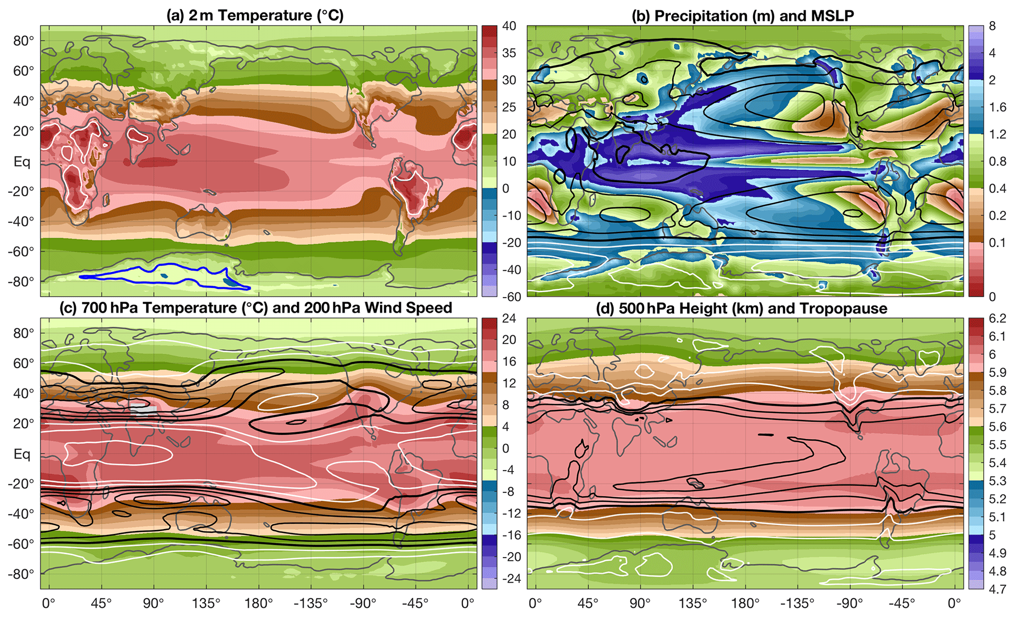
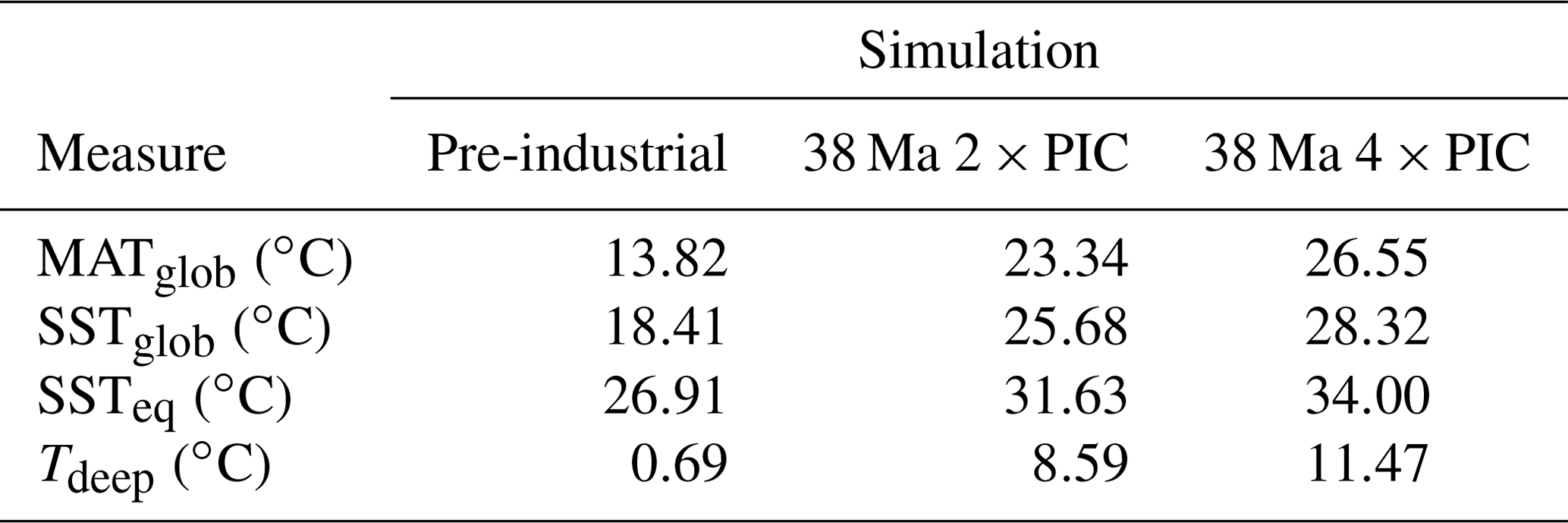
Figure 4Annual mean for the 38 Ma 4 × PIC simulation with (a) near-surface (2 m) air temperature (shading) and min–max temperature (contours; blue for T_min<0 ^∘C and white for T_max>40 ^∘C), (b) precipitation (shading) and mean sea level pressure (MSLP; contours every 5 hPa, thick black lines every 20 hPa, ≥1000 hPa in black and <1000 hPa in white), (c) 700 hPa temperature (shading) and 200 hPa wind speed (contours every 5 m s⁻¹ starting at 10 m s⁻¹; white for <20 m s⁻¹ and black for ≥20 m s⁻¹, thick black lines every 20 m s⁻¹), and (d) 500 hPa geopotential height (shading) and tropopause height (contours every 1 km; white for <15 km and black for ≥15 km, thick black line at 15 km).

The simulated Eocene climate is overall warmer and wetter than that of the pre-industrial reference, with reduced contrasts between low and high latitudes. Near-surface air temperatures (at 2 m; Fig. 4a) under 4 × PIC are above zero and up to 40 ^∘C over land at low latitudes in the annual mean (with summer maxima regionally >50 ^∘C; see Fig. S9a, b). Annual mean (daily) minimum temperatures are only below freezing in East Antarctica and northeast Siberia (the latter only at 2 × PIC). Extreme seasonality is seen over the continental interior of Antarctica (Fig. S9a, b), with 35–45 ^∘C differences between daily mean summer and winter temperatures.

Simulated precipitation and mean sea level pressure (MSLP) patterns (Fig. 4b) indicate the presence of a prominent tropical trough and expansive sub-tropical ridges in the Eocene. The inter-tropical convergence zone (ITCZ) consists of two precipitation maxima extending over the Indo-Pacific basin on both sides of the Equator. A pronounced double ITCZ over the Pacific Ocean is also seen in the pre-industrial reference (Fig. S6b) and a known model-related issue (Song and Zhang, 2009; Bellucci et al., 2010). Effects of orographic lift are evident on westward-facing coastlines and mountain ranges across middle and high latitudes (e.g. southern Andes and northern Rocky Mountains). Regardless of an overall reduced Equator-to-pole temperature gradient in the 38 Ma 4 × PIC case, middle-latitude storm tracks are prominent with increased precipitation and a poleward expansion with respect to the pre-industrial reference. Strong seasonality in the precipitation patterns also indicates the importance of monsoons in this warm Eocene climate (Fig. S9c, d).

The modelled 700 hPa temperature (Fig. 4c) of the 38 Ma 4 × PIC case highlights warm mid-level air masses in persistent continental high-pressure regions in the sub-tropics. The air over Antarctica is substantially warmer than over the Arctic because of its elevation and continental climate. Like the Tibetan Plateau today, the Antarctic continent therefore acts as an elevated heat island in summer (Hoskins and Karoly, 1981; Ye and Wu, 1998; Fig. S9f). Wind speeds at 200 hPa highlight the positions of both sub-tropical and polar jet streams. Several wind maxima, related to (mostly topographically induced) preferred Rossby wave activity, are evident but most pronounced at ∼90^∘ E. A comparable jet stream pattern with regional wind maxima is seen in the pre-industrial reference, but it is more zonally uniform and shifted equatorward.

Reduced latitudinal and hemispheric differences in the modelled 38 Ma 4 × PIC compared to the pre-industrial reference are also seen in 500 hPa geopotential and tropopause heights (Fig. 4d). The latter is defined using the WMO definition of a −2 ^∘C km⁻¹ lapse rate. Both fields show a nearly meridionally symmetric pattern for the Eocene, with the sharpest gradient across middle-latitude regions. The overall warmer air column in the Eocene case accounts for an increase in the 500 hPa surface by 100–200 m (up to 400 m over Antarctica) and the tropopause by 1–2 km.

We assess the global heat budget in our model results by looking at both the oceanic and atmospheric heat transports, along with their link to global circulation patterns, presented in Fig. 5. The globally integrated oceanic meridional overturning stream function is similar in pattern and extent (Fig. 5a) for both 38 Ma Eocene simulations but different to that of the pre-industrial reference (Fig. 5b). Little change in shallow wind-driven cells around the Equator is seen among all three cases. A deep meridional overturning cell is present in the Southern Hemisphere rather than the Northern Hemisphere in the 38 Ma configuration, which is slightly stronger and deeper in the 2 × PIC case. The effect of upwelling due to (Ekman pumping by) the zonal flow in the (proto-)ACC can be seen at around 55^∘ S in both 38 Ma cases as well as in the pre-industrial reference. The related overturning cell in the latter is much deeper and stronger as a result of a more developed ACC but mostly the unrestricted zonal flow in the present geographical configuration. Note that the average latitudinal shift of these overturning cells between the modelled Eocene and pre-industrial circulation is less pronounced than the more regional variations of the surface polar front in Figs. 3 and S4.

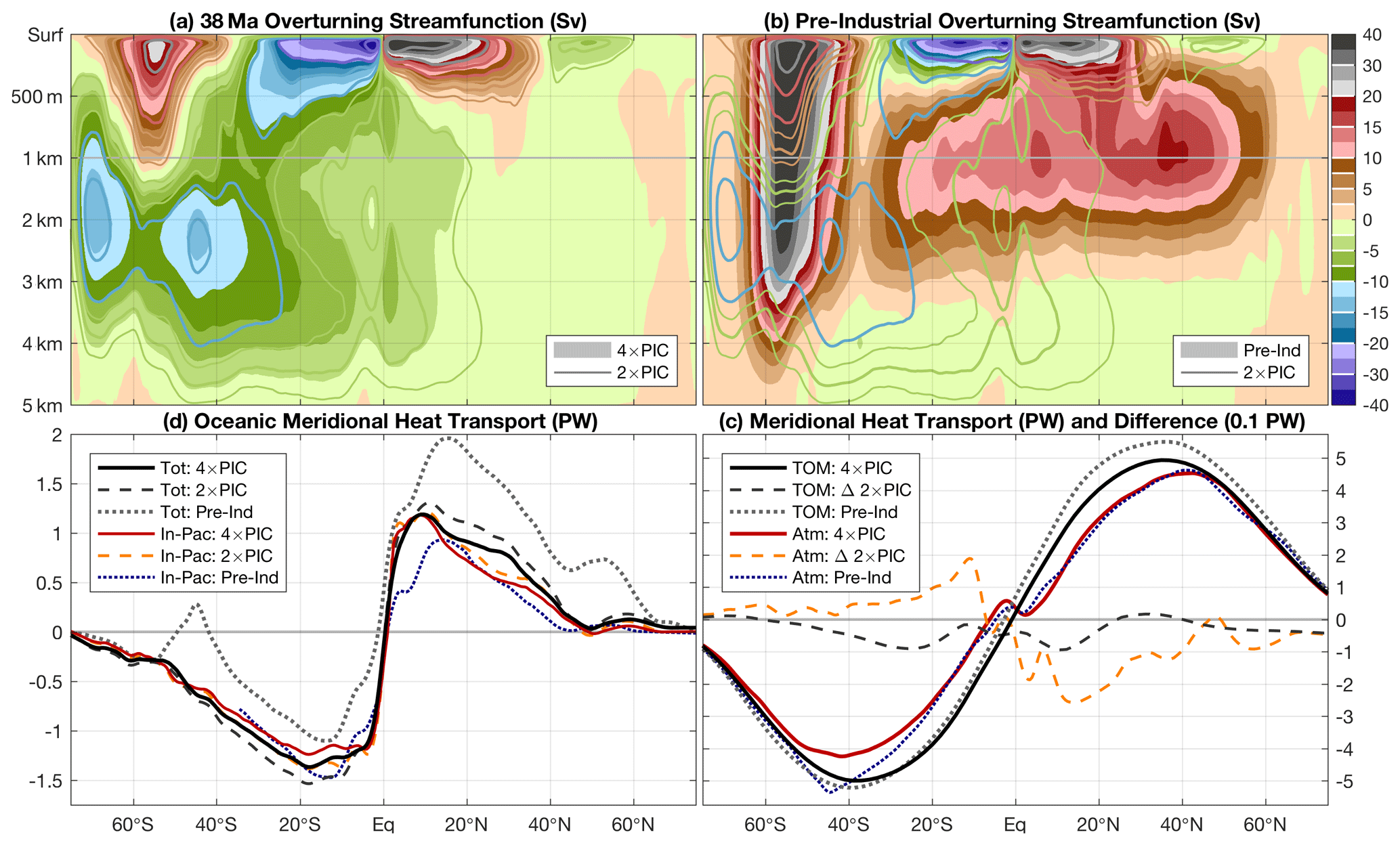
Figure 5Global oceanic meridional overturning stream function averaged over the last 50 model years of the (a) 38 Ma 4 × PIC (shading) and 2 × PIC (contours) simulations as well as the (b) pre-industrial reference (shading; 38 Ma 2 × PIC again in contours). Contours are drawn using the same colour scale at levels indicated by white lines in the colour bar to the right. (c) Integrated meridional heat transport in the ocean, globally (greyscale) and Indo-Pacific only (coloured) for the three model cases. Note that the horizontal (latitude) scale covers the range [75^∘ S, 75^∘ N], with latitude increasing from left to right, for a better comparison with oceanic fields in (a) and (b). The top-of-model (TOM) required total meridional heat transport is shown in (c) for 38 Ma 4 × PIC (solid black) and the pre-industrial reference (dotted grey) with the corresponding atmospheric component in red (4 × PIC) and dotted blue (pre-industrial). Differences with respect to 38 Ma 4 × PIC for both total (dashed dark grey) and atmospheric (dashed orange) heat transport are given for the 2 × PIC case, magnified 10-fold.

Download

An otherwise predominantly wind-driven gyre circulation in the 38 Ma simulations is reflected by symmetric oceanic meridional heat transport into both hemispheres (Fig. 5c). This is in contrast to the pre-industrial situation, in which a difference of up to 1 PW is seen between hemispheres, making the Northern Hemisphere relatively warm (Trenberth and Caron, 2001). A major part of the 38 Ma oceanic heat transport occurs in the Neo-Tethys–Indo-Pacific Ocean, indicating the dominant role of this basin within the Eocene circulation. The presence of a deep overturning cell in the North Atlantic Ocean in the pre-industrial reference substantially reduces the relative Indo-Pacific contribution. The largest relative differences between hemispheres are seen at high latitudes, where about 0.5 PW is transported southward at 45^∘ S, while the heat transport is close to zero at 45^∘ N in both 38 Ma cases. This difference can be explained by the presence of a deep southern overturning cell, pulling warm waters into the southern high latitudes.

To determine the total required meridional heat transport, the top-of-model net radiative flux is integrated zonally (Fig. 5d). Overall differences are small between the 38 Ma cases and pre-industrial reference, with a slight shift towards the Southern Hemisphere, making the Eocene pattern more symmetric. Changes seen in oceanic meridional heat transport are less pronounced in the total transport and are thus compensated for by the atmospheric component, albeit only partially. This suggests that the reduced latitudinal temperature gradient seen in the modelled 38 Ma cases is thus not sustained by increased meridional heat transport, but rather induces a reduced transport with respect to the pre-industrial reference.

3.2 Model–proxy comparisons

In terms of the general ocean circulation, proxy-based information is limited but mostly agrees well with what is shown by the model. Persistent deepwater formation in the South Pacific Ocean throughout most of the Eocene and the possibility of a North Pacific or South Atlantic source are consistent with the findings of Cramer et al. (2009) and Hague et al. (2012). A strongly stratified North Atlantic Ocean with low-salinity waters at middle to high latitudes was also suggested by Coxall et al. (2018) prior to ∼36 Ma.

The all but complete absence of Arctic sea ice in the 38 Ma 4 × PIC model results differs from indications of seasonal sea ice during the middle Eocene by Stickley et al. (2009). Although limited in extent, the model does show sea ice during the winter months under 2 × PIC (contours in Fig. S5). In addition to the sea ice indications being highly localised, age restrictions on the considered section of the ACEX core make it difficult to rule out whether the sea ice actually occurred in the late Eocene. Still, the model's limitations to represent sea ice need to be considered here, as the applied scheme is quite simple. Low salinities across the Arctic Ocean would have made it easier for sea ice to form, which is not reflected by the implemented fixed SST threshold (−1.8 ^∘C).

A southward migration of the temperature front in the Southern Ocean can help to explain some of the high SSTs induced from proxies, especially across the southwest Pacific region (Bijl et al., 2009; Hines et al., 2017). Additionally, zonal variations in the front induce a thermal heterogeneity in the Southern Ocean. The 6–8 ^∘C (Fig. 3a) difference between Tasmania and the tip of the Antarctic Peninsula (Seymour Island) agrees well with proxy indications from Douglas et al. (2014). A 10–15^∘ latitude difference between Tasmania and the tip of the Antarctic Peninsula in the (PaleoMag) geography reconstruction used (Baatsen et al., 2016) here may help to explain the temperature differences seen in proxies. On the other hand, eastward flow through the Tasmanian Gateway limits the strength and extent of the Antarctic countercurrent around most of Antarctica (Bijl et al., 2013; Houben et al., 2019). The model results disagree with indications of a strong sub-polar gyre in the Ross Sea (limited in the model by the northern extent of East Antarctica) into the late Eocene, with predominantly westward flow through the Tasmanian Gateway and Antarctic-derived surface waters found in the southwest Pacific Ocean (Stickley et al., 2004; Huber et al., 2004; Bijl et al., 2013; Cramwinckel et al., 2020). The absence of a clear temperature discrepancy between the two sides of the gateway still suggests a strong connection as seen in the model (Bijl et al., 2013), possibly explained by atmospheric influences at shallow and near-coastal locations.

In Fig. 6a point-by-point comparison with available SST proxies (see also Table S3) is complemented by zonally averaged SSTs from the model along with their longitudinal spread for both the annual and summer mean (for 38 Ma 4 × PIC; see also Fig. S10 for 2 × PIC).

Figure 6Zonal average annual mean (black) and summer mean (red) sea surface temperature (SST), with shaded regions showing minimum and maximum values for each latitude, from the 38 Ma 4 × PIC simulation. Blue markers indicate estimates from 42–38 Ma SST proxies (see also Table S3; light blue: linear, dark: log calibration from Kim et al., 2008, for TEX${}_{\mathrm{86}}^H$), whereas the white (annual) and red (summer) circles depict model values at the corresponding 38 Ma locations. Error bars are obtained using proxy calibration errors and the spatial variation within a 4^∘ × 4^∘ box surrounding the corresponding location in the model. The inset shows a scatter plot comparing proxy and model SST, with dashed lines indicating a linear fit using annual mean (black) or summer mean (red; only poleward of 23^∘ N or S) model temperatures.

Download

For low-latitude regions, model results and proxies are generally in good agreement (i.e. within uncertainty). Some near-equatorial sites (e.g. Atlantic ODP Sites 925, 929, and 959) show cooler temperatures than suggested by the model of around 30 ^∘C (when considering TEX${}_{\mathrm{86}}^H$). Both the model's limitations representing the sharp upwelling region and uncertainty in the palaeolatitude can explain this offset. Cooler near-equatorial temperatures (down to <30 ^∘C) are in fact indicated by the increased zonal spread, showing that these are possible in the simulated Eocene climate. TEX${}_{\mathrm{86}}^H$ estimates from Tanzania and recent clumped isotope measurements from Java suggest that SSTs of ∼35 ^∘C or more are possible outside upwelling regions, which is well in line with the 38 Ma 4 × PIC results.

Mixed agreement is seen at other latitudes, with model results seemingly too warm at northern middle latitudes, too cold at southern middle latitudes, and good at high latitudes. The large discrepancy with proxy estimates from the Gulf of Mexico and Neo-Tethys (Mediterranean) stands out. While it seems unlikely that these regions would be colder in the Eocene than they are today, the model probably underestimates strong seasonal cooling in shallow coastal waters and other localised effects near the coastline due to the complex palaeogeography at both locations. SST estimates from other locations at a similar latitude, such as ODP Site 1052 on Blake Nose (east of Florida), are much higher, bringing them back into good agreement with the model.

An improved match is generally found at most southern middle and high southern latitudes when modelled summertime temperatures are considered. Since SST proxies are based on past living organisms, they possibly have a bias towards the warm season as their activity and sedimentation are directly or indirectly affected by the available amount of sunlight (Sluijs et al., 2006, 2008; Bijl et al., 2009; Hollis et al., 2012; Schouten et al., 2013). Confidence in the modelled annual mean SSTs is boosted by nearly perfect agreement in the Arctic and clumped isotope indicators elsewhere (UK and Seymour Island).

The modelled 38 Ma 2 × PIC SSTs similarly show overall good agreement with 38–34 Ma proxy estimates, with a higher spread in the latter (Fig. S10 and Table S4). The best overlap is again seen in low-latitude regions, as is a better match with modelled summer temperatures at high latitudes (except for clumped isotopes). Considering the model's limitations and uncertainties or possible biases in proxy-derived SST estimates, these 38 Ma simulations can reconstruct the middle to late Eocene (42–34 Ma) temperature distribution well.

Despite the limited latitudinal coverage of terrestrial proxies, overall good agreement is also seen between the modelled temperatures on land (Fig. S11 for 38 Ma 4 × PIC; see also Fig. S12 for 2 × PIC). Proxy estimates from China, however, indicate little change in temperature, while the model shows considerably warmer conditions at lower latitudes. Quan et al. (2012) discuss the limitations of capturing high summer temperatures, as it is unlikely to see similar conditions over a >20^∘ latitude range. There are currently no proxy indications to assess the possibility of very high model-based temperatures (exceeding 50 ^∘C; see Fig. S9a, b) in low-latitude continental interiors. An important limitation of the model, especially on land, is its resolution, which smoothens the topography and therefore underestimates local temperature effects. A correction using the original 0.1^∘ geography reconstruction from Baatsen et al. (2016) and a free tropospheric lapse rate of −6.5 K km⁻¹ significantly improves the agreement between modelled and proxy-based temperatures, especially in North America (small squares versus filled markers in the inset of Fig. S11).

3.3 Model–model comparisons

Zonally averaged SSTs of our 38 Ma 4 × PIC and 2 × PIC simulations are compared to those of the 4 × CO₂ (i.e. 1120 ppm) case from GH14 and the 800 ppm CO₂ (i.e. 2× PD) case from H18 in Fig. 7, along with the pre-industrial reference and the available middle to late Eocene proxies. A similar overview considering near-surface air temperatures and terrestrial proxies can be found in Fig. 8. All of the Eocene cases feature an overall warming compared to the pre-industrial reference, which is the strongest over southern high latitudes, along with a reduction of the Equator-to-pole temperature gradient. Both of our 38 Ma cases and the 800 ppm simulation of H18 are considerably warmer than the 45 Ma 4 × CO₂ of GH14, indicating a higher sensitivity to the applied Eocene boundary conditions. It is important to mention that the simulations of H18 show deepwater formation in the North Pacific Ocean, in addition to the Southern Ocean as found here and in GH14. This results in a zonal variation of northern high-latitude SSTs, but little change is seen (outside the Arctic Ocean) in zonally averaged profiles in Fig. 7.

Figure 7Annual mean zonal average sea surface temperature for the 38 Ma 4 × PIC (black; this study), 2 × PIC (green; this study), 45 Ma 4 × CO₂ (dashed red; GH14 – Goldner et al., 2014), 38 Ma 2 × CO₂ (i.e. 800 ppm, dash-dotted magenta; H18 – Hutchinson et al., 2018), and pre-industrial reference (dotted blue; this study) simulations. Estimates from proxy data are represented by blue squares for 42–38 Ma and circles for the 38–34 Ma period. Shading indicates the zonal range in temperatures for both the 38 Ma 4 × PIC (grey) and 45 Ma 4 × CO₂ (yellow) case; thin lines show the highest summer temperatures at each latitude (light grey shading added for 38 Ma 4 × PIC).

Download

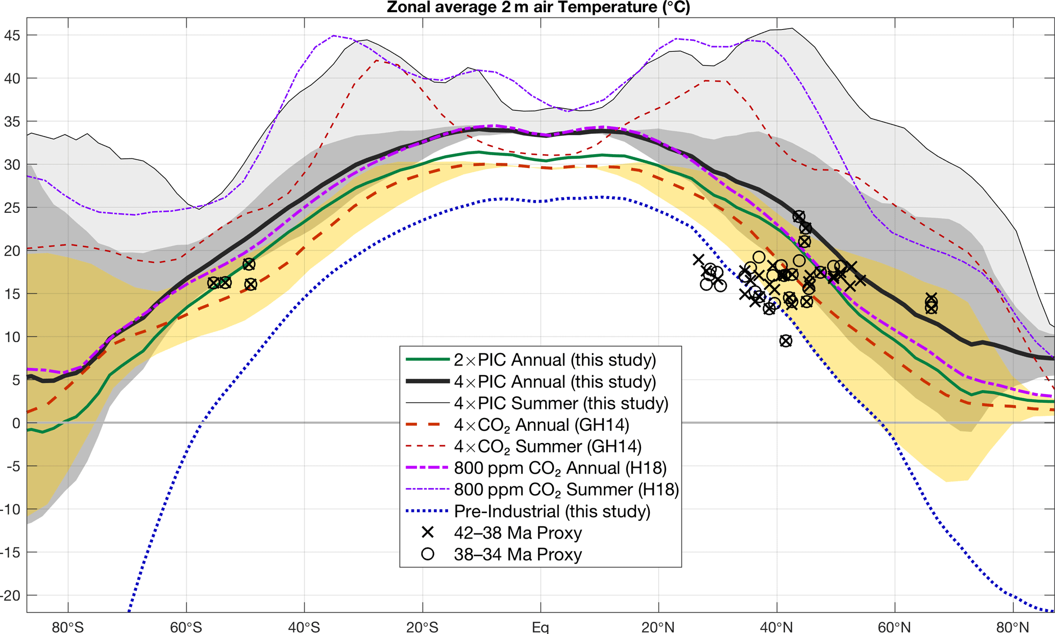
Figure 8Annual mean zonal average near-surface (2 m) air temperature for the 38 Ma 4 × PIC (black; this study), 2 × PIC (green; this study), 45 Ma 4 × CO₂ (dashed red; GH14 – Goldner et al., 2014), 38 Ma 2 × CO₂ (i.e. 800 ppm, dash-dotted magenta; H18 – Hutchinson et al., 2018), and pre-industrial reference (dotted blue; this study) simulations. Estimates from proxy data are represented by crosses for 42–38 Ma and circles for the 38–34 Ma period. Shading indicates the seasonal (DJF, JJA) range in temperatures for both the 38 Ma 4 × PIC (grey) and 45 Ma 4 × CO₂ (yellow) case; thin lines show the highest summer temperatures at each latitude (light grey shading added for 38 Ma 4 × PIC).

Download

The most prominent differences in geography between the 45 Ma GH14 and our 38 Ma simulations are in the representation of Antarctica, the Tasmanian Gateway opening, and the position of India. The Southern Ocean in particular shows large differences in circulation and the resulting temperatures, mainly related to the different model geographies. The formation of a proto-ACC and southern extent of the East Australia current act to shift the polar front in the South Pacific southward for the 38 Ma cases, while the opposite happens for 45 Ma (Fig. S13). The southward expansion of sub-tropical gyres and migration of the associated temperature front seen here are consistent with the findings of Viebahn et al. (2016) in response to a Drake Passage closure under present-day conditions. These changes can thus be directly linked to the continental configuration and associated shifts in zonal wind stress (maximum at 55^∘ S versus 45^∘ S in GH14). Generally, western boundary currents (e.g. Kuroshio, Agulhas, East Australia Current) and the effects of ocean bathymetry are more pronounced in the 38 Ma results. An issue in the 45 Ma results with very low (negative) salinities in the Arctic Ocean, although having seemingly little impact on the general circulation, is mostly resolved (lowest salinities down to ∼10 psu) in the 38 Ma case by having several shallow passages.

With several indications of near-equatorial temperatures as high as 34–36 ^∘C (Tanzania, Java, and Saint Stephens Quarry), the 38 Ma 4 × PIC case is able to match those proxies while still allowing equatorial upwelling zones to be <30 ^∘C. The 800 ppm CO₂ case of H18 shows similar tropical warmth but a steeper Equator-to-pole temperature gradient, especially in the Northern Hemisphere. Cooler low-latitude proxies of ∼30 ^∘C are better matched by both the 45 Ma 4 × CO₂ (GH14) and 38 Ma 2 × PIC results. Southern Hemisphere high-latitude proxies are difficult to meet by any model because of their large spread, with some of the higher estimates only matched by the warmest summertime temperatures in both the 38 Ma 4 × PIC and 800 ppm CO₂ (H18) case. Still, most of the lower estimates are best reconstructed by the annual mean SSTs in the 38 Ma 4 × PIC case while also meeting the higher estimates when considering summer conditions.

Similar to the ocean results, all of the considered Eocene simulations show a comparable zonal average near-surface air temperature distribution that differs greatly from the pre-industrial reference (Fig. 8). Extreme summertime heat over low- to middle-latitude continental regions is seen in our 38 Ma 4 × PIC cases, but it is also present in the 38 Ma 2 × CO₂ from H18 and to a lesser extent in the 45 Ma 4 × CO₂ from GH14. Part of this warmth can be explained by the use of fixed vegetation types in all of the models, creating an efficient evaporative surface, while most plants would otherwise perish. The large seasonality over Antarctica is enhanced in our 38 Ma simulations compared to both GH14 and H18, with summer temperatures >30 ^∘C in the 4 × PIC results (versus 20 ^∘C in GH14). This Antarctic summertime warmth, together with cloud–albedo feedbacks over the Arctic, keeps annual mean zonally averaged temperatures above 5 ^∘C in our 38 Ma 4 × PIC simulation across all latitudes.

Global average temperatures under similar radiative forcing are strongly model-dependent for the Eocene conditions studied here. While the 45 Ma 4 × CO₂ (GH14) case is cooler than our 38 Ma 2 × PIC one, the H18 study simulates temperatures similar to those of our 4 × PIC case at 800 ppm CO₂ (albeit with a steeper Equator-to-pole gradient). Although our 38 Ma simulations are the only ones with elevated CH₄ concentrations, the difference in global temperature with GH14 is much larger than what would be expected solely from the resulting radiative forcing. The grid and resolution used here for the atmospheric component (CAM4) are both shown to slightly increase the sensitivity to a doubling of CO₂ (Bitz et al., 2012). Using the CAM4 finite-volume dynamical core instead of a spectral one greatly influences cloud radiative forcing and causes a warming compared to GH14 (there is a globally averaged net cloud forcing between the simulations of 13.8 − 6.4 = 7.4 W m⁻²; see also Table S2). Indeed, similar global temperatures are found under comparable radiative forcing by H18, who also use a finite-volume dynamical core.

Part of the temperature increase between pre-industrial and Eocene conditions can be explained by the global land fraction being reduced from 29.2 % to 26.2 % in our CESM simulations. A lower land fraction generally reduces the Earth's albedo and therefore induces a warming response as shown by Farnsworth et al. (2019). This cannot, however, explain the lower temperatures found by GH14, who implement a further reduced land fraction of 25.1 % in their model boundary conditions. A warm initialisation of the deep ocean, general circulation changes, and the applied aerosol distribution further add to temperature differences between models. It is worth noting here that recent model results from Zhu et al. (2019) also found a ∼5 ^∘C warming in the CESM1.2 compared to their pre-industrial reference under the same external forcing, albeit for early Eocene (55 Ma) conditions.

A more detailed comparison of the different components in the radiative balance between the considered simulations can be found in Table S2. The Eocene boundary conditions implemented here mainly induce a warming through the radiative forcing from greenhouse gases and a reduced albedo. The latter effect is mostly compensated for by a negative cloud–albedo feedback in GH14, but not in our 38 Ma Eocene simulations. The warming is further enhanced by a strong positive water vapour feedback, explaining the much larger clear-sky longwave flux differences (i.e. 22.4 W m⁻² globally) compared to what would be expected based on greenhouse gas concentrations alone.

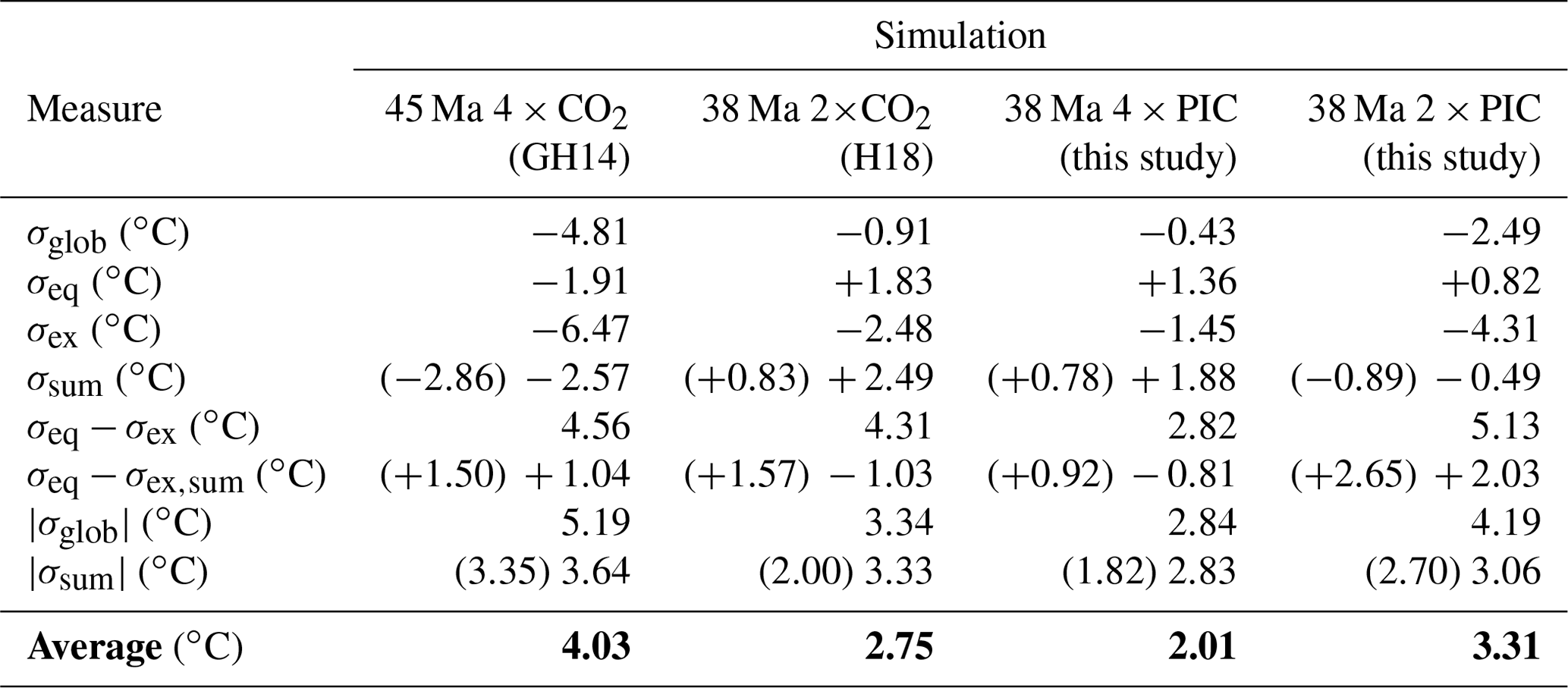
An overview of model skill scores is given in Table 4, comparing modelled SSTs from the 45 Ma 4 × CO₂ (GH14), 38 Ma 800 ppm (2×) CO₂ (H18), and our 38 Ma 4 × PIC cases to 42–38 Ma proxies and those of our 38 Ma 2 × PIC to 38–34 Ma proxies. Although all of the considered model cases simulate on average cooler SSTs than those suggested by the proxies (σ_glob<0), considerable improvement is seen for the new 38 Ma cases (including H18). The Equator-to-pole temperature gradient is still being overestimated by the models, but the discrepancy (σ_eq−σ_ex) is smallest for the 38 Ma 4 × PIC case presented here. As expected, better model skill is seen when considering summertime temperatures but only if those are highly underestimated by the annual mean. This is thus not the case for our 38 Ma 4 × PIC and H18 800 ppm CO₂ results, as the improvement at some sites is compensated for by others at which the proxies better agree with annual mean SST (see also Figs. 6 and 7). Those two model cases even underestimate the meridional gradient, taking summertime temperatures at extra-tropical locations (dashed red line in the inset of Fig. 6). This indicates that we cannot simply assume either an overall summer bias in those proxies or a cold bias in the models at extra-tropical sites. Indeed, further improvement of the model–proxy agreement is seen when considering modelled summer temperatures only at those sites where they provide a better match to the corresponding proxy estimate. For nearly all of the respective skill measures the 38 Ma 4 × PIC results show the best agreement with the available 42–38 Ma SST proxies, followed closely by those of H18 at 800 ppm CO₂.

Table 4Model skill scores following a procedure comparable to the one presented by Lunt et al. (2012) for the model results of GH14, H18, and those presented here using the 42–38 Ma SST proxy compilation from Fig. 6 (see also Table S3). The last column considers the 38 Ma 2 × PIC case and 38–34 Ma SST proxies (see Fig. S10 and Table S4). Different measures are used (top to bottom): global, equatorial (<23.5^∘ N or S), extra-tropical (>23.5^∘ N or S), summer temperatures (only for >23.5^∘ N or S), meridional temperature gradient (i.e. equatorial and extra-tropical; annual or summer), global absolute error, and summer absolute error. Bracketed values indicate model skill using modelled summer temperatures only when they improve agreement with the corresponding proxy estimate. An average skill score for each model–proxy comparison is also determined by taking the root mean square of all the above measures and highlighted in bold.

Download Print Version | Download XLSX

3.4 Climate sensitivity of the middle to late Eocene

The difference in the global average equilibrium temperature between our 38 Ma 2 × PIC and 4 × PIC simulations (3.21 ^∘C; see Table ) is similar to the model's response to a CO₂ doubling in the pre-industrial reference (3.14 ^∘C). Yet, the estimated radiative forcing from a second PIC doubling (ΔRF${}_{\mathrm{2}\times }^{\mathrm{4}\times }=\mathrm{5.15}$ W m⁻²) results in a considerably lower equilibrium climate sensitivity for our Eocene simulations: S_EO=0.62 ^∘C W⁻¹ m². Even in this virtually ice-free world significant polar amplification is found in the warming response to a PIC doubling, which ranges between 2 ^∘C in low-latitude regions to as much as 8 ^∘C at high latitudes (∼0.4–1.6 ^∘C W⁻¹ m²; see Fig. 9a–b). Zonal variation in the warming signal is highest at middle latitudes because of land–ocean contrasts, while differences in seasonal response are largest in polar regions. The polar amplification is reflected by differences in outgoing longwave radiation, being increasingly positive towards higher latitudes as a result of the Planck feedback (Fig. 9c–d). Overall net negative longwave fluxes over equatorial regions can be explained by tropopause responses and stratospheric cooling, which reduce outgoing radiation. On a more regional scale, alternating signals of differences in shortwave and longwave radiation occur with a pronounced minimum at the Equator and maxima over the ITCZ locations. This suggests the importance of cloud cover, which is seen to differ substantially (Fig. 9e–f) between the 38 Ma 2 × PIC and 4 × PIC cases. An increase in deep convective clouds over the equatorial Pacific corresponds to lower fluxes (more reflection of incoming shortwave and less outgoing longwave), while the opposite is seen off the Equator. Differences in cloud cover are seen to have a warming effect over most of the high-latitude regions. Increased wintertime low cloud cover over Antarctica and reduced summertime low cloud cover over the Arctic, along with increased high cloud cover, tend to warm the surface. The overall slight net heat loss (shortwave < longwave difference) at low latitudes versus a gain at middle to high latitudes agrees with a reduced meridional heat transport seen in the warmer 4 × PIC climate (Fig. 5c, d).

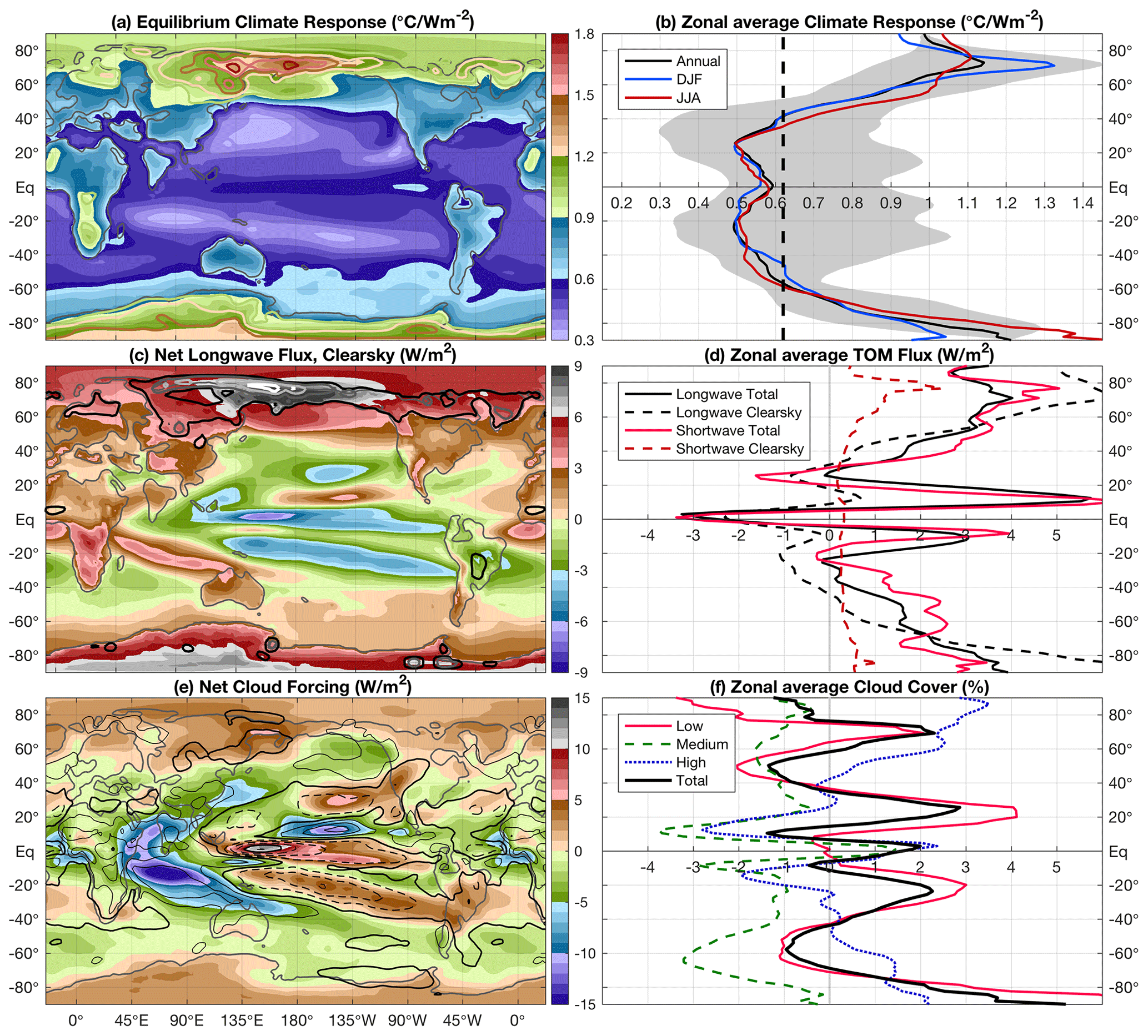
Figure 9(a) Annual mean temperature response, normalised by the global average TOM forcing (in W m⁻²) of the 38 Ma 4 × PIC compared to the 2 × PIC equilibrium climate with contours showing the winter season only (using the same colour scale). (b) Zonal average normalised temperature response; annual (black, shading for zonal variation), December–January–February (blue) and June–July–August (red). The (area-weighted) global average response (i.e. climate sensitivity) is 0.62 ^∘C W⁻¹ m² as indicated by the black dashed line. (c) Clear-sky component of the net longwave flux change at the TOM for 38 Ma 4 × PIC vs. 2 × PIC, similar for the clear-sky shortwave flux in contours (black to white; 1, 2, 5, and 10 W m⁻²). (d) Zonal average TOM flux change for longwave (black) and shortwave (red) fluxes, corresponding clear-sky components are shown using dashed lines. Note that longwave fluxes are defined positive upward while shortwave fluxes are positive downward. (e) Change in the total cloud forcing; longwave component (shading) and shortwave (contours every 5 W m⁻²; solid positive and dashed negative, thick black line at 0 W m⁻²). (f) Zonal average changes in cloud cover (in %) at low (solid red), medium (dashed green), high (dotted blue) and all (thick solid black) atmospheric levels.

As in the present-day climate the polar amplification is due in part to albedo effects from clouds, vegetation, snow cover, and some seasonal sea ice, but it is also the result of a strong water vapour feedback and meridionally dependent lapse-rate feedback (less negative towards higher latitudes). Low-latitude regions generally warm less than the global average in response to a positive radiative forcing, as they are strongly governed by moist processes (i.e. cloud cover and negative lapse-rate feedback) and more tied to SSTs (low land fraction). Additionally, the total column water vapour induces a negative shortwave feedback that is strongest in the tropics and helps to explain the smaller warming between our 38 Ma 2 × PIC and 4 × PIC than would be expected based on radiative forcing alone. An overview of zonally averaged atmospheric temperature changes between some of the different model cases considered here can be found in Fig. S15.

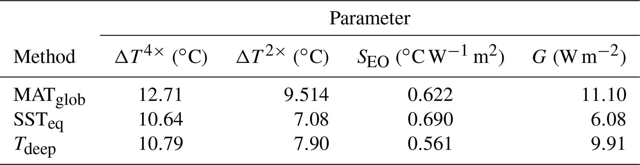
A list of averaged differences in our 38 Ma 4 × PIC and 2 × PIC simulations with respect to the pre-industrial reference is presented in Table 5, considering global near-surface air temperature (MAT_glob), equatorial SST (SST_eq), and deep-ocean temperature (T_deep). Using Eq. (2), we can determine both the climate sensitivity S and integral geography effect G for the different measures. Not surprisingly, using MAT_glob yields the same value of S_EO=0.62 ^∘C W⁻¹ m², with G=11.07W m⁻² (so G∼6.89 ^∘C). The estimate of G decreases when using only oceanic temperatures as the direct effect of cooler temperatures over pre-industrial land ice is removed. While considering global MAT differences will likely overestimate the effect of global geography changes (mainly through lapse-rate effects on ice sheets and mountains), the opposite is true for equatorial SSTs. The corresponding results for S_EO show less variation between different methods as they are tied to the respective temperature changes between the 38 Ma 2 × PIC and 4 × PIC cases. A possible range of G=6.08–11.10 W m⁻² is found, equivalent to ∼1.6–2.6 CO₂ doublings or a 4.2–6.9 ^∘C warming globally.

Table 5Temperature differences comparing the 38 Ma 4 × PIC (ΔT^4×) and 2 × PIC (ΔT^2×) Eocene climate to the pre-industrial reference as well as derived values for equilibrium climate sensitivity (S) and forcing from (integral) geography changes (G) using Eq. (2). Results are shown using global average 2 m temperature, equatorial SST (with a 3∕2 ratio, as discussed in Royer et al., 2012), and deep-sea temperature (below 2 km).

Download Print Version | Download XLSX

A more direct estimate of G can be obtained by comparing a pre-industrial climate under 2 × PIC and 4 × PIC with the results from the modelled 38 Ma 2 × PIC case. Using the model's pre-industrial ECS (S_PI=0.80 ^∘C W⁻¹ m²) and radiative forcing of two consecutive PIC doublings (ΔRF^2× and ΔRF^4×) yields an expected warming of 3.34 ^∘C and 7.46 ^∘C, respectively. As the modelled change in global average temperature with respect to the pre-industrial reference is either 9.50 ^∘C (2 × PIC) or 12.71 ^∘C (4 × PIC), an additional warming of 5.25–6.16 ^∘C takes place owing to integrated global geography changes (the effect of which is thus not entirely independent of the climatic state).

A similar exercise can be done for all of the different cases shown in Fig. 10 using S_EO on one hand and S_PI in combination with the previously defined values of RF and the available model results on the other hand. The projected temperatures suggest a contribution of ∼10 % at 2×CO₂ ∕ PIC and ∼20 % at 4 × CO₂ ∕ PIC from slow feedbacks (e.g. deep ocean, water vapour) to the global average warming response. The respective equilibrium temperatures for either pre-industrial or Eocene climates then yield a consistent estimate of G=8.6 W m⁻², corresponding to a 5.3–6.9 ^∘C global average temperature difference.

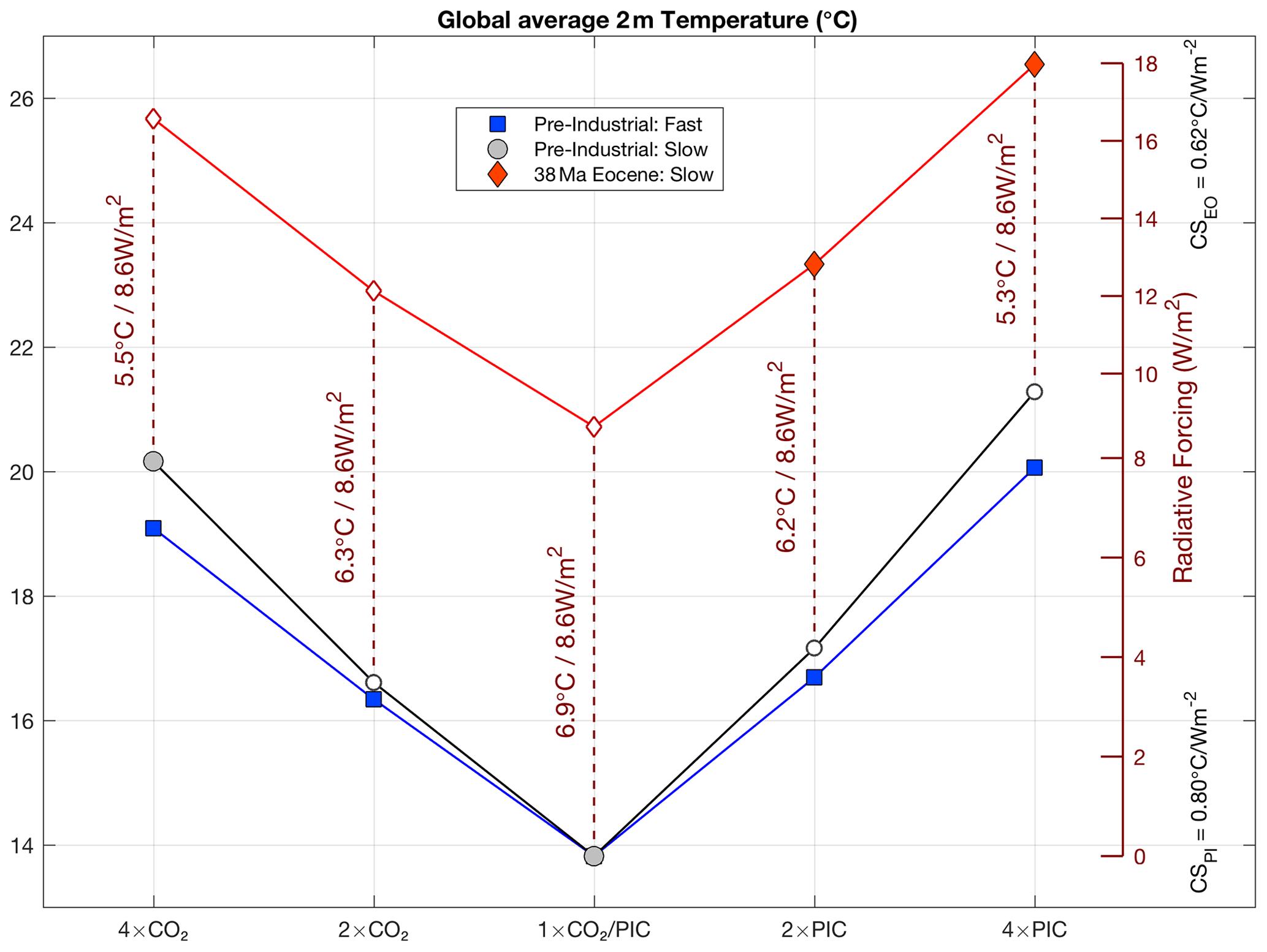
Figure 10Overview of globally averaged near-surface air temperatures in the different pre-industrial reference (blue) and 38 Ma Eocene (red) simulations. Blue squares show the extrapolated temperature response of fast feedbacks from 20-year perturbations (4 × CO₂, 2×CO₂, 2 × PIC, and 4 × PIC), while grey circles also include that of slow feedbacks. Filled markers indicate results from equilibrated simulations, and open markers show values that were estimated from the model-derived climate sensitivity and radiative forcing (red axis to the right; note the change in scale between pre-industrial and Eocene using S_PI and S_EO, respectively). Offsets in both temperature and radiative forcing (i.e. G) between pre-industrial and 38 Ma Eocene cases are specified for all of the considered atmospheric compositions.

Download

The possible range of G obtained here (∼6–11 W m⁻²; 4–7 ^∘C) is considerably higher than either the estimated 1.8 ^∘C warming related to geography (using HadCM3L) found by Lunt et al. (2012) or the ∼2–4 W m⁻² (i.e. 0.6–1.1 CO₂ doublings) suggested by Royer et al. (2012). A comparably high warming of ∼5 ^∘C from integral geography effects in the Eocene was proposed by Caballero and Huber (2013) and was found more recently for the early Eocene by Zhu et al. (2019). Higher estimates of 2–6 ^∘C can also be deduced using the different models considered by Lunt et al. (2012).