

Abstract
Extensive least-squares wavelet and cross-wavelet analyses are performed on the Very Long Baseline Interferometry (VLBI) baseline length and temperature time series for a network of four VLBI antennas located in different continents. These analyses do not rely on any pre-processing of the measurements including interpolations or gap-filling, and they can provide accurate instantaneous frequency information along with phase differences in the time–frequency domain. Out of four antennas mounted in Fortaleza, Hartebeesthoek, Westford, and Wettzell, the most and the least possibly impacted VLBI time series by the annual temperature variation are Westford–Wettzell and Fortaleza–Hartebeesthoek, respectively. Furthermore, the annual components of the temperature time series in Westford and Wettzell lead the ones in the corresponding VLBI time series by nearly one month, where one of the baseline sides is either in Westford or Wettzell.
Export citation and abstract BibTeX RIS
1. Introduction
Geodetic Very Long Baseline Interferometry (VLBI) is a geometric technique that uses radio telescopes to estimate the distance between the telescopes and to determine the Earth orientation parameters (Schuh & Behrend 2012). The distance between two radio telescopes, known as the baseline length, is calculated from the time difference between the arrivals of the radio signals emitted from an astronomical radio source, such as a quasar (Sovers et al. 1998).
A VLBI baseline length time series is obtained by recording measurements over time. The VLBI time series are unequally spaced (unevenly sampled) and have uncertainties (error bars) due to several reasons including atmospheric conditions, maintenance of the radio telescopes, and economy. Errors in measurements, caused by the ionosphere and troposphere, deformations of the Earth's crust and unreliability of the receivers and stations clocks, have been minimized during the last three decades, and recently the baseline length measurements have an accuracy of a few millimeters (Boehm et al. 2009, 2018; Heinkelmann et al. 2011). One of the main sources of the remaining errors is due to the temperature variations that can deform the structure of the antennas and affect the measurements (Wresnik et al. 2007). Neglecting atmospheric pressure and hydrological loading corrections at the observation level can also contaminate the time series by introducing annual and seasonal signals, like in Global Navigation Satellite System time series (Rabbel & Schuh 1986; Vandam et al. 1994; Zou et al. 2015).
The main goal of this research is to show the potential of the Least-Squares Wavelet (LSWAVE) software 1 (Ghaderpour & Pagiatakis 2019) for analyzing VLBI time series and coherency analyses. For the latter, it is shown how the temperature variations may possibly change the VLBI measurements with the main focus on the annual variations. The results also suggest how one can improve the estimation of the gradual change in the baseline length by not simply using a traditional regression analysis.
2. Materials and Methods
2.1. Materials
2.1.1. Study Sites
Various factors may indirectly impact the VLBI baseline length including structures and materials of the VLBI antennas, global station position, and climatology effects (Wresnik et al. 2007). To investigate the possible effect of temperature variations on the baseline length, four stations are selected in different continents. They are located in Fortaleza (Ceara, Brazil—tropical zone), Hartebeesthoek (Gauteng, South Africa—subtropical zone), Westford (Massachusetts, USA—temperate zone), and Wettzell (Bavaria, Germany—temperate zone), see Figure 1. The diameters of the parabolic antennas in Fortaleza, Hartebeesthoek, Westford, and Wettzell are 14.2 m, 26 m, 18.3 m, and 20 m, respectively. The VLBI antenna in Westford is housed under a 28 m radome formed by an inflated fabric-reinforced teflon sheet to withstand wind speeds of up to 160 km hr−1.
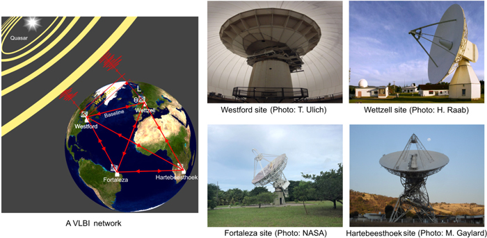
Figure 1. A VLBI network with four radio telescopes. Arrows in the left panel show the direction of displacement. Distance L is estimated from the time difference between identical radio signals arriving at the two antennas multiplied by the speed of light. The baseline length can be estimated from the orientation angle θ and distance L.
Download figure:
Standard image High-resolution image2.1.2. Data Sets and Pre-processing
The VLBI baseline length time series are downloaded from the International VLBI Service for geodesy and astrometry (IVS) combination center 2 . The time unit of the time series is the modified Julian date. Table 1 shows more details of these unequally spaced time series whose measurements (24 hr long observing sessions) are associated with standard deviations (error bars). The baseline data were analyzed during the combination process, and so the same epoch and equal constraints were used for each session (Bachmann et al. 2015, 2016).
Table 1. Duration and Size of the VLBI Baseline Length Time Series Used Herein
| VLBI Baseline Sites | Start Date | End Date | Series Size |
|---|---|---|---|
| Fortaleza–Hartebeesthoek | 1993 Jul 13 | 2018 Apr 12 | 345 |
| Fortaleza–Westford | 1993 Jul 13 | 2014 Aug 27 | 332 |
| Hartebeesthoek–Westford | 1986 Feb 4 | 2014 Sep 4 | 568 |
| Westford–Wettzell | 1984 Feb 24 | 2014 Sep 4 | 1380 |
| Fortaleza–Wettzell | 1993 Jul 7 | 2019 Sep 27 | 1558 |
| Hartebeesthoek–Wettzell | 1986 Feb 4 | 2018 Sep 13 | 661 |
Note. The end date is when the last measurement was estimated to date. Size also refers to the number of sessions, where each session provides one baseline length measurement.
Download table as: ASCIITypeset image
The temperature data sets for each site are downloaded from the Vienna mapping functions website 3 (Boehm et al. 2006). The average and standard deviation of temperature data for each day are calculated to obtain a daily temperature time series for each site as the main focus herein is the study of the annual variations.
2.2. Methods
2.2.1. The Least-squares Spectral Analysis
The Least-Squares Spectral Analysis (LSSA) is a robust method of estimating a frequency spectrum for a given time series (Vaníček 1969; Lomb 1976). In LSSA, the time series does not have to be equally spaced and can also contain trends and/or datum shifts. LSSA also considers the covariance matrix associated with the time series that is usually a diagonal matrix containing the variances of the measurements. Considering the effect of removing the estimated constituents of known forms, such as trends, a normalized spectrum will be obtained by fitting the sinusoidal waves of a particular frequency to the residual series. The normalized spectrum, namely, the Least-Squares Spectrum (LSS) shows how much the sinusoids of a particular frequency contribute to the residual time series.
Regarding the statistical properties of LSSA, in practice, when the time series has been derived from a population of normally distributed random variables, LSS follows the beta distribution. Thus, a spectral peak in LSS will be statistically significant at a certain confidence level if its value, usually expressed as a percentage variance, becomes larger than the critical percentage variance (Pagiatakis 1999).
For an unequally spaced time series, LSSA may not accurately estimate the signals even if a denser set of frequencies are examined. One of the main reasons is that LSSA ignores the correlation among the sinusoidal waves of different frequencies, causing spectral leakages in LSS (Ghaderpour 2018). To attenuate the leakages and estimating the signals more accurately, Ghaderpour et al. (2018b) proposed an iterative algorithm, namely, the Anti-Leakage Least-Squares Spectral Analysis (ALLSSA), that finds an optimal set of sinusoidal waves along with the constituents of known forms that simultaneously fit best to the time series.
2.2.2. The Least-squares Wavelet Analysis
Decomposing a time series with unstable components over time into the frequency domain can be misleading. For instance, a spectral peak in LSS does not show whether the peak corresponds to a short-duration wave with large amplitude or a long-duration wave with a small amplitude. To address this issue, Ghaderpour & Pagiatakis (2017) proposed the Least-Squares Wavelet Analysis (LSWA) that decomposes a time series into the time–frequency domain using an appropriate windowing technique to obtain a Least-Squares Wavelet Spectrogram (LSWS). The window size in LSWA is inversely proportional to the frequency which means as frequency increases the segment size decreases and vice versa, allowing the detection of short- and long-duration signals. LSWA is a natural extension of LSSA that can show how the signal amplitude and the percentage variance of its corresponding peaks change over time (Ghaderpour & Ghaderpour 2020).
The covariance matrix associated with the time series is also considered in LSWA to define appropriate statistical weights that can potentially improve the detection of signals from the noisy measurements. Furthermore, a Gaussian function can be applied to adapt the sinusoidal basis functions to the Morlet wavelet within each translating window in the least-squares sense (Foster 1996; Ghaderpour & Pagiatakis 2017). A stochastic confidence level surface can also be defined from the principals of LSSA to show whether the spectral peaks in LSWS are statistically significant at a certain confidence level (usually 95% or 99%). In other words, if a peak stands above the stochastic surface, then it is statistically significant (Ghaderpour 2018).
2.2.3. The Least-squares Cross-wavelet Analysis
Coherency analysis is a powerful approach for investigating the impact of one phenomenon on another in the frequency or time–frequency domain, e.g., investigating the influence of temperature or precipitation variations on plant phenology (Ghaderpour & Vujadinovic 2020). The Least-Squares Cross-Wavelet Analysis (LSCWA) simply multiplies the LSWSs of two time series obtained for a given time interval (Ghaderpour et al. 2018a). LSCWA has the following advantages over the popular cross-wavelet transform (XWT) (Torrence & Compo 1998):
- 1.The two time series do not have to be equally spaced, and they can have different sampling rates.
- 2.LSCWA considers the covariance matrices associated with the time series that can significantly reduce the effect of measurements with higher uncertainties.
- 3.LSCWA has a higher time–frequency resolution compared to XWT mainly because the correlations between the sinusoids are considered.
- 4.The constituents of known forms can be removed from the time series segments while the removal effects are considered in the residual series.
LSCWA also provides the phase differences between the components of interest in both time series, usually displayed by arrows in the Least-Squares Cross-Wavelet Spectrogram (LSCWS). The arrows follow the trigonometric circle principle in the two-dimensional Cartesian coordinate system. For example, if an arrow points to the right (toward the positive x-axis) for a peak in LSCWS, then the corresponding components of both time series have the same phase. Also, if the arrow is in the fourth quadrant with an angle ψ from the positive x-axis, then the component of the second time series leads the one in the first time series by ψ, i.e., the wave in the second time series reaches its maximum before the wave in the first time series, having the phase difference ψ which can be converted to time with respect to the signal frequency (Ghaderpour 2018; Ghaderpour & Vujadinovic 2020).
The Least-Squares Cross-Spectral Analysis (LSCSA) is a special case of LSCWA that obtains a Least-Squares Cross-Spectrum (LSCS) by multiplying the LSSs of the two series, i.e., LSCS shows the coherency in the frequency domain rather than in the time–frequency domain (Ghaderpour 2018). Ghaderpour et al. (2018a) also derived the stochastic confidence level surfaces in LSCWA when the two time series are assumed to be derived from two populations of statistically independent random variables following the multi-dimensional normal distributions, likewise for LSCSA.
3. Results and Discussion
3.1. LSSA, ALLSSA, and LSWA Results
Herein, due to the main focus on annual changes and coarsely sampled VLBI series, maximum cyclic frequency is chosen to be six cycles per year (c/a) to avoid possible aliasing as the Nyquist frequency is not well defined for unequally spaced time series (Craymer 1998; VanderPlas 2018). Also, since the overall baseline length evolution changes almost linearly, the linear trend is selected as the constituent of known form for all the time series (Ghaderpour & Pagiatakis 2017).
The six VLBI baseline length time series along with their error bars are illustrated in Figure 2. Figure 3 shows LSSs and LSWSs of the VLBI series. For a better visualization, the ALLSSA estimated linear trends, shown in Figure 2, are subtracted from the time series. The least and the most significant annual variations are for Fortaleza–Hartebeesthoek and Westford–Wettzell, respectively, see the horizontal band of spectral peaks with percentage variance greater than 30% at 1 c/a in LSWS of panel (d) and compare them with other panels. Furthermore, inter-annual peaks (<1 c/a) are also observed in all LSSs and LSWSs as well as intra-annual short duration peaks (>1 c/a). Figure 4 demonstrates the temperature time series for the four sites along with their LSSs and LSWS. The Westford site has the most significant annual temperature variation (≈80%) followed by Wettzell (≈50%) and Hartebeesthoek (≈30%).
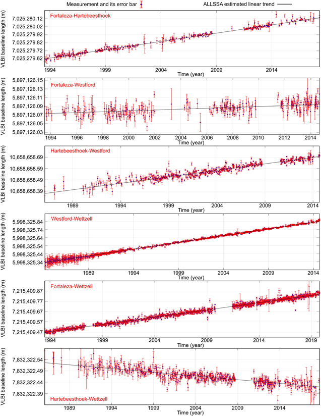
Figure 2. The VLBI baseline length time series along with their ALLSSA estimated linear trends whose intercepts and slopes are listed in Table 2.
Download figure:
Standard image High-resolution image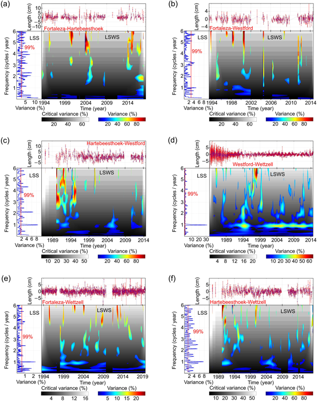
Figure 3. The spectra and spectrograms of the VLBI baseline length time series. To visualize the oscillations better, the de-trended time series are shown here. The gray surface is the stochastic surface at 99% confidence level.
Download figure:
Standard image High-resolution image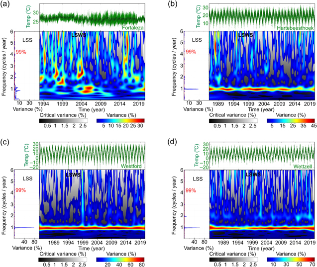
Figure 4. The spectra and spectrograms of the daily temperature time series shown along with their error bars. The gray surface is the stochastic surface at 99% confidence level.
Download figure:
Standard image High-resolution imageThe ALLSSA simultaneously estimated annual amplitudes, intercepts and slopes of the linear trends for the VLBI and temperature time series are listed in Table 2. The estimated linear trends for the VLBI baseline length time series are shown in Figure 2. Note that several inter-annual and intra-annual components are also simultaneously estimated by ALLSSA for these time series but are not listed in Table 2 for brevity. The maximum displacement rate of 16.79 millimeter per year (mm/a) in this network is for Westford–Wettzell, and the minimum is for Fortaleza–Westford with a rate of approximately 1 mm/a.
Table 2. The ALLSSA Estimated Intercepts and Slopes of the Linear Trends, and Amplitudes of the Annual Components of the VLBI Baseline Length and Temperature Time Series
| VLBI Baseline Sites | Intercept (m) | Slope (mm/a) | Amplitude (mm) |
|---|---|---|---|
| Fortaleza–Hartebeesthoek | 7025, 279.6195 ± 0.0016 | 20.66 ± 0.10 | None |
| Fortaleza–Westford | 5897, 126.0699 ± 0.0015 | 1.00 ± 0.10 | 2.76 ± 0.71 |
| Hartebeesthoek–Westford | 10,658, 658.3683 ± 0.0030 | 11.45 ± 0.14 | 6.41 ± 0.82 |
| Westford–Wettzell | 5998, 325.3282 ± 0.0005 | 16.79 ± 0.02 | 4.21 ± 0.18 |
| Fortaleza–Wettzell | 7215, 409.4627 ± 0.0006 | 14.18 ± 0.04 | 3.09 ± 0.42 |
| Hartebeesthoek–Wettzell | 7832, 322.5256 ± 0.0019 | −3.31 ± 0.10 | 4.85 ± 0.59 |
| Temperature Sites | Intercept (°C) | Slope (°C/a) | Amplitude (°C) |
| Fortaleza | 26.86 ± 0.02 | −0.038 ± 0.001 | 0.20 ± 0.01 |
| Hartebeesthoek | 17.72 ± 0.05 | 0.006 ± 0.003 | 3.11 ± 0.04 |
| Westford | 10.52 ± 0.07 | 0.004 ± 0.003 | 11.33 ± 0.05 |
| Wettzell | 7.37 ± 0.07 | 0.026 ± 0.003 | 8.38 ± 0.06 |
Note. The VLBI trend intercepts are the y-axis values (baseline lengths) at the start times listed in Table 1. Also, the temperature trend intercepts are the y-axis values at the beginning of Januaries of 1993, 1986, 1984, 1984 for Fortaleza, Hartebeesthoek, Westford, and Wettzell, respectively.
Download table as: ASCIITypeset image
3.2. LSCSA and LSCWA Results
First, to visualize the annual pattern of temperature for each site, the average monthly temperatures are calculated since Januaries of 1993, 1986, 1984, 1984 for Fortaleza, Hartebeesthoek, Westford, and Wettzell, respectively, and the results are illustrated in Figure 5. The most and the least annual temperature variations are observed in Westford and Fortaleza, respectively. The maximum monthly temperatures are in July for Westford and Wettzell, while the minimum temperature for Hartebeesthoek is in July. More precisely, the annual phase difference between Westford and Hartebeesthoek is about 161 days, and it is about 170 days between Wettzell and Hartebeesthoek from LSCSA.
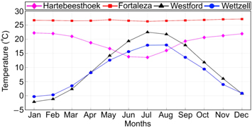
Figure 5. The average monthly temperatures of the four study sites.
Download figure:
Standard image High-resolution imageThe interpretation of the coherency analysis results presented in this section is based on the assumption that temperature variations can affect the baseline length measurements. Note that temperature is not the only factor impacting the measurements. Figures 6 and 7 show LSCSs and LSCWSs of the VLBI and temperature series. The possible effect of temperature variations on the baseline length can be observed from the cross-spectrograms. Figures 6(a)–(b) show insignificant impact of temperature variations in Fortaleza and Hartebeesthoek on the VLBI baseline length, see the small percentage variances corresponding to the annual coherency. On the other hand, Figures 7(a)–(b) show the most significant impact of temperature variations in Westford and Wettzell on the VLBI baseline length, see the large percentage variances corresponding to the annual coherency. This strong coherency is not observed for other baselines as Fortaleza and Hartebeesthoek are in the tropical and subtropical zones, respectively.
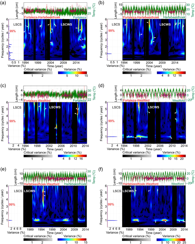
Figure 6. The cross-spectra and cross-spectrograms of the VLBI baseline length and daily temperature time series for the study sites. To visualize the oscillations better, the de-trended VLBI baseline length series are shown here. The gray surface is the stochastic surface at 99% confidence level. The phase differences between the components of both series are displayed by white arrows following the trigonometric circle principle, i.e., arrows pointing to the right, left, up, and down means, in-phase, out-of-phase, VLBI leads, and temperature leads, respectively.
Download figure:
Standard image High-resolution image
Figure 7. The cross-spectra and cross-spectrograms of the VLBI baseline length and daily temperature time series for the study sites. See the caption of Figure 6 for more details.
Download figure:
Standard image High-resolution image
For better visualization, the phase differences are shown by white arrows whose tails are located at the most significant spectral peaks where the percentage variances are the highest around small neighborhoods in the time–frequency domain. The direction of arrows on the annual coherent peaks in Figures 7(a)–(b) indicates that the annual components of temperature series in both Westford and Wettzell lead the ones in the VLBI series by a few weeks (Ghaderpour et al. 2018a). This possibly indicates that when the temperature reaches its minimum during winter, a few weeks after the annual component of the VLBI series reaches its minimum because the deformation of the antennas takes some time to shrink the baseline indirectly. The almost continuous significant band of coherent peaks for Westford–Wettzell may also be justified as the large annual amplitudes of temperatures in both Westford and Wettzell that are also almost in-phase, i.e., the annual phase difference is about nine days. The Root Mean Square (rms) of the first five years (1984–1989) of the de-trended VLBI baseline length series for Westford–Wettzell is 0.016 m that is about twice greater than rms of the rest of the series from 1989 to 2015. Whereas the annual temperature variations can be seen in the spectrograms of Figures 4(c)–(d) during 1984–1989, the insignificant annual coherency during this period as seen in the cross-spectrograms of Figures 7(a)–(b) may be explained by the noisy measurements in the earlier stage of VLBI operation, obscuring annual signals caused by temperature influence, see Figure 3(d).
Figure 4(b) shows an almost continuous horizontal band of annual peaks in the spectrogram, however, neither of the spectrograms in Figures 3(c) and (f) shows such a continuous annual band, i.e., the most statistically significant VLBI annual peaks are for years 1992 and 2005. From the cross-spectrograms shown in Figures 6(e)–(f) and 7(e)–(f), the insignificant annual coherency may possibly be due to the opposing climate seasons, see the direction of arrows. Overall, the directions of the arrows in all the cross-spectrograms shown in Figures 6 and 7 appear to be random except for the ones corresponding to the annual peaks, especially for Westford–Wettzell shown in Figures 7(a)–(b).
4. Conclusions
The spectral and wavelet analyses techniques used herein revealed inter-annual and intra-annual components in the six VLBI baseline length time series. A possible source of these wave-like variations is investigated by performing the coherency analysis with temperature time series corresponding to the four sites. The cross-spectrograms clearly showed that the most and the least significant annual coherency are for Westford–Wettzell and Fortaleza–Hartebeesthoek, respectively. All the analyses performed herein did not require any interpolation and gap-filling, and the error bars associated with measurements were considered, signifying the robust performance of the LSWAVE software. In the results presented herein, the measurements with relatively higher uncertainties (error bars) contributed relatively less to estimating time series components. Therefore, the noisy VLBI data at the early years of the experiment, particularly for Westford–Wettzell, did not play a significant role in estimating the trends and spectra. Investigating the impact of other phenomena, such as pressure, water vapor pressure, and wind on the baseline length are also interesting, and it is subject to future work.
The author would like to thank the scientists and personnel in the IVS combination center and the Department of Geodesy and Geoinformation of TU Wien and others for providing the data sets used in this research. The author also thank Dr. Harald Schuh and the anonymous reviewer for their comments that significantly improved the presentation of the paper.
Footnotes
- 1
Freely available online at: https://geodesy.noaa.gov/gps-toolbox/LSWAVE.htm and https://github.com/Ghaderpour/LSWAVE-SignalProcessing.
- 2
IVS combination center: https://ccivs.bkg.bund.de/, quarterly data by the Deutsches Geodätisches Forschungsinstitut (DGFI).
- 3
Vienna mapping functions website: https://vmf.geo.tuwien.ac.at/.