Instrumental Variable Analysis in Atmospheric and Aerosol Chemistry

Introduction

Instrumental variable analysis (IVA) has been utilized for understanding the causal effect of election day precipitation on electoral outcomes affecting the voters' decisions differently (Lind, 2020). IVA has also been utilized in “remote sensing” e.g., in estimating error of a geophysical product (Dong et al., 2019). IVA approach has been utilized too in “epidemiology” e.g., to provide the effectiveness of a high-dose over a standard-dose in protecting against influenza/pneumonia associated hospitalization, cardiorespiratory-associated hospitalization, and all-cause hospitalization, among others (Young-Xu et al., 2019). IVA has also been applied in the field of social science and statistics e.g., utilization of genetic markers as IV for assessing the effect of the risk factor on the outcome (von Hinke et al., 2016). However, to the best of our knowledge the application of IVA has not been done so far to assess feasibility of chemical transformations occurring in the atmosphere through gas-phase or multi-phase reactions. There are myriads of organic and inorganic compounds in the gas-phase in the ambient atmosphere (Zhang et al., 2019). Some of those compounds undergo chemical transformation owing to their reactivity with atmospheric oxidants/reactants (O₃, H₂O₂, NO_x, and OH radical) and may undergo a phase-change [e.g., secondary organic aerosol (SOA) formation] (Sato et al., 2013; Edwards et al., 2017). The chemical reactivity of a reactant and the formation of product/s both are influenced by several factors called confounders e.g., relative humidity (RH), temperature (T), and solar flux (SF), among others. Having measured a SOA species and an oxidant (per say O₃), if one attempts to find out the relationship between the two through regression analysis then the regression parameters will not be representative of the only effect of O₃ on SOA as there could also be the effect of confounders and other oxidants too. Thus, measuring reactants and products and simply relating the two does not mimic the actual effect of the reactant on the product. This drawback arises because of not achieving the randomization. The randomization makes exposure (here reactants) independent of measured/unmeasured confounders (here RH, T, SF). This can be achieved by different causal modeling approaches, one of which is the IVA (Hernán and Robins, 2020).

Broadly, there are two methods of causal modeling (Hernán and Robins, 2020). The first one is called propensity score methods that use the statistical analytics tool to make exposure independent of confounders (i.e., exchangeable). Another method uses quasi-experimental designs to achieve the exchangeability. While the propensity score method can control for measured confounders and rely on the assumption of no unmeasured confounders (are the ones that affect both exposure and the outcome, please refer to Figure 1), and no missing interaction terms, the quasi-experimental designs (e.g., IVA) can also control for unmeasured confounders, and rely on the assumption that the randomization created by the design worked. The propensity score (PS) is the predicted probability of exposure. Briefly, for a robust interpretation in the PS method one would need the data of all possible confounders to input into the model. PS calculation requires a set of methods to operate e.g., matching (nearest-neighbor matching, radius matching, and kernel matching), stratifying, adjusting for covariate in the regression model, and weighting. Finally, using the PS method the standardized mean differences are calculated for all variables that were input into the model (Schwartz et al., 2018). For continuous confounders the standardized mean difference is calculated as below:

And for dichotomous confounders, the standardized mean difference is calculated using the following equation:

Here, treatment and control groups represent reactive and non-reactive species. The “x_mean” and “â” represent the average of the data whereas “S” represents the standard deviation.

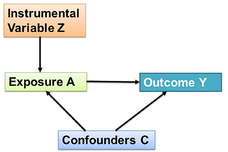
Figure 1. Directed Acyclic Graph (DAG) illustrating an instrumental variable Z.

For details on PS calculation, reference is made to Hernán and Robins (2020). The critical aspect of the propensity score method arises when there are unmeasured confounders. That is, if all the confounders are not inputted into the model then the PS method could underestimate/overestimate the effect of exposure on outcome. In quasi-experimental designs, there can be four different approaches: Instrumental Variable; Regression Discontinuity; Difference in Differences; and Natural Experiments (Hernán and Robins, 2020).

Briefly, the quasi-experimental designs seek to randomize exposure independent of confounders in different ways, which are not statistical manipulations (Schwartz et al., 2017, 2018). For details of statistical method and quasi-experimental designs, reference is made to (Hernán and Robins, 2020). IVA exploits the presence of an additional variable in the data, called an instrumental variable to achieve randomization. The instrumental variable plays the role of the random assignment.

Theory of IVA

Let us consider a directed acyclic graph (DAG) illustrating the instrumental variable (Z) analysis approach (Figure 1). Let A be the exposure, C be the confounders, and Y be the outcome variable. It is important to mention here that the association between Z and outcome Y is not confounded by C (measured/unmeasured confounders). Thus, by calibrating the instrument Z to A, the causal effect estimate of per unit increase in A on Y can be determined using regression analysis. To understand these terms in the context of aerosol chemistry an example could be given by considering exposure (A) by O₃, confounders (C) by relative humidity (RH), temperature (T), and solar flux (SF), the instrumental variable (Z) by BLH or wind speed, and the outcome (Y) by the SOA fraction.

Now, we shall discuss the mathematical perspectives of IVA. Let ${\text{Y}}_{\text{t}}^{\text{A}=\text{a}}$, ${\text{Y}}_{\text{t}}^{\text{A}=\text{a}}$' be the potential outcomes at observation t under the exposures a and a'. Now, if Y^{A = a} ≠ Y^{A = a}' then it is inferred that A has a causal effect on Y. The causal estimates can be represented mathematically by two parameters as below:

Summing up, under two different exposure conditions if we get different outcomes then there is a causal effect of exposure on the outcome.

Let us suppose that the outcome depends on predictors in the following manner:

Where η_t represents the impact of all other variables on the outcome, ϕ₀ is intercept, and ϕ is the coefficient of A_t.

Suppose we have a variable Z such that Z is associated with Y only through A. Its association with A can be expressed as:

Where, τ_t represents the variations in exposure that are associated with other predictors of outcome, measured or unmeasured and σ is the coefficient of Z_t. Z_tσ is the variation in exposure due to the instrument, and hence independent (by assumption) of confounders.

Let Z1 be the Z such that:

and similarly,

Here, E(A|Z1) = a represents that the expected value of exposure variable A at Z = Z1 is a, and E(A|Z2) = a' represents that the expected value of exposure variable A at Z = Z2 is a'.

From Equations 5 and 7, it can be derived that:

Similarly, from Equations 5 and 8, it can be derived that:

Subtracting Equation 10 from Equations 9 would yield:

Here, ϕ, which is a log rate ratio, is the causal effect of exposure on outcome in which we are interested.

Summing up, first regress exposure against the instrument and then regress the outcome against instrument to get the causal effect estimate. The ratio of the two coefficients is the causal effect of a unit change in exposure. The instrument Z should explain a part of the variation in A that is not confounded by other predictors of the outcome. It is worthwhile mentioning that in IVA the confounders (measured/unmeasured) do not play any role while estimating the effect of exposure on the outcome. This is one of the major advantages of IVA over other quasi-experimental designs as often we do not have the data set of all confounders in atmospheric and aerosol chemistry research.

Hypothesis, Randomization, and Good Instrument

Hypothesis Under Examination

While assessing the effect of O₃ on SOA formation (e.g., here, f_SOC = SOC/OC ratio), it would be important to notice the variability of f_SOC as a function of O₃. If the behavior of outcome (f_SOC) is linear to the predictor (O₃) then it is possible to build a linear regression model between the two as follows:

Here, β₀ is the intercept, β₁ is the slope, and ε is the residual. A normal-distribution is observed for residuals [ε ~ N (0, σ²)] in linear regression analysis (i.e., with a mean zero and variance σ²). The null and alternate hypotheses for the above linear regression model are given below:

Only if null hypothesis is rejected, we can get a causal estimate of O₃ on SOA formation. We seek the cases where the null hypothesis is rejected as it leads toward the causal effect estimate.

Randomized Experiments and Exchangeability

The major issue while inferring causality arises due to unmeasured parameters. Inferring causality for each data point means coming up with a valid surrogate for the unobserved counterfactual, which is hard to imagine. So, to infer causality, the randomization (exchangeability) experiment is conducted. The randomization process makes the exposure independent of confounders (measured/unmeasured). Achieving randomization means that the distribution of confounders is the same in unmeasured and measured data points. Statistically it can be understood by assuming that outcome (Y^{a = 1}) for the data point which happened to be measured is the same as outcome (Y^{a = 1}) for the data point which was not measured. After randomization, the Pr(Y = 1|A = 1) is a consistent estimate of Y^{a = 1} (where Pr is a conditional probability of outcome under A = 1). Thus, if the probability of the outcome [or E(Y)] among measured data points is the same as the probability [or E(Y)] among the entire population then the exposures are exchangeable. The exchangeability is achieved by random assignment. Exchangeability can be achieved in several ways, one of which is the IVA.

Good Instrument for a Valid IVA Inference

There are two essential requirements for IVA inference to be valid:

i. The instrument needs to explain enough variation of exposure variable A and its average causal effect on A should be non-zero.

ii. The instrument must not have a direct causal effect on outcome Y.

The most important question while performing IVA in atmospheric and aerosol chemistry is like what would be a good instrument to explain the chemical transformation in a study? For example suppose a research problem focuses on the formation of SOA through oxidation of VOCs under ambient atmospheric conditions. Furthermore, the researchers are interested in finding the effect of O₃ on the SOA formation estimate. This research problem seems to be confounded by the RH, T, and solar flux (for DAG refer to Figure 1). Having understood all these backgrounds if a good instrument can be found then IVA can be performed and the causal inference on SOA formation due to per unit change in O₃ can be determined as discussed above. For most of the atmospheric and aerosol chemistry problems, the authors encourage to utilize either boundary layer height (BLH, aka mixing height) or wind speed as an instrument. It is worthwhile mentioning that BLH and wind speed affect the concentration of pollutants, but will not change the relative abundance (ratio) of any two species (e.g., outcome here, f_SOC = SOC/OC). The validity of the results should be checked with p-value (level of significance) and model output confidence interval (CI: 95% or 99%). More importantly, the NULL hypothesis of a problem under the study must be checked with the CI values.

The validity of the instrument needs to be checked using the machine learning algorithm. The important caveat of IVA is that under some research problems the instrument predicts changes in a subset of exposure population. In these scenarios, the instrument will provide the average treatment effect for the subset of the data and not for the entire population. This is called the local average treatment effect. This must be investigated for the problem under investigation. For example, in atmospheric science it is likely that sometimes we may get an extremely high or a very low value of exposure variable (here, O₃). Then it is required to consider those extreme high/low data points as outliers and re-run the model for the output.

Application of IVA to the Field-Data

Methodology

Field-Campaign

A field campaign was conducted from 08th Nov 2015 (local time: 10:00 h) to 16th Nov 2015 (local time: 06: 00 h) at Kanpur location (26.30°N, 80.14°E, 142 m asl.), situated in central part of the Indo-Gangetic Plain (IGP). In this campaign, we have measured organic and elemental carbon (OC-EC), near ground-level O₃, and mass concentrations of PM_2.5. Briefly, the analytical instruments were housed in Atmospheric Particle Technology Laboratory (APTL, first floor, ~25 ft. above the ground level) at the Center for Environmental Science & Engineering (CESE) building in Indian Institute of Technology Kanpur (IITK) premises. The entire data set has been sub-divided into three periods: Pre-Diwali (08th to 10th Nov.), Diwali festival (11th Nov.), and Post-Diwali (12th to 16th Nov.). The OC-EC has been measured using a Sunset laboratory semi-continuous Carbon analyzer using NIOSH (National Institute for Occupational Safety and Health) protocol (Birch and Cary, 1996; Rajput et al., 2017). O₃ has been measured on an ozone analyzer (Thermo Scientific; Model # 49i) by UV-photometric technique. Particles number concentrations (PNC) were measured in the aerodynamic size-range of 0.25–2.5 microns on an Aerosol Spectrometer (PALAS, Germany). Assuming spherical shape and apparent density (1.1 g cm⁻³), the PNC (#/cm³) was converted into mass concentration (μg m⁻³) following the approach given in earlier publications (Pitz et al., 2003; Izhar et al., 2018; Rajput et al., 2019). These instruments were kept nearby on a platform in the lab, and their inlets (separated by <1 m) were drawing air from the ambient atmosphere through a window located in the rear-side of the CESE building. Details on instrumentation and analysis are given in the Supplementary Material.

In this study, the secondary organic carbon (SOC) was estimated by the minimum OC/EC ratio method using the below-given equations (Castro et al., 1999; Ram et al., 2008; Rajput et al., 2018).

Here, OC_prim refers to primary organic carbon whereas (OC/EC)_min refers to the minimum OC/EC ratio. The minimum OC/EC ratio was 3.2, 3.4, and 5.0 during Pre-Diwali, Diwali, and Post-Diwali periods, respectively. The SOC/OC ratio has been referred to as f_SOC (fraction of SOC in total OC) and POC/OC has been referred to as f_POC (fraction of POC in total OC) in the subsequent discussion.

Retrieval of the Meteorological Data Set

Meteorological parameters viz. ambient temperature (T), wind, and relative humidity (RH) have been retrieved from the on-campus weather station. Boundary layer height (BLH), solar flux (SF), and 5-days air-mass back trajectories (AMBTs, GDAS 0.5°, @ 1,000 m above ground level) data have been retrieved from NOAA HYSPLIT (Hybrid Single-Particle Lagrangian Integrated Trajectory) model (Draxler and Rolph, 2003; Stein et al., 2015). AMBTs have been coupled with PM_2.5 mass concentration data for cluster and concentration-weighted trajectory (CWT) analysis (discussed in the subsequent section).

Data Processing in R

Data analysis, statistical analysis, instrumental variable analysis (IVA), and machine learning coding have been carried out in R (Carslaw and Ropkins, 2012; Schwartz et al., 2017, 2018; Hernán and Robins, 2020).

Results and Discussion

Temporal Variability of PM_2.5, OC, EC, and OC/EC Ratio

During the entire campaign, we have observed a quite high variability in mass concentrations of PM_2.5, OC, EC, and OC/EC ratio (Figure 2). Overall, PM_2.5 concentrations varied from 128–901 μg m⁻³. The PM_2.5 concentrations averaged at 331 ± 48 μg m⁻³ (Avg. ± SD) during Pre-Diwali daytime period (08th−10th Nov) and looks statistically different as compared to that observed during Pre-Diwali nighttime period (Avg. ± SD = 272 ± 93 μg m⁻³; t-value = 22.6, Table 1). Similarly, the daytime (389 ± 157 μg m⁻³) and nighttime average values (443 ± 145 μg m⁻³) of PM_2.5 concentrations were also significantly different (t-value = 6.5) on Diwali festival event (11th Nov). Furthermore, during Post-Diwali period (12th−16th Nov) the daytime average concentration of PM_2.5 (509 ± 187 μg m⁻³) looks different than that in nighttime (450 ± 170 μg m⁻³, t-value = 12.5). The average mass concentrations of OC and EC along with results from the statistical two-tailed t-test is given in Table 1. The OC and EC concentrations overall ranged from 31–308 μg m⁻³ and 5.4–30 μg m⁻³, respectively. Furthermore, the OC concentrations averaged at 79 ± 9 μg m⁻³ (Avg. ± SD) during Pre-Diwali daytime period (08th−10th Nov) and looks very similar to that observed during Pre-Diwali nighttime period (Avg. ± SD = 80 ± 26 μg m⁻³; t-value = 0.2, Table 1). However, on Diwali festival event (11th Nov) the daytime (97 ± 39 μg m⁻³) and nighttime average values (124 ± 39 μg m⁻³) of OC were significantly different (t-value = 2.5). However, during Post-Diwali period (12th−16th Nov) the daytime average concentration of OC (165 ± 60 μg m⁻³) looks similar to that in nighttime (159 ± 58 μg m⁻³, t-value = 0.7). The EC concentrations averaging at 18.5 ± 2.0 μg m⁻³ (Avg. ± SD) during Pre-Diwali daytime period (08th−10th Nov) was statistically different as compared to that observed during Pre-Diwali nighttime period (Avg. ± SD = 14.3 ± 3.0 μg m⁻³; t-value = 8.9, Table 1). However, the daytime (18.7 ± 5.6 μg m⁻³) and nighttime average values (19.7 ± 5.1 μg m⁻³) of EC look quite similar (t-value = 0.6) on Diwali festival event (11th Nov). Furthermore, during Post-Diwali period (12th−16th Nov) the daytime average concentration of EC (17.5 ± 4.9 μg m⁻³) looks statistically different as compared to that observed in nighttime (14.3 ± 3.0 μg m⁻³, t-value = 5.8).

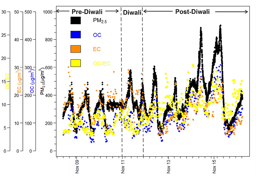
Figure 2. Temporal variability in mass concentrations of PM_2.5 OC, EC, and OC/EC ratio during the study campaign (08th−16th Nov. 2015).

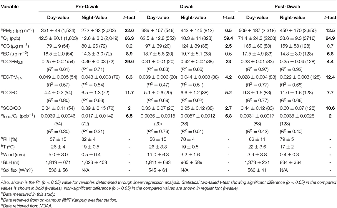
Table 1. Summary statistics of data set [Avg. ± SD (number of samples)] during the sampling period (08th Nov−16th Nov 2015; where 08–10th Nov is considered as Pre-Diwali period, 11th Nov as Diwali, and 12–16th Nov as Post-Diwali period).

The OC/EC ratio varied from 3.2 to 18.5 during the entire study period. The daytime and nighttime average values of OC/EC has been constrained from linear regression analysis (Figure 3). The OC/EC ratio averaged at 4.4 ± 0.2 during the Pre-Diwali daytime period (08th−10th Nov) and was found statistically different as compared to that observed during Pre-Diwali nighttime period (Avg. ± SD = 6.5 ± 1.3; t-value = 11.7, Table 1, Figure 3). Likewise, on Diwali festival event (11th Nov) the daytime (5.1 ± 0.6) and nighttime average values (6.6 ± 1.2) of OC/EC ratio were statistically different (t-value = 5.2). Furthermore, during the Post-Diwali period (12th−16th Nov) the daytime average ratio of OC/EC (9.3 ± 1.5, Figure 3) also looks statistically different as compared to that observed at nighttime (11.0 ± 1.6, t-value = 7.7). Summing up, PM_2.5, OC, and OC/EC ratio were highest during the Post-Diwali period and followed the following trend: Pre-Diwali < Diwali < Post-Diwali. However, EC varied a little during the study period. The higher OC/EC ratio (9–11), during Post-Diwali period plausibly indicated for their predominant emission from biomass burning and/or SOA formation (Rajput et al., 2013, Rajput et al., 2018). To further collect the evidence about this we have carried out concentration weighted trajectory and cluster analysis. We have also retrieved daily fire count imageries for the entire study period from Moderate Resolution Imaging Spectroradiometer sensor (MODIS, onboard NASA Terra and Aqua satellite). We have discussed striking observations revealed from these evidence in subsequent sections.

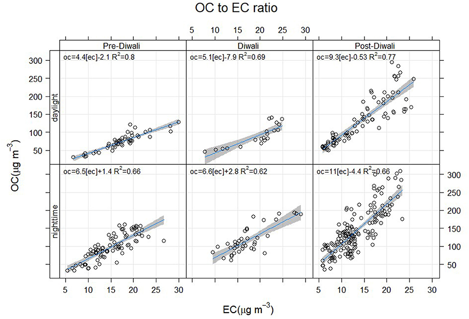
Figure 3. Day and nighttime OC-to-EC ratio based on linear regression analysis (p < 0.05) during Pre-Diwali, Diwali and Post-Diwali periods.

Concentration Weighted Trajectory (CWT) and Cluster Analysis

We have used an open-source GIS-based software viz. TrajStat to carry out the CWT and Cluster Analysis (Figure 4). The application details about CWT and cluster analysis can be found elsewhere (Wang et al., 2009). Briefly, CWT is a receptor-based model and is widely used in conjunction with the cluster analysis to understand the ambient level of air pollutants along with the cluster of trajectories influencing the receptor site (Bansal et al., 2019). Using the CWT and cluster analysis we have attempted to show local/regional source-areas of PM_2.5 potentially affecting the receptor site. To perform CWT and cluster analysis over the study region, a 5-days air-mass back trajectories (AMBTs, GDAS 0.5°m, @ 1,000 m above ground level) data are coupled with PM_2.5 mass concentration data. In the CWT method, each grid cell is assigned a weighted concentration by averaging the sample concentrations based on associated trajectories crossing that grid cell, using the mathematical formula as given below:

where C_ij is the average weighted concentration of PM_2.5 in the grid cell (i, j), M is the total number of trajectories, l is the index of the trajectory, C_l is the concentration observed at receptor site on the arrival of trajectory l, and τ_ijl is the trajectory residence-time (time spent) of trajectory l in the grid cell (i,j). A higher value of C_ij implies that trajectories over the grid cell (i, j) would be associated with higher concentrations. In the cluster analysis method, the measured PM_2.5 mass concentrations were assigned to the corresponding trajectories and the nearest trajectories were clustered according to an angle distance function (Sirois and Bottenheim, 1995).

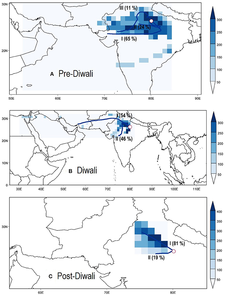
Figure 4. CWT and cluster analysis of PM_2.5 during (A) Pre-Diwali, (B) Diwali, and (C) Post-Diwali study period.

One of the observations from Figure 4 relates that the PM_2.5 levels were relatively high in the north-west (NW) direction of the receptor site (study location, central IGP). Thus, it is expected that if a trajectory cluster is passing more frequently through NW-direction to the receptor site then it will be associated with elevated levels of PM_2.5 (and associated species) as compared to the case when trajectories were arriving from other directions.

Let us now analyze the clusters shown in Figure 4. During Pre-Diwali period (Figure 4A), three sets of clusters have been observed: cluster-I (65%) originated from the west and then traversed through SE to the site, cluster-II (24%) also originated from the west and then traversed through SE to the site but all the time remained closure to the grid-cell of the receptor site, and cluster-III (11%) originated from the west and then traversed through NW to the site. During Diwali (Figure 4B), only two sets of clusters have been observed: cluster-I (54%) showing impact from north-westerly air-masses at the site, whereas cluster-II (46%) originated from the south and then traversed through NW. Thus, based on cluster analysis in conjunction with CWT, relatively high concentrations of PM_2.5 (and associated OC, and OC/EC ratio) during Diwali as compared to those during Pre-Diwali can be explained to more influence of north-westerly polluted air-masses during the Diwali event. During the Post-Diwali period (Figure 4C) also, only two sets of clusters were observed: cluster-I (81%) showing impact from north-westerly air-masses at the site, whereas cluster-II (19%) showed the impact of westerly air masses. Thus, it can be summarized that due to the predominant impact of north-westerly air-masses during the Post-Diwali period the concentrations of PM_2.5, OC (one of the major fractions of PM_2.5) and OC/EC ratio were higher followed by those on Diwali and then on Pre-Diwali period.

To further analyze the plausible reason for showing the elevated levels of air pollutants while air-masses arriving through NW-direction we have retrieved fire count imageries which are discussed below.

Fire Count Imageries Over Indo-Gangetic Plain (IGP)

Moderate Resolution Imaging Spectroradiometer sensor (MODIS, onboard NASA Terra and Aqua satellite) imageries capturing fire count data (spatial resolution: 10 km) from intense open biomass (agricultural-waste paddy-residue) burning over IGP during the study period are shown in Figure 5. Looking at the fire counts data it reveals that agricultural-residue fire activity was relatively intense on 09th, 11th, 12th, 14th, and 16th of Nov, moderate on 10th, 13th, and 15th of Nov, and low on 08th of Nov (Figure 5). Furthermore, it is obvious from the figure that open biomass burning was active in the upwind IGP region (mainly in north-west direction of the sampling site) during the entire study period (08th to 16th November 2015). This observation is quite consistent with earlier observations reporting massive emissions of air pollutants from agricultural-waste burning in upwind IGP (Rajput et al., 2014, 2018). It is worthwhile mentioning that 100s of million tons of paddy-residues are burned every year for the crop-rotation during October–November months in the north-western region of IGP (Rajput et al., 2014). Summing up, clubbing the data set from our campaign, satellite observations on fire counts along with the CWT and cluster analysis it can be summarized that long-range transport of air masses (biomass burning emissions) from NW-direction (upwind IGP) was responsible for elevated levels of air pollutants at the receptor site mainly during Post-Diwali and Diwali period. Before we discuss SOA formation let us look at the research background on the topic.

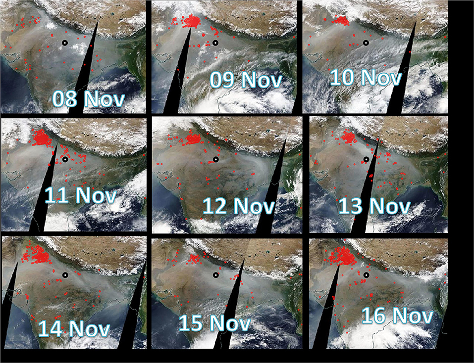
Figure 5. Satellite imageries (Moderate Resolution Imaging Spectroradiometer sensor: MODIS, NASA on board Terra and Aqua satellite) showing fire count data over IGP during study period. The sampling site is shown by black circle.

Research Background on SOA Formation

Chemical transformations of volatile organic compounds (VOCs) can result in the formation of secondary organic aerosols (SOA) and photochemical smog (Volkamer et al., 2006). SOA formation can broadly occur via two pathways: gas- or aqueous-phase oxidation/nitration of VOCs. The oxidation reactions of VOCs can take place with OH radicals, O₃, and H₂O₂ whereas nitration reactions take place with NO₃ radicals. Several studies have compared oxidation/nitration for O₃, OH, and NO₃ radicals. For example, daytime SOA formation through gas-phase oxidation of VOCs (e.g., isoprene, monoterpene) has been reported dominantly by OH radicals and O₃ (Sato et al., 2013; Edwards et al., 2017). However, nighttime dominant SOA formation through gas-phase reactions has been reported by O₃ and NO₃ radical (Sato et al., 2013; Edwards et al., 2017). Furthermore, NO_X and O₃ react with C=C type moieties whereas OH reacts with compounds containing C=C and other saturated though reactive compounds (Palm et al., 2017). Moreover, another oxidizing agent, which oxidizes VOCs efficiently both during the day and nighttime is H₂O₂. A recent study focusing on aqueous-phase SOA led by H₂O₂ during the day (UV aging) and nighttime (dark aging) have brought a new set of information: daytime aqueous-phase oxidation product contains large water clusters [(H₂O)_nOH, n = 14–43], heavier oligomers (m/z: 329–383) whereas nighttime aqueous-phase oxidation products contain small water clusters [(H₂O)_nOH, n = 1–13], small oligomers (m/z: 33–261), and cluster ions (m/z: 333–405) (Zhang et al., 2019). Summing up, the oxidizing agents can led to SOA formation through different pathways. However, the important aspect to mention here is that O₃ has been reported by several aforementioned studies to serve as a potential oxidizing agent both during the day and nighttime.

Let us now discuss regional observations based on several previous studies from Indo-Gangetic Plain (IGP). The IGP experiences high-to-severe air pollution during post-monsoon (Oct–Nov) through winter (Dec–Feb). During the post-monsoon, urban background air pollution in central IGP is regulated mainly by vehicular emission, industrial emission, coal-based power plants, bio-fuel burning, and uplifted mineral dust (Rajput et al., 2016; 2018). Furthermore, long-range transport of pollutants from source-region (in upwind IGP) of seasonally active post-harvest agricultural-waste burning emissions of paddy-residues makes the air quality further poor in central and downwind locations (Rajput et al., 2014). There have been several attempts on measurements and modeling of various air pollutants, secondary organic aerosol (SOA) formation, and radiative forcing estimates across IGP, e.g., (Ram et al., 2008; Srivastava and Ramachandran, 2013; Rajput et al., 2018; Dumka et al., 2019; Srivastava et al., 2019; Mhawish et al., 2020; Mishra and Kulshrestha, 2020; Satish et al., 2020). Association between pollutants has been reported from the above studies in particular and other studies conducted across the globe in general. However, the causation of an exposure variable on an outcome in atmospheric and aerosol chemistry space has never been studied before (to the best of our knowledge).

Diurnal Variability of f_SOC, f_POC, O₃, BLH, RH, and T

The diurnal variability of the fraction of SOC and POC in total OC represented as f_SOC and f_POC, respectively are shown in Figures 6A–C for Pre-Diwali, Diwali, and Post-Diwali periods. Accordingly, during Pre-Diwali period the average f_SOC was relatively high during nighttime (0.39 ± 0.15, t-value = 2.0) as compared to that in daytime (0.34 ± 0.11, Figure 6A). During Diwali, daytime average value of f_SOC (0.33 ± 0.07) was higher than that in nighttime (0.25 ± 0.12, t-value = 2.7). Similarly, during Post-Diwali, daytime average value of f_SOC (0.44 ± 0.12) was also higher than that in nighttime (0.30 ± 0.07, t-value = 10.6). Thus, unlike the Pre-Diwali period, the average f_SOC was higher in the daytime as compared to that in nighttime during Diwali and Post-Diwali periods (Figures 6B,C). We reiterate that the impact of long-range transport of pollutants from post-harvest biomass burning emissions were observed during Diwali and Post-Diwali period. Thus, it is logical to infer that under the impact of biomass burning emissions, the f_SOC value was observed higher in the daytime as compared to that in the nighttime. The pattern of f_POC is also shown in Figure 6 but since it is trivial to estimate f_POC (= 1–f_SOC) we do not discuss here about it in the detail.

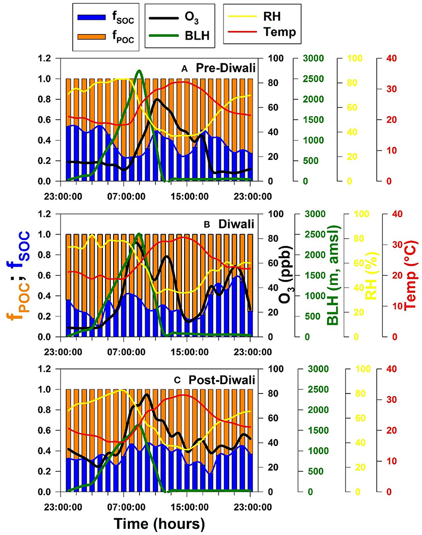
Figure 6. Temporal variability of f_SOC, f_POC, O₃ (ppb), BLH (m), RH (%) and temperature (°C) during (A) Pre-Diwali, (B) Diwali, and (C) Post-Diwali period.

We have also shown the diurnal variability of O₃, BLH, RH, and temperature (T) during the study period (Figure 6). The O₃ has a daytime peak during Pre-Diwali whereas during Diwali and Post-Diwali periods it exhibited an additional peak in the nighttime. The nighttime O₃ peak is attributable to the long-range transport of biomass burning emissions from NW-direction (upwind IGP). Furthermore, RH and T retained their variability pattern during the entire study period. Moreover, maximum BLH during Pre-Diwali (~2,700 m, asl.), and Diwali (2,500 m asl.) were relatively high as compared to maximum BLH recorded during Post-Diwali (1,500 m, asl.). However, the diurnal variability pattern of BLH looks similar during the entire study period. Before we move to the next aspect, there are two important observations to notice for (from Figure 6): BLH variability appears to have an insignificant impact on f_SOC pattern, and BLH explains, if not all, at least some of the variability of O₃. This is exactly the scenario we were referring to in the above section wherein we discussed the validity of BLH to serve as IV to infer the causal effect of O₃ (exposure) on f_SOC (outcome). Before we discuss the results from IVA analysis (all relevant equations given above), let us first look at the collinearity between f_SOC and O₃ using linear regression analysis.

Correlation Analyses: O₃ vs. f_SOC (= SOC/OC Ratio)

A 3-D correlation plot is shown in Figure 7 for three events (Pre-Diwali, Diwali, and Post-Diwali) and two periods (daylight and nighttime). O₃ (ppb) is plotted on the X-axis, f_SOC on the Y-axis, and the BLH data set is plotted on the z-axis (m, shown on a scale at the right hand side of the plot). The BLH appears to have an insignificant influence on the relationship between f_SOC and O₃. This further relates to our aforementioned observation on insignificant co-variability of f_SOC as a function of BLH. For the linear regression analysis as shown in Figure 7, the level of significance was found to be quite satisfactory (i.e., p < 0.05) only for two cases: daytime of Diwali and Post-Diwali period. During Diwali daytime period, the ratio of f_SOC/O₃ (ppb⁻¹) averaged at 0.0036 ± 0.0015 (R² = 0.79, p < 0.05, Table 1, Figure 7). Furthermore, during the Post-Diwali period, the average ratio of f_SOC/O₃ (ppb⁻¹) was 0.0031 ± 0.0017 (R² = 0.42, p < 0.05, Table 1, Figure 7). Thus, during the daytime period marked with long-range transport of pollutants from biomass burning emission the association between f_SOC and O₃ was found to be quite significant in this study. However, based on linear regression analysis, we cannot attribute that how much SOA (f_SOC) has been formed due to the O₃ during daytime of Diwali and Post-Diwali period? So, the next step would be to apply causal modeling to gain further insights on this aspect.

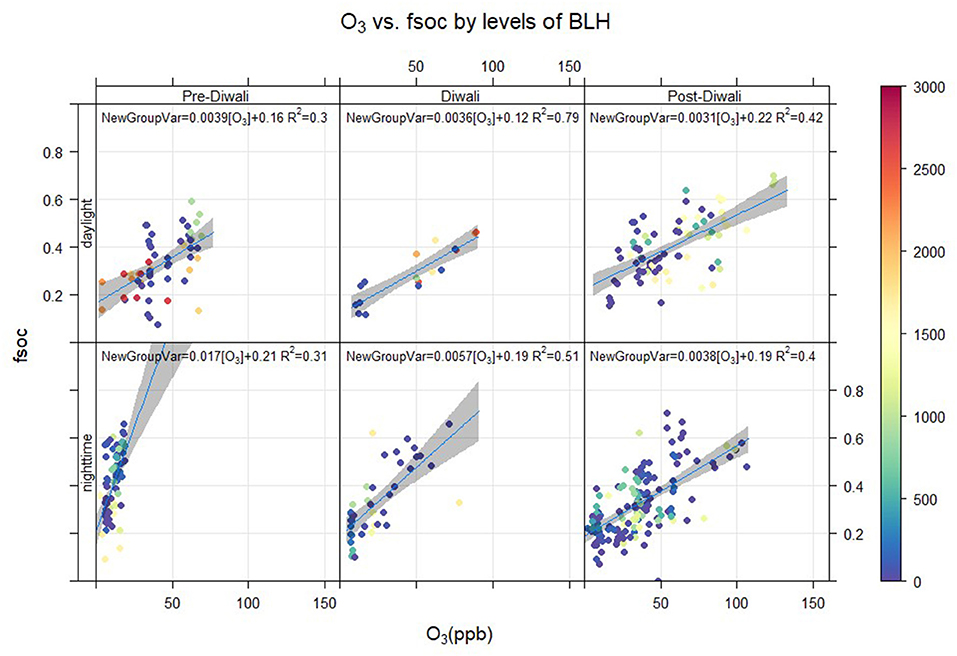
Figure 7. Linear regression analysis of f_soc (= SOC/OC) against O₃ (ppb) by levels of BLH (m) in day and nighttime during Pre-Diwali, Diwali and Post-Diwali periods.

The Causal Effect of O₃ on SOA Formation

We have performed IVA analysis to assess the causal effect of O₃ on SOA formation in IGP. We have used a support vector machine (SVM, R package e1071) (Cortes and Vapnik, 1995; Team, 2013) with a radial kernel to estimate variation in O₃ (exposure) explained by the BLH (instrument). The SVM algorithm maximizes a 10-fold cross-validation. We have checked R² of the instrument (BLH) predicting exposure (O₃) to ensure that our instrument was strongly associated with the exposure. In this process of validation, for all the six cases (daytime and nighttime of Pre-Diwali, Diwali, and Post-Diwali) the R² varied between 0.84 and 0.93, thus suggesting BLH to serve as a good instrument to estimate the causal effect of O₃ on SOA formation. We have already discussed above in detail about the mathematical modeling of IVA to infer causal effect of O₃ on SOA formation (i.e., f_SOC). The results of the IVA analysis are shown in Table 2. Before we discuss the results, let us recall that only if the Null hypothesis is rejected (i.e., β₁ ≠ 0), we can get a causal estimate of O₃ on SOA formation. Now, if we look at the 95% confidence interval values (CI, Table 2) then it can be noticed that only for the two cases i.e., daytime of Diwali and Post-Diwali period, the null hypothesis is rejected (i.e., β₁ ≠ 0). Thus, causal estimate can be obtained for the aforementioned two cases only during the study period.

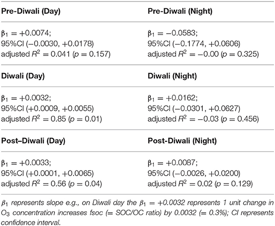
Table 2. Summary of instrumental variable analysis (IVA) estimating causal effect of O₃ on f_SOC.

The IVA analysis revealed that during Diwali daytime period, the average ratio of f_SOC/O₃ (ppb⁻¹) was 0.0032 (95% CI: 0.0009, 0.0055, p < 0.05, Table 2). Furthermore, during the Post-Diwali daytime period, the average ratio of f_SOC/O₃ (ppb⁻¹) was 0.0033 (95% CI: 0.0001, 0.0065, p < 0.05, Table 2). Thus, based on IVA it is inferred that O₃ has a causal effect on SOA formation during daytime while experiencing massive emissions from long-range transport of biomass burning emissions at the receptor site.

Conclusions

This study finds and discusses the application of instrumental variable analysis (IVA) for inferring causality in atmospheric and aerosol chemistry observations. The basic methodology of IVA has been explained herein through a set of equations and theories involved concisely. IVA is a quasi-experimental design that can control for measured as well as unmeasured confounders. BLH and wind speed have been suggested to serve as good instruments for inferring causality in atmospheric chemical transformations. The importance of randomized experiments to achieve exchangeability has been explained in terms of obtaining the same distribution of confounders in measured and unmeasured data points. The machine learning algorithm has been used to assess the validity of the instrument. On field-based measurements, the IVA has been applied to get a causal estimate of the outcome (e.g., SOA formation) due to the exposure (O₃). Accordingly, the average ratio of f_SOC/O₃ (ppb⁻¹) was found to be 0.0032 (95% CI: 0.0009, 0.0055) and 0.0033 (95% CI: 0.0001, 0.0065) during daytime of Diwali and Post-Diwali period. However, during rest of the study period the relationship between O₃ and f_SOC was not significant. Inferences from IVA coupled with the CWT, cluster analysis, and fire count imageries revealed that O₃ has a causal effect on SOA formation during the daytime when emissions from biomass burning via long-range transport influenced the receptor site. The programming of IVA can be done using R, python, or any other language-based software.

Data Availability Statement

The original contributions presented in the study are included in the article/Supplementary Materials, further inquiries can be directed to the corresponding author/s.

Author Contributions

IVA has been performed by PR. The manuscript has been conceptualized and written by PR. The field-campaign was planned and organized by PR and TG. All authors contributed to the article and approved the submitted version.

Conflict of Interest

The authors declare that the research was conducted in the absence of any commercial or financial relationships that could be construed as a potential conflict of interest.

Acknowledgments

PR was thankful to Prof. Joel Schwartz (Harvard School of Public Health, Boston) for introducing the causal modeling. We thank the reviewers for providing constructive comments and suggestions.

Supplementary Material

The Supplementary Material for this article can be found online at: https://www.frontiersin.org/articles/10.3389/fenvs.2020.566136/full#supplementary-material

References

Bansal, O., Singh, A., and Singh, D. (2019). Characteristics of Black carbon aerosols over Patiala Northwestern part of the IGP: source apportionment using cluster and CWT analysis. Atmos. Poll. Res. 10, 244–256. doi: 10.1016/j.apr.2018.08.001
Birch, M. E., and Cary, R. A. (1996). Elemental carbon-based method for monitoring occupational exposures to particulate diesel exhaust. Aerosol. Sci. Technol. 25, 221–241. doi: 10.1080/02786829608965393
Carslaw, D. C., and Ropkins, K. (2012). openair — An R package for air quality data analysis. Environ. Modell. Softw. 27–28, 52–61. doi: 10.1016/j.envsoft.2011.09.008
Castro, L. M., Pio, C. A., Harrison, R. M., and Smith, D. J. T. (1999). Carbonaceous aerosol in urban and rural European atmospheres: estimation of secondary organic carbon concentrations. Atmos. Environ. 33, 2771–2781. doi: 10.1016/S1352-2310(98)00331-8
Cortes, C., and Vapnik, V. (1995). Support-vector networks. Mach. Learn. 20, 273–297. doi: 10.1007/BF00994018
Dong, J., Crow, W. T., Duan, Z., Wei, L., and Lu, Y. (2019). A double instrumental variable method for geophysical product error estimation. Remote Sens. Environ. 225, 217–228. doi: 10.1016/j.rse.2019.03.003
Draxler, R. R., and Rolph, G. D. (2003). HYSPLIT (Hybrid Single-Particle Lagrangian Integrated Trajectory) Model access via NOAA ARL READY Website. Avialble online at: http://www.arl.noaa.gov/ready/hysplit4.html. Silver Spring, MD: NOAA Air Resources Laboratory
Dumka, U. C., Tiwari, S., Kaskaoutis, D. G., Soni, V. K., Safai, P. D., and Attri, S. V. (2019). Aerosol and pollutant characteristics in Delhi during a winter research campaign. Environ. Sci. Pollut. Res. 26, 3771–3794. doi: 10.1007/s11356-018-3885-y
Edwards, P., Aikin, K. C., Dube, W. P., Fry, J. L., Gilman, J. B., de Gouw, J. A., et al. (2017). Transition from high- to low-NOx control of night-time oxidation in the southeastern US. Nat. Geosci. 10, 490–495. doi: 10.1038/ngeo2976
Izhar, S., Rajput, P., and Gupta, T. (2018). Variation of particle number and mass concentration and associated mass deposition during diwali festival. Urban Clim. 24, 1027–1036. doi: 10.1016/j.uclim.2017.12.005
Lind, J. T. (2020). Rainy day politics. An instrumental variables approach to the effect of parties on political outcomes. Eur. J. Political Econ. 61:101821. doi: 10.1016/j.ejpoleco.2019.101821
Mhawish, A., Banerjee, T., Sorek-Hamer, M., Bilal, M., Lyapustin, A. I., Chatfield, R., et al. (2020). Estimation of high-resolution pm2.5 over the indo-gangetic plain by fusion of satellite data, meteorology, and land use variables. Environ. Sci. Technol. 54, 7891–7900. doi: 10.1021/acs.est.0c01769
Mishra, M., and Kulshrestha, U. (2020). Extreme air pollution events spiking ionic levels at urban and rural sites of indo-gangetic plain. Aerosol Air Qual. Res. 20, 1266–1281. doi: 10.4209/aaqr.2019.12.0622
Palm, B. B., Campuzano-Jost, P., Day, D. A., Ortega, A. M., Fry, J. L., Brown, S. S., et al. (2017). Secondary organic aerosol formation from in situ OH, O3, and NO3 oxidation of ambient forest air in an oxidation flow reactor. Atmos. Chem. Phys. 17, 5331–5354. doi: 10.5194/acp-17-5331-2017
Pitz, M., Cyrys, J., Karg, E., Wiedensohler, A., Wichmann, H. E., and Heinrich, J. (2003). Variability of apparent particle density of an urban aerosol. Environ. Sci. Technol. 37, 4336–4342. doi: 10.1021/es034322p
Rajput, P., Anjum, M. H., and Gupta, T. (2017). One year record of bioaerosols and particles concentration in Indo-Gangetic Plain: implications of biomass burning emissions to high-level of endotoxin exposure. Environ. Pollut. 224, 98–106. doi: 10.1016/j.envpol.2017.01.045
Rajput, P., Izhar, S., and Gupta, T. (2019). Deposition modeling of ambient aerosols in human respiratory system: health implication of fine particles penetration into pulmonary region, Atmos. Poll. Res, 10, 334–343. doi: 10.1016/j.apr.2018.08.013
Rajput, P., Mandaria, A., Kachawa, L., Singh, D. K., Singh, A. K., and Gupta, T. (2016). Chemical characterization and source-apportionment of PM1 during massive loading at an urban location in Indo-Gangetic plain: impact of local sources and long-range transport. Tellus B Chem. Phys. Meteorol. 68:30659. doi: 10.3402/tellusb.v68.30659
Rajput, P., Sarin, M. M., and Kundu, S. S. (2013). Atmospheric particulate matter (PM2.5), EC, OC, WSOC and PAHs from NE-Himalaya: Abundances and chemical characteristics. Atmos. Poll. Res. 4, 214–221. doi: 10.5094/APR.2013.022
Rajput, P., Sarin, M. M., Sharma, D., and Singh, D. (2014). Characteristics and emission budget of carbonaceous species from post-harvest agricultural-waste burning in source region of the Indo-Gangetic plain. Tellus B Chem. Phys. Meteorol. 66:21026. doi: 10.3402/tellusb.v66.21026
Rajput, P., Singh, D. K., Singh, A. K., and Gupta, T. (2018). Chemical composition and source-apportionment of sub-micron particles during wintertime over northern india: New insights on influence of fog-processing. Environ. Poll. 233, 81–91. doi: 10.1016/j.envpol.2017.10.036
Ram, K., Sarin, M. M., and Hegde, P. (2008). Atmospheric abundances of primary and secondary carbonaceous species at two high-altitude sites in India: sources and temporal variability. Atmos. Environ. 42, 6785–6796. doi: 10.1016/j.atmosenv.2008.05.031
Satish, R., Rastogi, N., Singh, A., and Singh, D. (2020). Change in characteristics of water-soluble and water-insoluble brown carbon aerosols during a large-scale biomass burning. Environ. Sci. Pollut. Res. 27, 33339–33350. doi: 10.1007/s11356-020-09388-7
Sato, K., Inomata, S., Xing, J. H., Imamura, T., Uchida, R., Fukuda, S., et al. (2013). Effect of OH radical scavengers on secondary organic aerosol formation from reactions of isoprene with ozone, Atmos. Environ. 79, 147–154. doi: 10.1016/j.atmosenv.2013.06.036
Schwartz, J., Bind, M. A., and Koutrakis, P. (2017). Estimating causal effects of local air pollution on daily deaths: effect of low levels. Environ. Health Perspect. 125, 23–29. doi: 10.1289/EHP232
Schwartz, J., Fong, K., and Zanobetti, A. (2018). A national multicity analysis of the causal effect of local pollution, NO2, and PM2.5 on mortality, Environ. Health Perspect. 126:087004. doi: 10.1289/EHP2732
Sirois, A., and Bottenheim, J. W. (1995). Use of backward trajectories to interpret the 5-year record of PAN and O3 ambient air concentrations at Kejimkujik National Park, Nova Scotia. J. Geophys. Res. 100, 2867– 2881. doi: 10.1029/94JD02951
Srivastava, P., Dey, S., Srivastava, A. K., Singh, S., and Tiwari, S. (2019). Suppression of aerosol-induced atmospheric warming by clouds in the Indo-Gangetic Basin, northern India. Theor. Appl. Climatol. 137, 2731–2741. doi: 10.1007/s00704-019-02768-1
Srivastava, R., and Ramachandran, S. (2013). The mixing state of aerosols over the Indo-Gangetic Plain and its impact on radiative forcing. Q. J. R. Meteorol. Soc. 139, 137–151. doi: 10.1002/qj.1958
Stein, A. F., Draxler, R. R., Rolph, G. D., Stunder, B. J. B., Cohen, M. D., and Ngan, F. (2015). NOAA's HYSPLIT atmospheric transport and dispersion modeling system. Bull. Am. Meteorol. Soc. 96, 2059–2077. doi: 10.1175/BAMS-D-14-00110.1
Team, R. C. (2013). R: A Language and Environment for Statistical Computing. Vienna: R Foundation for Statistical Computing.
Volkamer, R., Jimenez, J. L., Martini, F. S., Dzepina, K., Zhang, Q., Salcedo, D., et al. (2006). Secondary organic aerosol formation from anthropogenic air pollution: rapid and higher than expected. Geophys. Res. Lett. 33:L17811. doi: 10.1029/2006GL026899
von Hinke, S., Smith, G. D., Lawlor, D. A., Propper, C., and Windmeijer, F. (2016). Genetic markers as instrumental variables. J. Health Econ. 45, 131–148. doi: 10.1016/j.jhealeco.2015.10.007
Wang, Y. Q., Zhang, X. Y., and Draxler, R. R. (2009). TrajStat: GIS-based software that uses various trajectory statistical analysis methods to identify potential sources from long-term air pollution measurement data. Environ. Modell. Softw. 24, 938–939. doi: 10.1016/j.envsoft.2009.01.004
Young-Xu, Y., Snider, J. T., van Aalst, R., Mahmud, S. M., Thommes, E. W., Lee, J. K. H., et al. (2019). Analysis of relative effectiveness of high-dose versus standard-dose influenza vaccines using an instrumental variable method, Vaccine 37, 1484–1490. doi: 10.1016/j.vaccine.2019.01.063
Keywords: causal inference, machine learning, air pollution, atmospheric chemistry, aerosols
Citation: Rajput P and Gupta T (2020) Instrumental Variable Analysis in Atmospheric and Aerosol Chemistry. Front. Environ. Sci. 8:566136. doi: 10.3389/fenvs.2020.566136
Received: 27 May 2020; Accepted: 30 November 2020;
Published: 21 December 2020.
Edited by:
Nina Jasmin Schleicher, Imperial College London, United KingdomReviewed by:
Jai Prakash, Washington University in St. Louis, United StatesDominik Weiss, Imperial College, Pakistan
Copyright © 2020 Rajput and Gupta. This is an open-access article distributed under the terms of the Creative Commons Attribution License (CC BY). The use, distribution or reproduction in other forums is permitted, provided the original author(s) and the copyright owner(s) are credited and that the original publication in this journal is cited, in accordance with accepted academic practice. No use, distribution or reproduction is permitted which does not comply with these terms.
*Correspondence: Prashant Rajput, prashant.rajput@phfi.org; prajput.prl@gmail.com