


1 Introduction
An area of interest in linguistics is how much of human language is innate and how much is learned from data (e.g. Chomsky Reference Chomsky1988, Elman et al. Reference Elman, Bates, Johnson, Karmiloff-Smith, Parisi and Plunkett1996, Pullum & Scholz Reference Pullum and Scholz2002, Tomasello Reference Tomasello2003). From this perspective, the question of how much information about phonological categories can be retrieved strictly from distributional information is of considerable importance to the field of phonology.
One of the central observations of phonological theory is that speech sounds tend to pattern according to phonetic similarity, both within and across languages (Chomsky & Halle Reference Chomsky and Halle1968, Mielke Reference Mielke2008). For example, processes like final obstruent devoicing, where voiced obstruents become voiceless word- or syllable-finally, are common across languages (Wetzels & Mascaró Reference Wetzels and Mascaró2001). Despite the differences in place and manner of articulation across these sounds, two shared phonetic properties allow them to be treated as a single class: substantial impedance of airflow out of the vocal tract, and vocal fold vibration.
Based on this robust typological generalisation, classic work has suggested that there is a universal tendency for language learners to group sounds based on their phonetic properties (e.g. Chomsky & Halle Reference Chomsky and Halle1968). Languages may use classes differently in their phonologies, but in principle the set of classes available across languages should be the same, by virtue of shared human physiology.
There is evidence, however, for the existence of classes that do not appear to be phonetically coherent, such as the Sanskrit ‘ruki’ class (Vennemann Reference Vennemann1974), the triggers for Philadelphia /æ/-tensing (Labov et al. Reference Labov, Ash and Boberg2006) and Cochabamba Quechua, where etymological /q/ has become [ʁ], but still patterns with the voiceless stops (Gallagher Reference Gallagher2019). Mielke (Reference Mielke2008) presents many such cases. Instances of variable patterning of a segment across languages also bear on this issue. For example, /l/ varies in whether it is treated as [+continuant] or [―continuant] in languages (Mielke Reference Mielke2008).
These observations have led some researchers to propose that phonological classes may be learned and language-specific (Mielke Reference Mielke2008, Dresher Reference Dresher2014, Archangeli & Pulleyblank Reference Archangeli, Pulleyblank, Hannahs and Bosch2018, among others). Under such theories, phonologically salient classes need not be phonetically coherent, and distributional learning must account for a larger part of phonological acquisition than previously thought. That is, a phonological class is identified based (at least in part) on how its members pattern in the language, rather than some shared phonetic quality.
The typological observation that classes tend to be phonetically coherent is accounted for by suggesting a tendency for similar sounds to undergo similar phonetically driven diachronic processes (Blevins Reference Blevins2004). In other words, typology is governed primarily by pressures on language transmission, rather than biases on the part of the learner. These pressures will tend to generate phonetically natural outcomes, though unnatural outcomes can also occur (Beguš Reference Beguš2018a, Reference Begušb). This claim remains controversial (Kiparsky Reference Kiparsky2006), though unnatural outcomes have been frequently documented (e.g. Bach & Harms Reference Bach, Harms, Stockwell and Macaulay1972, Mielke Reference Mielke2008, Scheer Reference Scheer, Honeybone and Salmons2015).
Regardless of whether one is willing to commit to the position of emergent classes, these ideas raise theoretically interesting questions. Namely, to what extent are phonological classes apparent in the distribution of sounds in a language, and to what extent do learners make use of this information?
For a class to be apparent in the distribution of sounds in a language, the sounds in that class must impose similar restrictions on which sounds may occur nearby, and this effect must be learnable, i.e. robust enough to be detectable by some learning algorithm. Distribution is, however, only one source of information available to the human learner. Even if a class is apparent in the input data, this does not mean that learners are bound to use it. It may be the case that learners rely on such information only when it is robust enough to override other (possibly conflicting) influences, such as phonetic information or learning biases (see e.g. Moreton Reference Moreton2008, Hayes et al. Reference Hayes, Zuraw, Siptár and Londe2009).
This paper investigates the learning of phonological classes when only distributional information is available. That is, it deals with the question of what classes are apparent, rather than what the learner might actually use. It does so by constructing an algorithm that attempts to learn solely from the contexts in which sounds occur, building on past work (e.g. Goldsmith & Xanthos Reference Goldsmith and Xanthos2009, Nazarov Reference Nazarov2014, Reference Nazarov2016). Again, this is not to suggest that phonetic information is not important for characterising phonological classes: rather, it is an attempt to see how far we can get while restricting ourselves to only one of the many available sources of information.
The algorithm consists of the four components in (1), each of which contributes to accurate learning of phonological classes.
-
(1)


Steps (c) and (d) are recursively performed on the discovered classes, allowing classes of different sizes to be found (§5.4).
Aside from eschewing phonetic information, this algorithm operates with two additional assumptions. First, it uses only phonotactic information: there is no explicit attempt to capture alternations. Although this may be a reasonable assumption about the initial phonological learning done by infants (e.g. Hayes Reference Hayes2004, Prince & Tesar Reference Prince and Tesar2004, Jarosz Reference Jarosz2006), it is adopted here merely as a simplifying assumption. Second, the algorithm assumes that the learner has access to a segmental representation of speech (e.g. Lin Reference Lin2005, Feldman et al. Reference Feldman, Griffiths, Goldwater and Morgan2013).
The algorithm produces a set of phonological classes that may be viewed as implicitly reflecting a feature system, in that any class contained in this set can be uniquely characterised by some combination of feature/value pairs. The process of deriving an explicit feature system from a set of classes is described in a related paper (Mayer & Daland Reference Mayer and Daland2019).
This paper is structured as follows. §2 reviews past research that has taken a distributional approach to learning phonological structure. §3 describes a toy language with well-defined phonotactic properties, which serves as a running example and a basic test case for the algorithm. The next two sections describe the components of the algorithm. §4 details how a normalised vector representation of the sounds of a language can be generated from a phonological corpus. §5 shows how a combination of Principal Component Analysis and clustering algorithms can be used to extract phonological classes from such embeddings, and details its performance on the toy language. §6 applies the algorithm to Samoan, English, French and Finnish. It is able to successfully distinguish consonants and vowels in every case, and retrieves interpretable classes within those categories for each language. §7 compares these results against past work, and §8 offers discussion and proposals for future research.
2 Previous work
Distributional learning has been proposed in most areas of linguistics, suggesting that it may be a domain-general process. Examples include word segmentation and morphology (e.g. Saffran et al. Reference Saffran, Newport and Aslin1996, Goldsmith Reference Goldsmith, Clark, Fox and Lappin2010), syntax (e.g. Harris Reference Harris1946, Redington et al. Reference Redington, Crater and Finch1998, Wonnacott et al. Reference Wonnacott, Newport and Tanenhaus2008) and semantics (e.g. Andrews et al. Reference Andrews, Vigliocco and Vinson2009).
Distributional approaches to phonology were explored by a number of pre-generative phonologists, but this work was limited by technological factors, and is not well-known today (see Goldsmith & Xanthos Reference Goldsmith and Xanthos2008: App. A). More powerful computers, together with advances in statistical and machine learning research, have recently rendered such approaches more viable.Footnote 1
Powers (Reference Powers1997) provides a detailed comparison of early work building on these advances. Notable additions include vector representations of sounds, normalisation to probabilities and the use of matrix factorisation and bottom-up clustering algorithms to group sounds together. While these approaches are a notable step forward, they frequently fail to distinguish between consonants and vowels in English. This should be taken with some caution, however, as Powers ran his evaluations on orthographic data, whose vowels (a, e, i, o, u and sometimes y) do not map straightforwardly onto phonemic vowels.
In the same period, Ellison (Reference Ellison1991, Reference Ellison1992) explored a minimum description length analysis, which uses an information-theoretic objective function to evaluate how well a set of classes fits an observed dataset. Ellison reports that his method is generally successful in differentiating consonants and vowels across a wide range of languages, as well as identifying aspects of harmony systems. He also runs his models on orthographic data.
In more recent work, Goldsmith & Xanthos (Reference Goldsmith and Xanthos2009) compare three approaches to learning phonological classes in English, French and Finnish. The first, Sukhotin's algorithm, is mostly of historical interest, but can differentiate between consonants and vowels reasonably well, using calculations simple enough to be performed by hand. The second uses spectral clustering, which models distributional similarity between segments as an undirected graph with weighted edges. By finding an optimal partition of the graph into two or more groups, Goldsmith & Xanthos are able to successfully distinguish between consonants and vowels, and provide a basic characterisation of harmony systems. The third uses maximum likelihood Hidden Markov Models. Maximum likelihood estimation is used to learn transition and emission probabilities for a finite-state machine with a small number of states (e.g. two for vowel vs. consonant). The ratio of emission probabilities for each segment between states can then be used to classify them. This approach works well for distinguishing vowels and consonants, identifying vowel harmony, and (to some extent) syllable structure.
Calderone (Reference Calderone2009) uses a similar approach to spectral clustering, independent component analysis, which decomposes a matrix of observed data into a mixture of statistically independent, non-Gaussian components. This results in a qualitative separation between consonants and vowels, as well as suggesting finer-grained distinctions within these sets.
Taking a different approach, Nazarov (Reference Nazarov2014, Reference Nazarov2016) details an algorithm for jointly learning phonological classes and constraints using a combination of maximum entropy Optimality Theory and Gaussian mixture models. Nazarov's method calculates the information gain from introducing a constraint that penalises a segment in a particular context, then clusters segments based on this information gain, using a Gaussian mixture model. Segments that are clustered together are hypothesised to form a class, and specific constraints are in turn combined into more general ones using these classes. This performs well on a simple artificial language.
Finally, recent work has used neural networks to learn phonological structure from distribution. Silfverberg et al. (Reference Silfverberg, Mao and Hulden2018) use a recurrent neural network to generate phoneme embeddings. They show that these embeddings correlate well with embeddings based on phonological features, but do not attempt to explicitly identify classes. Their non-neural comparison model employs vector embedding, singular value decomposition, and normalisation using positive pointwise mutual information, all of which are used in the algorithm presented in this paper, but it does not take phoneme ordering into account. Similarly, Mirea & Bicknell (Reference Mirea and Bicknell2019) generate phoneme embeddings using a long-term short-term memory neural network, and perform hierarchical clustering on these embeddings. This clustering does not cleanly separate consonants and vowels, though some suggestive groupings are present.
The goal of this paper is to expand on the successes of this ongoing collective research programme. The algorithm described below shares many aspects with past work, such as vector embedding (Powers Reference Powers1997, Calderone Reference Calderone2009, Goldsmith & Xanthos Reference Goldsmith and Xanthos2009, Nazarov Reference Nazarov2014, Reference Nazarov2016, Silfverberg et al. Reference Silfverberg, Mao and Hulden2018, Mirea & Bicknell Reference Mirea and Bicknell2019), normalisation (Powers Reference Powers1997, Silfverberg et al. Reference Silfverberg, Mao and Hulden2018), matrix decomposition (Powers Reference Powers1997, Calderone Reference Calderone2009, Goldsmith & Xanthos Reference Goldsmith and Xanthos2009, Silfverberg et al. Reference Silfverberg, Mao and Hulden2018) and clustering algorithms (Powers Reference Powers1997, Nazarov Reference Nazarov2014, Reference Nazarov2016, Mirea & Bicknell Reference Mirea and Bicknell2019). The innovations that will be presented below are largely in the combination and extension of these techniques, but the clustering methodology presented is relatively novel.
These innovations allow for the retrieval of classes that stand in a complex relationship to one another in an artificial language. They also enable the learning of finer-grained categories in natural languages, while requiring fewer assumptions than past work. The modular structure of the algorithm also provides a useful general framework in which further studies of distributional learning might proceed. The current implementation of this algorithm is available in the online supplementary materials, and researchers are encouraged to use and modify it freely.Footnote 2
3 Parupa: an artificial language
Because it is not clear a priori what classes might be apparent in the distribution of a natural language, it is useful to begin with a case where the target classes are known in advance, a practice adopted in past work (Goldsmith & Xanthos Reference Goldsmith and Xanthos2009, Nazarov Reference Nazarov2014, Reference Nazarov2016). To this end, I introduce an artificial language called Parupa, which has well-defined phonotactic properties.Footnote 3 Parupa serves as a running example throughout the paper and as an initial test case for the algorithm. Its consonant and vowel inventories are shown in (2).
-
(2)

Parupa has the distributional properties in (3).
-
(3)

Note that although these properties vary in their ‘phonetic naturalness’, there is no notion of phonetic substance in this model. These particular properties were chosen in part to emphasise that the distributional learning algorithm does not distinguish between natural and unnatural patterns. More importantly, they were chosen to produce multiple, overlapping partitions of the sets of vowels and consonants. For example, the vowel set is partitioned in two different ways: high–mid and front–back. This structure is common in natural languages, and introduces challenges for many clustering algorithms (§5). Given these properties, the algorithm should retrieve at least the classes shown in Fig. 1.
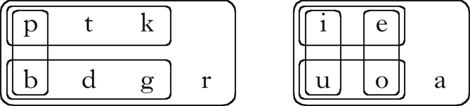
Figure 1 The phonological classes of Parupa.
A language corpus was generated using a Hidden Markov Model (see Appendix A).Footnote 4 Although each segment was equally likely to occur in environments where it is phonologically licit, the phonotactic constraints meant that not all segments were equally common in the corpus (for example, /a/ was the most frequent vowel). The generated corpus had 50,000 word tokens, resulting in about 18,000 word types. The input to the algorithm consists only of the word types.Footnote 5 Examples of Parupa words are given in (4).
-
(4)

4 Quantifying similarity: vector space models
This model operates under the assumption that elements in the same category should have similar distributions (e.g. Harris Reference Harris1946, Mielke Reference Mielke2008). A distribution is a description of how frequently each of a set of possible outcomes is observed. Here the elements we are interested in are sounds, the categories are phonological classes, and the outcomes are the contexts in which a sound occurs, i.e. the other sounds that occur near it.
This assumption can be broken down into two parts. The first is that if two sounds participate in the same phonological pattern, they must share some abstract representational label: the label indicates the ‘sameness’ of the two sounds with respect to this pattern. In this case, the labels we are interested in are featural specifications reflecting class membership. The second is that all abstract representational labels must be discoverable from some phonological pattern, hence for every abstract representational label there will be a phonological pattern that uses this label. That is, we should not expect the learner to posit abstract structure in the absence of some detectable influence on the data. This is similar to assumptions made in work on hidden structure learning (e.g. Tesar & Smolensky Reference Tesar and Smolensky2000), though it is stronger in suggesting that the existence of a label, and not only its assignment to overt forms, is conditioned by phonological patterns.
To quantify the distributions of each sound, I adopt vector space modelling. The principle behind this approach is to represent objects as vectors or points in an n-dimensional space whose dimensions capture some of their properties. Embedding objects in a vector space allows for convenient numerical manipulation and comparison between them.
This approach is commonly applied in many language-related domains (Jurafsky & Martin Reference Jurafsky and Martin2008): in document retrieval, where documents are represented by vectors whose dimensions reflect words that occur in the document, in computational semantics, where words are represented by vectors whose dimensions reflect other words that occur near the target word, and in speech/speaker recognition, where sounds are represented by vectors whose components are certain acoustic parameters of the sound. This is also essentially the approach taken in many of the papers discussed above, where sounds are represented as vectors whose dimensions reflect counts of sounds that occur near them. Whether we are dealing with documents, words or sounds, the projection of these objects into a vector space should be done in such a way that similar objects end up closer in the space than less similar ones. An important distinction between applying this approach to documents or words and applying it to sounds is that order is crucially important for sounds. In the applications above, it is generally more useful to know that a word occurs in a document or that a word occurs near another word than it is to know that a word is the nth word in a document, or that a word occurs exactly n words before another word. In contrast, ordering is crucial for phonology, since adjacency and directionality play important roles in phonological processes.Footnote 6 I generate embeddings by combining aspects of the approaches described above. Before going into more detail, I will provide a simple, concrete example of how we can construct a vector representation of sounds in a phonological corpus.
4.1 A simple vector embedding of sounds
Suppose we have a language with only two sounds, /t/ and /a/, and a corpus containing the five words in (5).
-
(5)
Σ is the set of all unique symbols in the corpus. There is an additional symbol not in Σ, #, which represents a word boundary.Footnote 7 Here Σ = {t, a}.
To go from this corpus to a vector representation of the sounds, we must decide how to define the dimensions of the vector space, i.e. which aspects of a sound's distribution we wish the model to be sensitive to, and how these aspects should be quantified. For this simple example, I will define each dimension as the bigram count of the number of times a particular symbol occurs immediately before the target symbol. The corresponding vector for each symbol s in Σ consists of dimensions with labels s 1_, where _ indicates the position of the symbol whose vector we are constructing and s 1 ∈ Σ ⋃ {#}. The value of each dimension is the number of times s 1 occurs before the target symbol in the corpus.
A matrix consisting of the resulting count vectors is shown in Table I.
Table I Count vectors for a toy language.
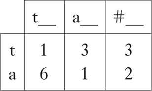
For example, the cell in the bottom left corner of this table has the value 6, because /a/ occurs after /t/ six times in the corpus. Note that although these sounds have overlapping distributions, the vectors capture the general pattern of alternation between the two. These counts can be interpreted as points or vectors in three-dimensional space, where /t/ = (1, 3, 3) and /a/ = (6, 1, 2).
4.2 What do we count when we count sounds?
The previous example counts sounds that occur immediately preceding the target sound. This is unlikely to be informative enough for anything but the simplest languages. There are many other ways we might choose to count contexts. Here I adopt a type of trigram counting that counts all contiguous triples of sounds that contain the target sound.Footnote 8 Thus our dimension labels will take the forms s 1s 2_, s 1_s₃ and _s 2s₃, where s 1, s 2, s₃ ∈ Σ ⋃ {#}.
Formally, we define an m × n matrix C, where m = |Σ| (the number of sounds in the language), and n is the number of contexts. Under the trigram contexts considered here, n = 3|Σ ⋃ {#}|2. s and c are indexes referring to a specific sound and context respectively, and each matrix cell C(s, c) is the number of times sound s occurs in context c in the corpus.
4.3 Normalised counts
Raw counts tend not to be particularly useful when dealing with vector embeddings of words, because many different types of words can occur in the same contexts (e.g. near the or is). A common technique is to normalise the counts in some way, such as by converting them to probabilities, conditional probabilities or more sophisticated measures (Jurafsky & Martin Reference Jurafsky and Martin2008). Normalisation proves to be valuable for sounds as well. Here I report results using Positive Pointwise Mutual Information (PPMI).Footnote 9
PPMI is an information-theoretic measure that reflects how frequently a sound occurs in a context compared to what we would expect if sound and context were independent (Church & Hanks Reference Church and Hanks1990). It has been used in previous models of distributional phonological learning (Silfverberg et al. Reference Silfverberg, Mao and Hulden2018). PPMI is defined in (6).
-
(6)

If P(s) and P(c) are independent, then P(s, c) ≈ P(s)P(c), and hence the value of the inner term log2 (P(s, c) / P(s)P(c)) will be close to 0. If P(s, c) occurs more frequently than the individual probabilities of s and c would predict then the value will be positive, and if (s, c) occurs less frequently than expected, it will be negative.
PPMI converts all negative values of the inner term to 0 (as opposed to Pointwise Mutual Information (PMI), which does not; Fano Reference Fano1961). This is desirable when dealing with words, because the size of the vocabulary often requires an unreasonable amount of data to distinguish between words that tend not to co-occur for principled reasons and words that happen not to co-occur in the corpus (e.g. Niwa & Nitta Reference Niwa and Nitta1994, Dagan et al. Reference Dagan, Marcus and Markovitch1995). Although this should be less of a concern with phonological data, given the relatively small number of sounds, in practice PPMI provides more interpretable results than PMI on several of the datasets examined here (see Appendix C2).Footnote 10
The three probabilities used to calculate (6) can be straightforwardly calculated from the matrix C containing phoneme/context counts using maximum likelihood estimation, as in (7).
-
(7)

We can then define a new matrix M containing our PPMI-normalised values, as in (8).
-
(8)

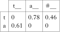
Table II shows a matrix consisting of the values from Table I converted to PPMI. The separation between the two vectors on each dimension has become even more pronounced.
Table II Count vectors for a toy language, normalised using PPMI.
5 Finding classes using Principal Component Analysis and k-means clustering
Once we have created normalised vector embeddings of the sounds in our corpus, we need a way to extract phonological classes from the space. It is intractable to consider every possible set of classes, since given an alphabet Σ, there are 2|Σ| possible classes, and hence 22|Σ| sets of classes that could be chosen. One solution is to use clustering algorithms. Broadly speaking, such algorithms attempt to assign each point in a dataset to one or more clusters, such that the points in each cluster are by some criterion more similar to other points in the cluster than to points outside of the cluster.
Many clustering algorithms with different properties and assumptions have been proposed (see Aggarwal & Reddy Reference Aggarwal and Reddy2013). The nature of the current task imposes the restrictions in (9) on the type of algorithm that should be used.
-
(9)

There are clustering algorithms that meet these criteria, particularly certain subspace clustering algorithms (Müller et al. Reference Müller, Günnemann, Assent and Seidl2009), but, for practical reasons, properties of the data considered here make them difficult to apply. First, these algorithms are generally difficult to parameterise in a principled way, requiring assumptions about the number of clusters or the distributional properties of the data. Second, traditional phonological analysis assumes that there are no outlier sounds: even if a sound is underspecified for most features (e.g. Lahiri & Marslen-Wilson Reference Lahiri and Marslen-Wilson1991), it should still belong to at least one cluster, such as the class of consonants or vowels.Footnote 11 Many common clustering algorithms assume the presence of outliers. Finally, our data consist of a small number of points, one per sound, and a large number of dimensions, one per context. Most clustering algorithms are optimised to handle the opposite situation well, and this leads to severe efficiency issues.
In light of these problems, I propose an algorithm that makes clustering well suited to this task. It works by recursively applying Principal Component Analysis and one-dimensional k-means clustering. The next sections will show that this allows for multiple partitions of the same set of sounds, while simultaneously exploiting the generally hierarchical structure of phonological classes.
5.1 Principal Component Analysis
Principal Component Analysis (PCA; Hotelling Reference Hotelling1933) is a dimensionality-reduction technique. It takes a matrix consisting of points in some number of possibly correlated dimensions and geometrically projects that data onto a set of new, uncorrelated dimensions called principal directions. These are linear combinations of the original dimensions. The dimensions of the data after they have been projected onto the principal directions are called principal components.
The number of principal components is the minimum of m − 1 and n, where m is the number of rows in the dataset and n is the original number of dimensions. Principal components are ordered descending by proportion of variance captured, with PC1 capturing the most variance, followed by PC2, and so on. This has the useful consequences in (10).
-
(10)

The mathematical details of PCA can be found in Appendix B.
PCA is useful for clustering phonological data for several reasons: first, because our matrix consists of few rows and many dimensions, its dimensions are highly correlated. Applying PCA reduces the matrix to a set of uncorrelated dimensions, which makes interpretation more straightforward. Second, PCA helps to highlight robust sources of variance while reducing noise. Finally, examining individual principal components has the potential to reveal multiple ways of partitioning a single set of sounds (see §5.2).
The generalisation performed by PCA has been achieved in various ways in previous work. Silfverberg et al. (Reference Silfverberg, Mao and Hulden2018) use PCA in an analogous way, while Calderone (Reference Calderone2009) employs independent component analysis, which is closely related. Nazarov (Reference Nazarov2014, Reference Nazarov2016) uses interaction between constraint selection and class induction to achieve a similar outcome: constraint selection chooses particular contexts to focus on, and class induction allows multiple contexts to be aggregated into a single context by inferring a phonological class.
5.2 Visualising PPMI vector embeddings of Parupa segments
A challenge in dealing with high-dimensional spaces is visualising the data. PCA proves useful for this task as well: by choosing the first two or three principal components, we can visualise the data in a way that minimises the variance that is lost. The visualisations of vector embeddings used throughout this paper will employ this technique. In addition to allowing the embeddings to be qualitatively evaluated, it also provides a partial representation of the input to the clustering component described in the next section. Note that different partitions of each set of sounds can be observed along each individual principal component.
Figure 2a shows a two-dimensional PCA visualisation of the vector space embedding of Parupa using trigram counts and PPMI weighting. The vowel/consonant distinction is clear along PC1, and vowel height is reflected in PC2.
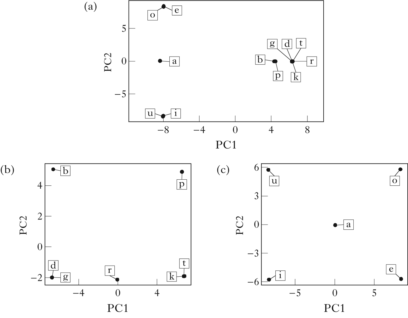
Figure 2 A PCA visualisation of the vector embeddings of Parupa, generated using trigram counts and PPMI normalisation: (a) all segments; (b) consonants; (c) vowels.
Figures 2b and 2c show PCAs generated using only rows of the matrix M corresponding to consonants and vowels respectively. For the consonants, the distinction between sounds that must precede high vowels and sounds that must precede mid vowels is reflected in PC1, while the distinction between sounds that can begin a word and sounds that cannot is reflected in PC2. For the vowels, the height distinction is reflected in PC1, while the backness distinction is reflected in PC2. Note the intermediate position of /r/ and /a/ in the plots, reflecting their shared distributions within the consonant and vowel classes.
PCA visualisations must be interpreted with caution, since they generally lose information present in the full space. In the simple case of Parupa, however, it seems clear that there should be sufficient information in the vector embeddings to retrieve the intended classes.
5.3 k-means clustering
Given a principal component, we would like to determine how many classes the distribution of sounds suggests. For example, a visual inspection of Fig. 2b suggests PC1 should be grouped into three classes: /b d g/, /r/ and /p t k/, while PC2 should be grouped into two classes: /b p/ and /d g r k t/. k-means clustering can be used to group a set of points into k clusters by assigning points to clusters in such a way that the total distance from each point to its cluster centroid is minimised (MacQueen Reference MacQueen, Le Cam and Neyman1967). That is, we assign our data points x 1 … x m to clusters c = c 1 … c k such that we minimise the within-cluster sum of squares (WCSS), as in (11).
-
(11)

where μ i is the centroid of cluster c i and ‖x − μ i‖ is the Euclidean distance between x and μ i.
In order to determine the optimal value of k, information-theoretic measures such as the Bayesian Information Criterion (Schwarz Reference Schwarz1978) can be used. Such measures attempt to strike a balance between model complexity and model fit by penalising more complex models (in this case, higher values of k), while rewarding fit to the data (in this case, distances from the cluster centroids). I use a custom Python implementation of the X-means algorithm (Pelleg & Moore Reference Pelleg and Moore2000), based on the R code provided by Wang & Song (Reference Wang and Song2011), which finds the optimal number of clusters using the Bayesian Information Criterion as an evaluation metric. When applied to PC1 and PC2 of the set of consonants discussed in the previous paragraph, this algorithm finds exactly the expected classes: namely /b d g/, /r/ and /p t k/ on PC1, and /b p/ and /d g r k t/ on PC2.
Readers familiar with clustering techniques might find it odd that clustering is carried out over single principal components rather than all dimensions, whether these be the original dimensions representing specific contexts or the reduced dimensions after PCA is performed. This is a sensible choice, because of the properties of the vector embeddings.
The columns in the vector space are massively redundant. Each principal component in a PCA can be thought of as an aggregation of the information in a correlated set of columns in the original data. Thus PCA does some of the work of finding meaningful subspaces over which clustering is likely to be effective. Each principal component can be thought of as representing some number of dimensions in the original space.
Additionally, clustering over individual principal components rather than sets of principal components allows us to find broad classes in the space that might otherwise be overlooked. This is apparent when examining Fig. 2c: clustering over PC1 and PC2 separately allows us to find distinct partitions of the vowel space based on height and backness. If PC1 and PC2 were considered together, the only likely clusterings would be either a single cluster containing all vowels, missing the class structure completely, or one cluster per sound. The latter is equivalent to finding classes that reflect the intersections of different height and backness values, but overlooks the broader class structure from which these subclasses are generated. Finding such classes is a property that many subspace clustering algorithms have, but, as described above, these algorithms are generally unsuited to this type of data. Clustering over single principal components is a simple way to achieve this property while mitigating many of the issues that arise.
Since principal components capture increasingly less and less of the total variance of the data, we may wish to cluster on only a subset of them that capture robust patterns. I return to this issue in §5.5.
The spectral clustering algorithm in Goldsmith & Xanthos (Reference Goldsmith and Xanthos2009) is similar to the method presented here, in that it clusters sounds one-dimensionally along a single eigenvector by choosing an optimal partition. Their use of maximum entropy Hidden Markov Models also involves a kind of one-dimensional clustering on emission probability ratios, setting a threshold of 0 as the boundary between clusters. Powers (Reference Powers1997) and Mirea & Bicknell (Reference Mirea and Bicknell2019) both use hierarchical clustering to extract classes from embeddings. Hierarchical clustering is simple, but not well suited to phonological class discovery: it cannot find multiple partitions of the same set of sounds, and requires the number of classes to be decided by an analyst. Finally, Nazarov (Reference Nazarov2014, Reference Nazarov2016) uses Gaussian mixture models to do one-dimensional clustering on the embeddings of segments in a context. Gaussian mixture models assume that the data was generated by some number of underlying Gaussian distributions, and attempt to learn the parameters of these distributions and provide a probabilistic assignment of points to each. This approach is perhaps the most similar to the one taken here, since k-means can be considered a special case of Gaussian mixture models that does hard cluster assignment and does not take into account the (co-)variance of its discovered clusters.
5.4 Recursively traversing the set of classes
The final component of this clustering algorithm exploits the generally hierarchical nature of phonological classes. In many cases a distinction is only relevant to segments in a particular class: for example, the feature [strident] is only relevant for coronal fricatives and affricates. Thus patterns that do not contribute a great deal to the variance of the entire set of sounds might become more apparent when only a subset of the sounds is considered. In order to exploit this hierarchical structure and detect such classes, this clustering algorithm is called recursively on the sets of classes that are discovered.
Let A be the matrix created by performing PCA on M (the matrix containing normalised embeddings of the sounds in the corpus). Suppose we perform k-means clustering on the first column of A (the first principal component of M), and discover two classes, c 1 and c 2. The recursive traversal consists of the steps in (12).
-
(12)

This process will then be repeated on c 2, on any classes discovered when clustering on A′ and on the remaining columns of A. Recursive traversal stops when (a) M′ consists of only a single row (i.e. there is a cluster containing just one sound), or (b) the clustering step produces a single cluster. Note that the original normalised embedding M is always used as the starting point: recursive traversal does not recalculate embeddings, but simply performs PCA and clustering on a subset of the rows in this matrix.
5.5 Putting it all together
To summarise, this algorithm runs Principal Component Analysis on a matrix of normalised vector embeddings of sounds, and attempts to find clusters on the most informative principal components. For each cluster found, the algorithm is recursively applied to that cluster to find additional subclusters. Considering multiple principal components for each set of sounds allows multiple partitions of these sets, and the recursive character allows it to exploit the generally hierarchical nature of phonological classes to discover more subtle class distinctions.
The steps of the algorithm and the necessary parameters are detailed in (13).
-
(13)

The two parameters that must be set here are p, the number of principal components we consider for each input, and k, the maximum number of clusters we attempt to partition each principal component into.
I choose k by assuming the typical properties of phonological feature systems, where a class is either +, ― or 0 (unspecified) for a particular feature. This suggests that we should partition each principal component into either one (no distinction), two (a +/― or +/0 distinction, as in PC2 in Fig. 2b) or three (a +/―/0 distinction, as in PC1 in Fig. 2b). Thus, setting k = 3 seems to be a principled choice.
When choosing p, we want to select only those principal components that are sufficiently informative. If p is too high, principal components that contain mostly noise will be included, and result in spurious classes being detected. If p is too low, important classes may be overlooked. There have been many proposals for how to choose the number of components (e.g. Cangelosi & Goriely Reference Cangelosi and Goriely2007). Here I use a variant of the relatively simple Kaiser stopping criterion (Kaiser Reference Kaiser1958). This takes only the principal components that account for above-average variance. This criterion is simple to calculate and works well in practice here.
In general, however, choosing how many components to use can be more of an art than a science. It is useful to consider this as a parameter that might be tuned for different purposes (for example, we might want to consider less robustly attested classes, with the intention of later evaluating them on phonetic grounds). Increasing or decreasing the number of components used has the effect of increasing or decreasing the algorithm's sensitivity to noise, and determines how robust a pattern must be to be retrieved. I will return to this point in §6.
5.6 Simplifying assumptions
I make two simplifying assumptions when applying the algorithm to the data presented in the rest of the paper: I restrict partitions of the full set of sounds to a maximum of two classes, using only the first principal component. Assuming that the most obvious partition is between consonants and vowels, this is equivalent to stipulating that the first partition of a segmental inventory must be into these two categories, and that subclasses must be contained entirely in the set of vowels or the set of consonants. This potentially misses certain classes that span both sets (like the class of [+voice] sounds, or classes containing vowels and glides, such as /i j/ and /u w/), but greatly reduces the number of classes generated, and facilitates interpretation.
Previous work has made similar assumptions about how the full set of sounds should be partitioned: spectral clustering in Goldsmith & Xanthos (Reference Goldsmith and Xanthos2009) explicitly assumes a partition into two classes when making consonant–vowel distinctions, while the maximum entropy Hidden Markov Model assumes as many classes as there are states. Studies that use hierarchical clustering (Powers Reference Powers1997, Mirea & Bicknell Reference Mirea and Bicknell2019) also implicitly make this assumption, as hierarchical clustering always performs binary splits. Thus, relative to past work, this assumption does not provide undue bias in favour of a clean consonant–vowel division.
In fact, lifting the restriction that the first principal component must be clustered into at most two classes produces different results only in the cases of Parupa and French. In both cases the full set of sounds is partitioned into three classes instead of two, and only in French are the consonant and vowel classes placed in overlapping partitions. Allowing clustering of the full set of sounds on other principal components produces additional classes in every case, but does not affect the classes that are retrieved from the first principal component. See Appendix C.3 for more discussion.
5.7 Running the algorithm on Parupa
Recursively applying PCA and k-means clustering to the Parupa vector embeddings detailed in §4 produces (14), where the classes in bold are those that might be expected from a pencil-and-paper analysis.
-
(14)

All of the expected classes indicated in Fig. 1 are present in this set. Although there are classes that do not obviously participate in the phonotactic restrictions described above, these are derivable from the expected classes: e.g. /t k d g r/ is the class of non-word-initial consonants, /d g/ is the class of non-word-initial consonants that can precede mid vowels, /t k/ is the class of non-word-initial consonants that can precede high vowels, etc. The hierarchical relationship between these classes is shown in Fig. 3, which was generated using code from Mayer & Daland (Reference Mayer and Daland2019).
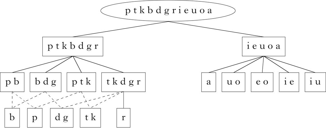
Figure 3 Classes retrieved for Parupa.
These diagrams are used throughout the paper, and do not reflect the order in which the classes were retrieved by the algorithm.Footnote 12 Rather, they arrange the classes in a hierarchical structure, where the lines between classes represent a parent–child relationship: the child class is a proper subset of the parent class, and there is no other class that intervenes between the two. Dashed lines indicate that a class is the intersection of two or more parents. These diagrams give a sense of the overall relationship between the classes retrieved by the algorithm.
Note that the singleton classes consisting of individual segments are not in general retrieved. This is the consequence of the k-means clustering component deciding that no partition of a class into two or three subclasses is justified. This is not of great concern, however, since the assumption of a segmental representation necessarily implies that singleton classes are available to the learner. These may be appended to the list of retrieved classes if desired.
This algorithm performs well on Parupa, successfully retrieving all of the intended classes, including those that involve partitioning sets of sounds in multiple ways.
5.8 Evaluating the robustness of the algorithm on Noisy Parupa
Parupa's phonotactic constraints are never violated. Although the algorithm does well on retrieving the class structure to which these constraints are sensitive, no natural language is so well behaved. In order to evaluate how well the algorithm handles noise, I examine its performance on a more unruly variant of Parupa: Noisy Parupa.
Noisy Parupa is identical to Parupa, except that some percentage of the generated word tokens are not subject to most of the phonotactic generalisations described in §3: they constitute noise with respect to these generalisations (see e.g. Archangeli et al. Reference Archangeli, Mielke, Pulleyblank, Botma and Noske2011). Noisy words still maintain a CV syllable structure, but the consonants and vowels in each position are chosen with uniform probability from the full sets of consonants and vowels. Examples of Noisy Parupa words are shown in (15), and the Hidden Markov Model for generating noisy words is shown in Appendix A.
-
(15)

A noise parameter determines what percentage of the words are noisy. Standard Parupa can be thought of as a special case, where this parameter is set to 0. As the value of this parameter increases, the algorithm should have more difficulty finding the expected classes. The model was tested on 110 corpora. The noise parameter was varied from 0% to 100% in increments of 10%, and ten corpora were generated for each parameter value.
Figure 4 shows the median number of expected and unexpected classes found by the algorithm as the percentage of noisy words increases. The expected classes are defined as exactly the classes in Fig. 1. The number of unexpected classes varies stochastically with the contents of each corpus, but the number of expected classes found remains reasonably high until 100% noise. From 40% to 70% noise, the expected classes that are not detected are either /p t k/, /b d g/ or both. In about half the cases (19/40), the unexpected classes include /p t k r/ and/or /b d g r/.Footnote 13 In 20 of the remaining 21 cases, the sets /p t/ and/or /b g/ are recovered. This indicates that the pattern is still detected to some extent, although the participating classes are less clear, due to the increase in noise.
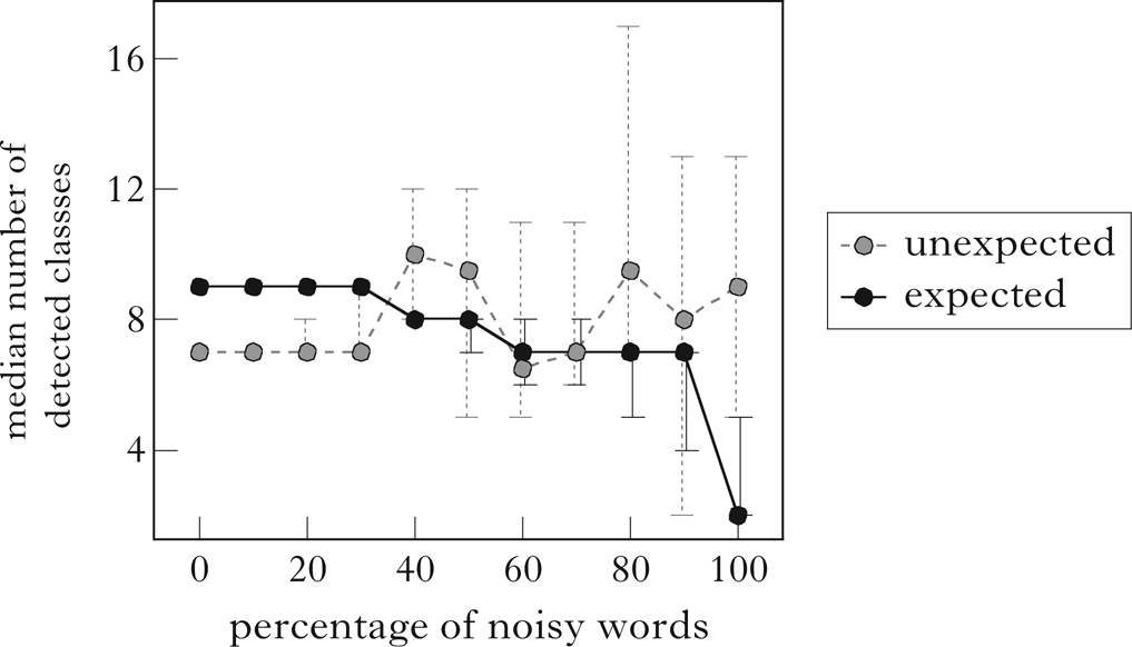
Figure 4 A plot of the median number of expected and unexpected classes found by the algorithm as the percentage of noisy words increases. Error bars span the minimum and maximum number of classes retrieved from a corpus at that noise level.
From 80% to 90% noise, the algorithm reliably fails to detect the classes /p t k/ and /b d g/, while occasionally also overlooking other classes: /p b/ (4/20), /u o/ (3/20), /i u/ (1/20), /i e/ (3/20) and /e o/ (1/20).
Finally, at 100% noise, the consonants and vowels are the only classes reflected in the distribution, and these are successfully retrieved in all cases. The other expected classes that are sometimes retrieved are the result of chance.
The results of the algorithm on Noisy Parupa suggest that it is robust to noise. All the expected classes are discovered in up to 30% noise, and even in up to 90% noise most of the expected classes are still found. Even when expected classes are lost at higher noise levels, these are often still reflected in aspects of the unexpected classes that are found.Footnote 14
6 Testing the algorithm on real language data
In this section I deploy the algorithm on several real languages: Samoan, English, French and Finnish. I include Samoan because it has a relatively small segmental inventory and fairly restrictive phonotactics, providing a simple test case. English, French and Finnish are included for continuity with previous studies (Calderone Reference Calderone2009, Goldsmith & Xanthos Reference Goldsmith and Xanthos2009, Silfverberg et al. Reference Silfverberg, Mao and Hulden2018, Mirea & Bicknell Reference Mirea and Bicknell2019). In addition to simply exploring which classes are distributionally salient in each language, my overarching goal is to successfully discover a consonant–vowel divide. More specific goals will be detailed in the relevant sections.
For these case studies, I vary the parameter that determines how many principal components of a class are considered. Recall that the default is to cluster only on principal components that account for a greater than average proportion of the variance in the data. I scale this by multiplying it by a factor (so, for example, we might only consider principal components that account for twice the average variance). This is useful because of the varying levels of distributional noise in different datasets. It is important to remember that all classes returned with a higher threshold will also be returned when the threshold is lowered, but in the latter case some additional, less robust classes will be returned as well. I vary this parameter primarily to keep the number of discovered classes suitably small for expositional purposes.The default parameter is 1. More discussion of this parameter can be found in Appendix C4.
6.1 Samoan
The Samoan corpus was generated from Milner's (Reference Milner1993) dictionary, and contains 4226 headwords.Footnote 15 The representations are orthographic, but there is a close correspondence between orthography and transcription. Symbols have been converted to IPA for clarity.
Figure 5 is a visualisation of the vector embedding of Samoan, and the retrieved classes are shown in Fig. 6. The algorithm successfully distinguishes between consonants and vowels. It also makes a rough distinction between long and short vowels, although /aː/ is grouped with the short vowels. Finally, the set of short vowels and /aː/ is split into low and non-low, while the set of long vowels is partitioned into high and mid sets. There does not appear to be a sufficient distributional basis for partitioning the set of consonants. Lowering the variance threshold for which principal components to consider did not result in more classes being learned.
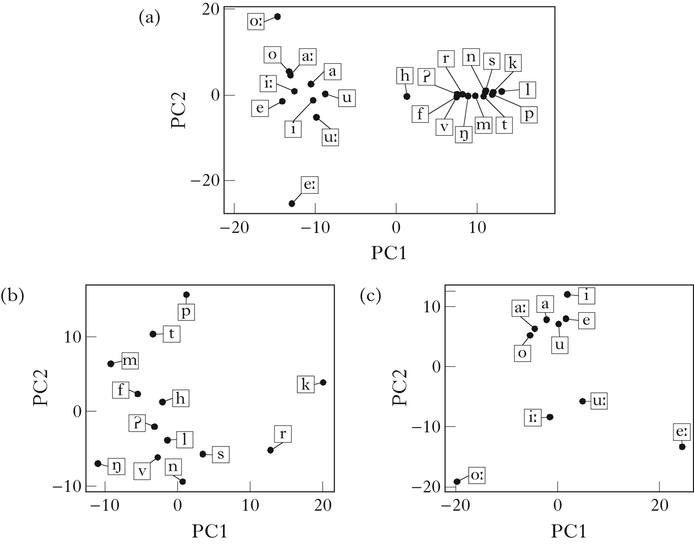
Figure 5 A PCA visualisation of the vector embeddings of Samoan: (a) all segments; (b) consonants; (c) vowels.
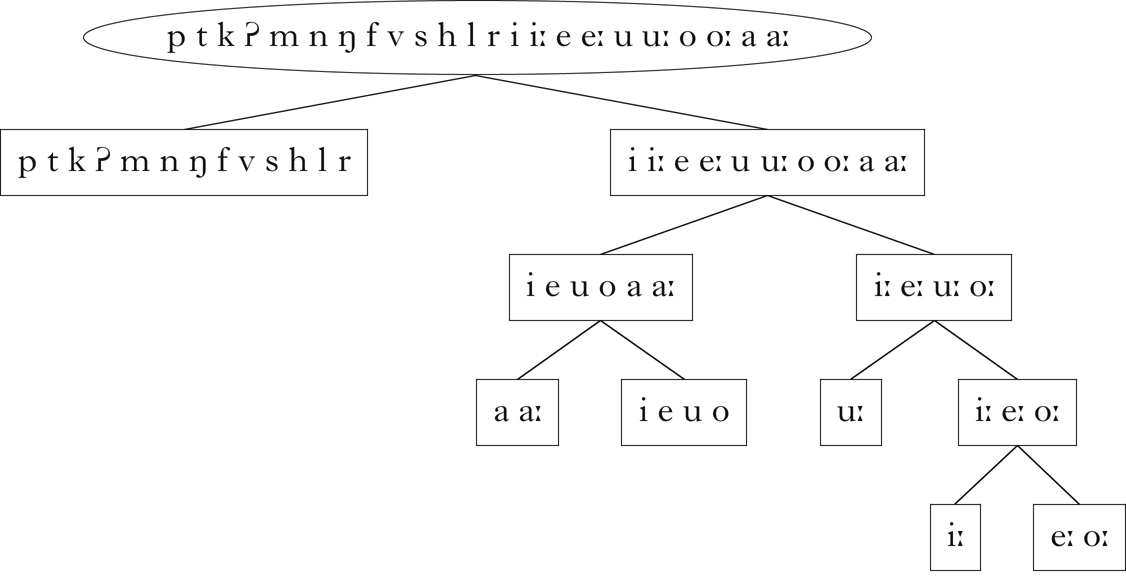
Figure 6 Classes retrieved for Samoan.
The patterning of /aː/ with the short vowels can be explained by examining its distribution. While V.V sequences are common in Samoan (1808 occurrences in the corpus), V.Vː, Vː.V and Vː.Vː sequences are rarer (226 occurrences). In 171 of these 226 occurrences, the long vowel is /aː/. Thus /aː/ patterns more like a short vowel than a long vowel with respect to its distribution in vowel sequences, and the algorithm reflects that in its discovered classes. This is an example of a class that cannot be captured using phonetic features, but is salient in the distribution of the language.Footnote 16
To examine whether the trigram window is too small to capture information that might allow the consonants to be grouped, I also ran the algorithm on Samoan with the vowels removed. This should allow it to better capture any word-level co-occurrence restrictions that might differentiate groups of consonants (McCarthy Reference McCarthy1986, Coetzee & Pater Reference Coetzee and Pater2008). A PCA of the resulting vector embedding of the Samoan consonants is shown in Fig. 7.
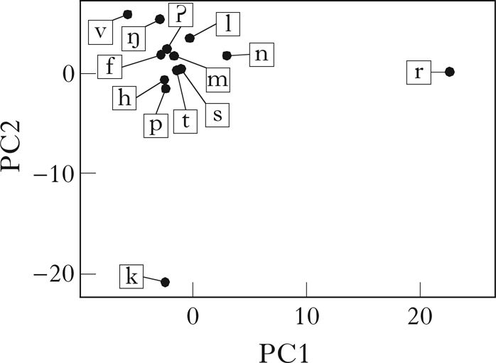
Figure 7 A PCA visualisation of the vector embeddings of Samoan consonants from a corpus without vowels (scaling factor: 1.3).
I report results from running the algorithm with a scaling factor of 1.3 on the variance threshold (i.e. only principal components with at least 1.3 times the average variance were considered). The constraint that the initial partition of the set of sounds must be binary was also removed, because the consonant–vowel distinction does not apply here. This results in the classes shown in Fig. 8. /r/ and /k/ are clearly set apart from the other consonants. These sounds are relatively uncommon in Samoan, occurring predominantly in loanwords, and this is reflected in their distribution. These sounds could be seen as distributional ‘outliers’ that are not as integrated into the phonotactics as native sounds.
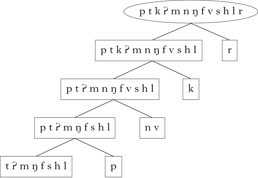
Figure 8 Classes retrieved for Samoan with no vowels.
Aside from the marginal status of /r/ and /k/ in Samoan phonology, it is hard to justify these classes in any linguistically satisfying way. The additional classes found when the variance threshold was lowered were similarly arbitrary. This suggests that consonant co-occurrence restrictions reflect little more than the special status of these consonants. Samoan has been shown to have phonotactic restrictions on root forms (e.g. Alderete & Bradshaw Reference Alderete and Bradshaw2013), and it is possible that running the algorithm on roots rather than headwords would make these patterns more detectable.
Given Samoan's strict (C)V phonotactics, it is perhaps not surprising that distribution yielded few distinctions in the set of consonants. This raises the interesting question of whether speakers of Samoan actually use phonological features to categorise consonants (other than perhaps /r/ and /k/), or if they are treated as atomic segments. I turn now to English, where the presence of consonant clusters may give us a better chance of retrieving additional phonological information.
6.2 English
The English corpus was generated from the CMU pronouncing dictionary (2008), which gives phonemic transcriptions. Only words with a frequency of at least 1 in the CELEX database (Baayen et al. Reference Baayen, Piepenbrock and Gulikers1995) were included, and some manual error correction was performed. The resulting corpus consisted of 26,552 word types. Figure 9 is a visualisation of the vector embedding of English. I report results from using a scaling factor of 1.1 on the variance threshold. The retrieved classes are shown in Fig. 10. The sets of vowels and consonants are correctly retrieved. Within the consonants, there is a distinction between /w ɹ/, /p b f h j l/ and the remaining consonants, i.e. nasals, coronal obstruents and /v/. The class of velar obstruents, /k g/, is recovered, as well as the class of labial obstruents, /p b f/, with the exception of /v/. The vowels are more difficult to interpret, but there are splits that are suggestive of the tense vs. lax distinction.
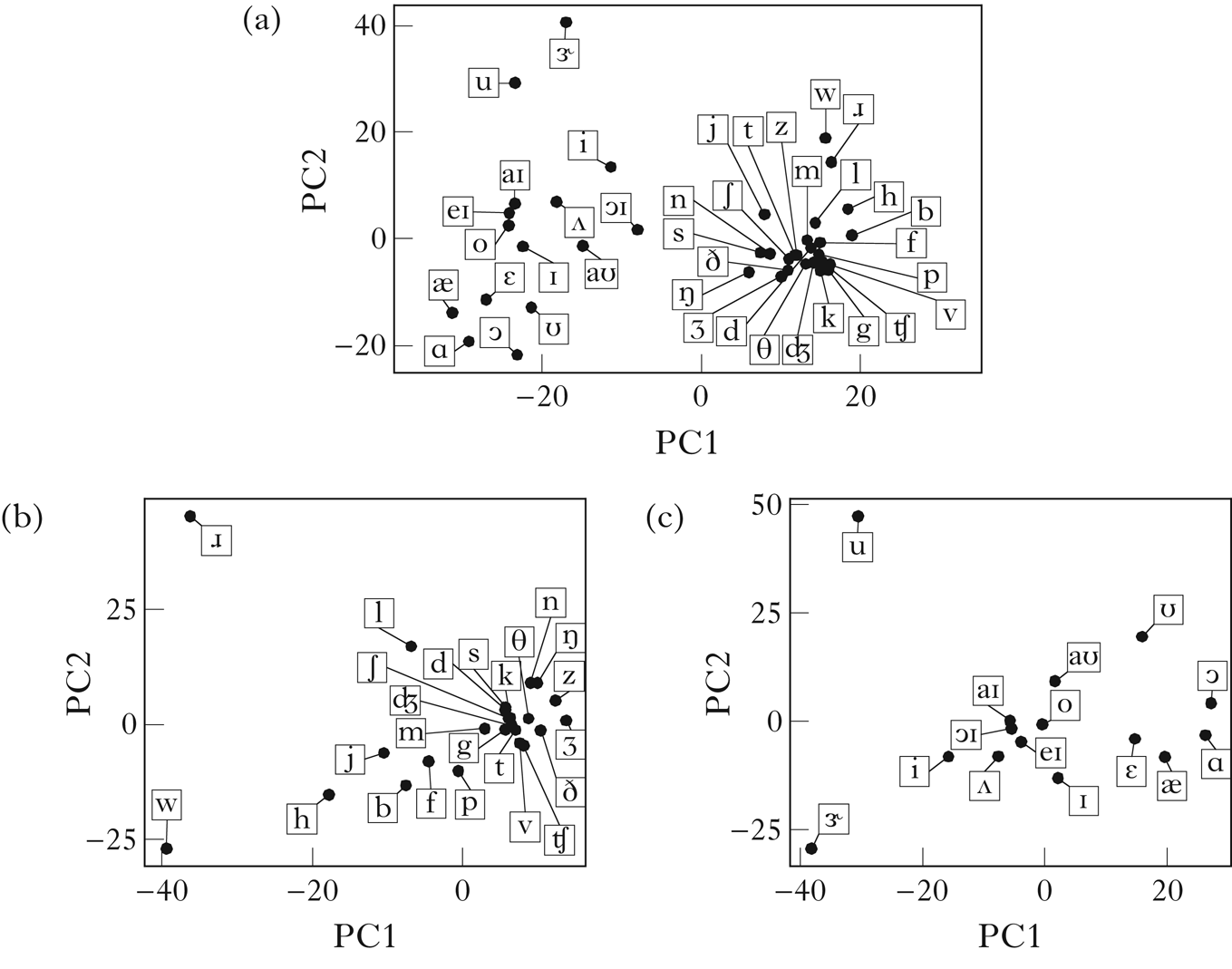
Figure 9 A PCA visualisation of the vector embeddings of English: (a) all segments; (b) consonants; (c) vowels (scaling factor: 1.1).
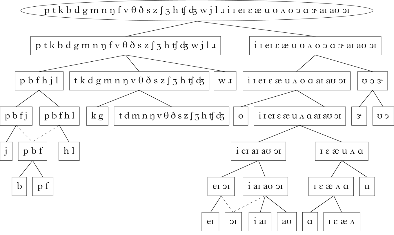
Figure 10 Classes retrieved for English.
In a language like Samoan, with a small number of sounds and restricted syllable structure, it is relatively simple to identify the specific distributional properties that lead to a particular class being detected. More phonotactically complex languages like English are not as straightforward. We can, however, get a sense of what distributional information is reflected in a principal component by looking at how contexts are linearly combined to produce that principal component. A context's coefficient in this linear combination reflects the correlation between the principal component and the context. Therefore, we can partially characterise a principal component by examining which contexts are strongly correlated with it.
There is not enough space here for a detailed exploration of the distributional properties that define each of the classes discovered here, but I will briefly look at the topmost splits within the consonant and vowel classes. As noted above, the topmost split in the consonant class is into three classes: /w ɹ/, /p b f h j l/ and the remaining consonants. This split is discovered on PC1 of the consonant embeddings, which is visible in Fig. 9b. This principal component appears to primarily capture whether segments tend to occur before or after a vowel. In the 100 most positively correlated contexts, the target consonant is followed by a vowel in 100% of contexts with a following sound (i.e. _s 2s₃ or s 1_s₃), and is preceded by a consonant or word boundary in 96% of contexts with a preceding sound (i.e. s 1_s₃ or s 1s 2_). Conversely, in the 100 most negatively correlated contexts, the target consonant is more frequently followed by a consonant or word boundary than in the highly correlated contexts (39%), and is almost always preceded by a vowel (97%). This may be interpreted as expressing a gradient preference for onset position, though the presence of /h/ in the intermediate class /p b f h j l/ indicates that this is not a complete characterisation, since this sound occurs only in onsets.
The topmost split in the vowel class is between the class /ʊ ɔ ɝ/ and the remaining vowels. This split is discovered on PC3 of the vowel embeddings, as shown in Fig. 11. This principal component appears to primarily capture how a vowel sequences with English liquids. In the 100 most positively correlated contexts, the target vowel frequently precedes /ɹ/ (54%) or /l/ (9%), but rarely follows them (/ɹ/: 3%; /l/: 2%; though it frequently follows /w/: 29%). Conversely, in the 100 most negatively correlated contexts, the target vowel frequently follows /ɹ/ (17%) and /l/ (12%), but rarely precedes them (/ɹ/: 0%; /l/: 3%). Thus, broadly speaking, this principal component appears to encode a preference for vowels to precede rather than follow liquids (particularly /ɹ/), with the class /ʊ ɔ ɝ/ tending to precede them. I leave a more detailed investigation of the distributional properties that give rise to the remaining classes as a topic for future research.
Figure 11 English vowels projected onto PC3.
6.3 French
A specific goal for the French case study is to see if the aspects of syllable structure retrieved by Goldsmith & Xanthos (Reference Goldsmith and Xanthos2009) (roughly, a distinction between vowels, onset-initial and onset-final consonants) can also be discovered using this technique. The French corpus is the one used in Goldsmith & Xanthos (Reference Goldsmith and Xanthos2009).Footnote 17 It consists of 21,768 word types in phonemic transcription. Figure 12 is a visualisation of the vector embedding of French, with a scaling factor of 1.7 on the variance threshold.Footnote 18 The retrieved classes are shown in Fig. 13. The sets of consonants and vowels are correctly retrieved. Within the consonants, there is a clean split between approximants and non-approximants, and, within the approximants, between liquids and glides. The glides are further split into rounded and unrounded glides. The vowels are more difficult to interpret, but there is a general split between nasalised vowels and vowels with unmarked roundness on one hand, and the remaining vowels on the other (/y e ə/ are the exceptions).
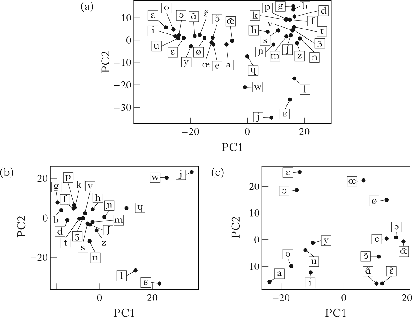
Figure 12 A PCA visualisation of the vector embeddings of French: (a) all segments; (b) consonants; (c) vowels (scaling factor: 1.7).
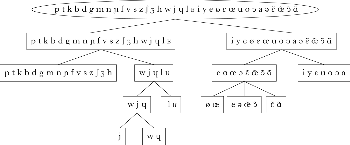
Figure 13 Classes retrieved for French.
I will again examine the distributional properties leading to the topmost splits in the consonant and vowel classes. The topmost split in the consonant class is between the set of approximants /w j ɥ l ʁ/ and the remaining consonants. This split is discovered on PC1 of the consonant embeddings, which is shown in Fig. 12b. This principal component seems to capture generalisations about syllable structure. In the 100 most positively correlated contexts, the target segment is followed by a vowel in 99% of contexts with a following sound, and preceded by a consonant in 93% of contexts with a preceding sound. The 100 most negatively correlated contexts are more likely to be followed by a consonant (43%; most commonly /l/ or /ʁ/), and are generally preceded by a vowel (89%). This appears to capture the generalisation that approximants tend to occur in complex onsets following a non-approximant. This is similar to the grouping discovered by Goldsmith & Xanthos (Reference Goldsmith and Xanthos2009) using their maximum likelihood Hidden Markov Model, although the partition here is cleaner: the class they find corresponding to onset-final segments also contains several vowels and other consonants.
The topmost split of the vowel class is between /i y ɛ u o ɔ a/ and /e ø œ ə ε̃ œ ɔ̃ ɑ̃/. This split is discovered on PC1 of the vowel embeddings, which is shown in Fig. 12c. This principal component seems to capture a tendency for vowels to be adjacent types of consonants, though it is difficult to describe succinctly. In the 100 most positively correlated contexts, the target segment is followed by a sonorant in 70% of contexts with a following sound (mostly /l/ and /ʁ/), while in the 100 most negatively correlated contexts, it is followed by an obstruent or word boundary in 91% of relevant contexts. The preceding contexts appear to differ according to place of articulation: of the 100 most positively correlated contexts, the preceding sound is coronal in 32% of relevant contexts, while in the 100 negatively correlated contexts, it is coronal in 70% of relevant contexts.
6.4 Finnish
Finnish is a central example in Goldsmith & Xanthos (Reference Goldsmith and Xanthos2009). A specific goal of this case study is to replicate their discovery of the classes relevant to vowel harmony. The Finnish vowel-harmony system is sensitive to three classes of vowels: the front harmonising vowels /y ø æ/, the back harmonising vowels /u o ɑ/ and the transparent vowels /i e/. Words tend not to contain both front and back harmonising vowels, and the transparent vowels can co-occur with either class. Goldsmith & Xanthos show that both spectral clustering and hidden Markov models are able to detect these classes (though see §7 for additional discussion).
Because the corpus used in Goldsmith & Xanthos (Reference Goldsmith and Xanthos2009) is not publicly available, I use a corpus generated from a word list published by the Institute for the Languages of Finland.Footnote 19 Finnish orthography is, with a few exceptions, basically phonemic, and so a written corpus serves as a useful approximation of a phonemic corpus. Words containing characters that are marginally attested (i.e. primarily used in recent loanwords) were excluded.Footnote 20 This resulted in the omission of 564 word types, leaving a total of 93,821 word types in the corpus. Long vowels and geminate consonants were represented as VV and CC sequences respectively.
The algorithm was first run on a modified version of the corpus containing only vowels, mirroring the corpus used in Goldsmith & Xanthos (Reference Goldsmith and Xanthos2009). The vector embedding of this corpus is shown in Fig. 14. As with the Samoan consonants, the restriction on the number of classes retrieved in the initial partition was lifted. The retrieved classes are shown in Fig. 15. The harmonic classes are successfully discovered, and, consistent with the results in Goldsmith & Xanthos (Reference Goldsmith and Xanthos2009), the transparent vowels /i e/ pattern more closely with the back vowels than with the front. In addition, classes suggestive of a low–non-low distinction are discovered among the front vowels.
Figure 14 A PCA visualisation of the vector embeddings of Finnish from a corpus with only vowels.
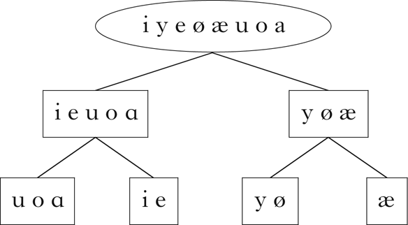
Figure 15 Classes retrieved for the Finnish corpus containing only vowels.
The algorithm was then run on the corpus containing both consonants and vowels. The vector embeddings are shown in Fig. 16, with a scaling factor of 1.2 on the variance threshold. Consonants and vowels are successfully distinguished. I focus here on the retrieved vowel classes, which are shown in Fig. 17.Footnote 21 Here the front harmonising vowels are again differentiated from the transparent and back harmonising vowels, although the split is not as clean as in the vowel-only corpus: the non-high front harmonisers /ø æ/ form their own class, and only later is /y/ split off from the remaining vowels. In addition, the distinction between transparent and back harmonising vowels is not made, although the set containing both is split into classes suggesting a high–non-high contrast. The loss of clear class distinctions when consonants are added is likely a function of the trigram counting method: because Finnish allows consonant clusters, trigrams are not able to capture as much of the vowel co-occurrence as they need to generate the expected classes (see also Mayer & Nelson Reference Mayer and Nelson2020). More will be said on this in §8.
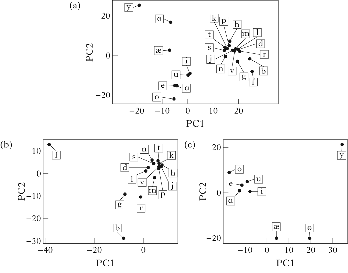
Figure 16 A PCA visualisation of the vector embeddings of Finnish: (a) all segments; (b) consonants; (c) vowel (scaling factor: 1.2).
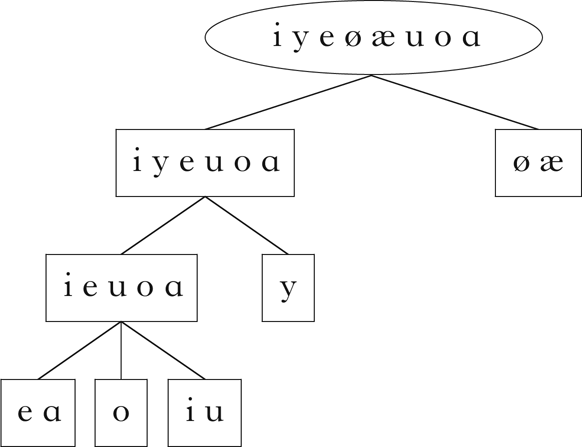
Figure 17 Vowel classes retrieved for the full Finnish corpus.
The algorithm presented here is able to retrieve the correct classes from the corpus containing only vowels, and retrieves classes that capture aspects of the harmony pattern when run on the full corpus. Although the results on the vowel-only corpus seem quite comparable to those in Goldsmith & Xanthos (Reference Goldsmith and Xanthos2009), the next section will discuss why the current results constitute an improvement in other ways.
7 Comparison with past work
A direct comparison of this algorithm to past approaches is difficult, because of the lack of a clear quantitative measure of success, the lack of publicly available implementations and the use of different datasets. Qualitative comparison is possible, however, particularly for the English, French and Finnish datasets, which are similar or identical to some of those used by previous studies (particularly Calderone Reference Calderone2009 and Goldsmith & Xanthos Reference Goldsmith and Xanthos2009). From this perspective, the current algorithm offers several notable improvements.
In none of the past approaches, with the exception of Nazarov (Reference Nazarov2014, Reference Nazarov2016), is there a clear method for producing multiple partitions of the same set of sounds (i.e. multiple class membership), or for partitioning subsets of the segmental inventory without tailoring the input to include only those subsets. The current algorithm is capable of both. Because multiple class membership and privative specification are important properties of most phonological characterisations of a language, these are desirable properties.
The spectral clustering algorithm detailed in Goldsmith & Xanthos (Reference Goldsmith and Xanthos2009) is similar to the current approach in that it decomposes a matrix representation of the distribution of sounds into a single dimension along which sounds may be clustered. There are several aspects in which the current algorithm outperforms spectral clustering. First, spectral clustering is not able to produce an accurate separation of consonants and vowels in any of the languages it has been applied to (English, French and Finnish), though Goldsmith & Xanthos suggest performance could be improved by considering a wider range of contexts. The current algorithm was able to produce this separation accurately in all cases tested here. Second, spectral clustering operates by choosing a numerical boundary between clusters that minimises conductance. The decision of how many boundaries to choose must be specified by the analyst (e.g. we choose one boundary when partitioning consonants and vowels, but two when partitioning back, front and transparent vowels). The algorithm presented here determines whether one, two or three clusters is optimal.
The maximum entropy Hidden Markov Model approach, also detailed in Goldsmith & Xanthos (Reference Goldsmith and Xanthos2009), performs better on the consonant–vowel distinction, accurately retrieving it in English and French (Finnish is not discussed). Further, it is able to identify vowel classes that participate in harmony processes in Finnish when the input consists only of vowels, and loosely captures a distinction between intervocalic and postconsonantal consonants in French. The algorithm presented here performs at least as well, and again does not require that the number of classes be specified in advance, representing a significant increase in robustness and generalisability.
The independent component analysis method described in Calderone (Reference Calderone2009) seems to be able to distinguish between consonants and vowels, as well as suggesting the existence of subclasses within these. However, Calderone does not provide a method for determining exactly how many classes are present: evidence for classes comes from inspection of visual representations of the individual components.
The algorithm presented here could be seen as a more theory-neutral variant of Nazarov (Reference Nazarov2014, Reference Nazarov2016), in that it shares components that perform similar tasks but does not assume a particular structure for the grammar. The toy language on which Nazarov's model is tested contains three phonotactic constraints that refer respectively to a single segment (no word-final /m/), one class of segments (no nasals word-initially) and two classes of segments (no labials between high vowels). Nazarov's algorithm is generally successful in learning constraints that refer to these classes, although less reliably so for the final constraint involving two interacting classes, finding it in only about half of the simulations.
When the current algorithm is run on the set of licit words in Nazarov's toy language, it successfully distinguishes between consonants and vowels, and finds the consonant classes in (16).
-
(16)

The algorithm finds classes corresponding to the labials, /p b m/, the nasals that can occur word-finally, /n ŋ/, and the nasal that cannot occur word-finally, /m/. It fails to find the full class of nasals, because it immediately partitions the set of consonants into three classes: the two nasal sets and the remaining consonants. Thus it succeeds in capturing a generalisation that Nazarov's algorithm has difficulty with (the set of labials), while not fully generalising to the nasal class, at which Nazarov's algorithm generally succeeds.
There are two additional considerations in comparing the performance of the two algorithms. First, the toy language employed has strict CVCVC candidate word forms. This is necessary to allow Nazarov's algorithm to construct a probability distribution over possible forms. Since syllable structure is pre-encoded in the candidate set, there is no opportunity for Nazarov's model to find constraints against other types of syllable structures. This means that the simulations do not test whether the learner is able to induce a consonant/vowel distinction. More generally, candidate classes must be restricted to some subset of interest, since the set of all possible words in a language is infinite. This limits the flexibility of the algorithm, since different subsets must be chosen when investigating different properties.
Second, the phonotactic constraints of the toy language are never violated. It is unclear how well Nazarov's algorithm performs on more gradient cases, which are common in natural language phonotactics (e.g. Anttila Reference Anttila2008, Coetzee & Pater Reference Coetzee and Pater2008, Albright Reference Albright2009). The algorithm presented here functions well when noise is added.
8 Discussion and conclusion
The question of what information about phonological classes can be retrieved from distributional information is of considerable interest to phonological theory. The algorithm described in this paper accurately retrieves the intended classes from an artificial language with a reasonably complex class structure, even in the presence of distributional noise. When applied to real languages, it successfully distinguishes consonants from vowels in all cases, and makes interpretable distinctions within these categories: it separates long and short vowels (with the exception of /aː/) in Samoan, captures vowel harmony in Finnish, finds classes based on syllable structure in French and English, and identifies ‘outlier’ phonemes in Samoan and Finnish.
Although the results may seem modest, they are encouraging, considering the paucity of the data. No recourse at all is made to the phonetic properties of the sounds, and the data is represented as simple strings of phonemes. Combining this algorithm with a distributional approaches to syllabification (e.g. Mayer Reference Mayer2010) and morphology (e.g. Goldsmith Reference Goldsmith, Clark, Fox and Lappin2010) would likely increase performance.
In a more fully realised model of phonological learning, a necessary subsequent step would be to derive a feature system from the learned classes. This step is not treated in this paper, but is discussed in Mayer & Daland (Reference Mayer and Daland2019), where we show that, given certain assumptions about what kinds of featurisations are allowed, an adequate feature system is derivable from a set of input classes. These two papers may be seen as complementary, and as potential components of a more realistic model of phonological learnability that takes into account other important sources of information, such as phonetic similarity (e.g. Lin Reference Lin2005, Mielke Reference Mielke2012) and alternations (e.g. Peperkamp et al. Reference Peperkamp, Le Calvez, Nadal and Dupoux2006).
An additional interesting result here is that distributional information is not equally informative for all classes across all languages. Distributional information produces an interpretable partition of vowels in Samoan, but there is little meaningful structure within the class of consonants, even when vowels are removed from the corpus. Indeed, the phonology of the language (including alternations) might not justify any such structure. French and English, on the other hand, have more interpretable results for consonants, but of the two, the result for French more closely match a typical linguistic description. This suggests that the phonotactics of any given language may refer only to a limited set of phonological classes, and, accordingly, that in some languages, phonotactics may be a stronger indicator of phonological classhood than in others.
This study suggests a variety of possibilities for future research, both in terms of improving the performance of the algorithm and of more broadly exploring the role of distributional learning in phonological acquisition.
A desirable property of the structure of the algorithm presented here is that it is modular, in the sense that the four components, vector embedding, normalisation, dimensionality reduction and clustering, are relatively independent of one another, and can in principle be modified individually (though different forms of embedding will likely require different methodologies in other components). This general structure, first quantifying similarity between sounds and subsequently using clustering to extract classes, provides a useful conceptual framework from which to approach problems of distributional learning in phonology in general, and lends itself to exploration and iterative improvement.
The counting method employed in the vector embedding step is almost certainly a limiting factor. A trigram window is small enough that long-distance dependencies may be overlooked. For the case of the artificial language Parupa, trigram counts were sufficient to capture all phonological constraints in the language, and, accordingly, the model performed well. It is likely that considering additional aspects of context would improve performance on the real languages, although simply increasing the size of the contexts considered in an n-gram model will lead to issues of data paucity. Using sequential neural networks to generate phoneme embeddings is a particularly promising possibility, since they can produce vector representations of sounds without being explicitly told which features of the context to attend to (Silfverberg et al. Reference Silfverberg, Mao and Hulden2018, Mirea & Bicknell Reference Mirea and Bicknell2019, Mayer & Nelson Reference Mayer and Nelson2020). Alternatively, integrating a mechanism for tier projection (e.g. Hayes & Wilson Reference Hayes and Wilson2008, Heinz et al. Reference Heinz, Rawal and Tanner2011) into this algorithm based on classes that have already been discovered could help mitigate the limitations of trigram counting.
An additional consideration is that this algorithm makes a fairly broad pass over the language. Meaningful distributional information about a class might be present in only very specific contexts, and this information may be indistinguishable from noise and similarly suppressed by PCA. A principled way of attending to specific contexts, perhaps along the lines of Nazarov (Reference Nazarov2014, Reference Nazarov2016), would have the potential to allow more granular classes to be revealed.
While this algorithm provides insight into what classes are apparent in language data, it does not tell us whether human learners are sensitive to this information. These questions can be explored by complementary experimental work, particularly artificial grammar learning studies (Moreton & Pater Reference Moreton and Pater2012a, Reference Moreton and Paterb).
The results in this paper show that distributional and phonetic information are often not in agreement. Given that substantive bias effects (a preference for learning phonetically coherent classes) are notoriously elusive in artificial grammar learning studies, it seems promising to further probe the hypothesis that phonological classes in real languages should be phonetically coherent. To investigate how distributional and phonetic information are integrated, researchers might perform studies that investigate whether classes that are both phonetically coherent and highly salient in the distribution of participants’ native languages are generalised more robustly in artificial grammar learning tasks than classes that are either only distributionally salient or only phonetically coherent.
In addition, it would be interesting to investigate whether distributional learning of phonological classes is a strategy available to infants (similar to word segmentation; e.g. Saffran et al. Reference Saffran, Newport and Aslin1996), or whether it is a higher-level strategy that does not become available until after further phonological development. The various assumptions and parameter values used in this algorithm (the number of partitions made, restrictions on the initial partition, the variability scalar, the order of class retrieval, etc.) may also be informed by results from acquisition studies.
Finally, as an anonymous reviewer suggests, this algorithm may have useful applications in other domains where distributional learning has been proposed, such as the learning of morphosyntactic classes (e.g. Harris Reference Harris1946).
Several current debates in phonology revolve around how great a role distributional learning plays in the acquisition and transmission of phonological structure. The algorithm presented in this paper provides some insight into what kinds of phonological information are salient in distributional data. It is my hope that this might subsequently inform further study of the extent to which human learners are able to integrate this information into their phonological grammars.


 Open access