


1. Introduction
The need for regional analysis of the impacts of climate change – in contrast to the global approach taken by Integrated Assessment Models (IAMs) such as DICE (Nordhaus and Sztorc, Reference Nordhaus and Sztorc2013; Nordhaus, Reference Nordhaus2014) – has been clearly recognized in the literature (see, for example, Easterling, Reference Easterling1997). In fact, major IAMs – such as RICE (e.g., Nordhaus, Reference Nordhaus2011), FUND (e.g., Anthoff and Tol, Reference Anthoff and Tol2013) or PAGE (e.g., Hope, Reference Hope2006) – explicitly include regional components. The regional aspects have been extended to both regional temperature effects and regional economic effects (e.g., FUND, PAGE) or to regional economic effects with predictions about mean global temperature (e.g., RICE).
Multi-region modeling in climate change economics has been developed since RICE. Desmet and Rossi-Hansberg (Reference Desmet and Rossi-Hansberg2015) developed a spatial model of climate change, Krusell and Smith (Reference Krusell and Smith2017) introduced a 20,000 region spatial model, and Hassler and Krusell (Reference Hassler and Krusell2018) discuss approaches to multi-region climate modeling. Regional aspects of climate change and associated policies have been introduced in low-dimensional IAMs in which regional temperature dynamics are driven by endogenous mechanisms of heat and precipitation transport from the Equator to the Poles (see Brock et al., Reference Brock, Engström, Grass and Xepapadeas2013, Reference Brock, Engström and Xepapadeas2014; Brock and Xepapadeas, Reference Brock and Xepapadeas2017, Reference Brock and Xepapadeas2019; Cai et al., Reference Cai, Brock, Xepapadeas and Judd2019). The climate science part of these models is based on one- or two-dimensional dynamic energy balance models, defined either in continuous space (e.g., North et al., Reference North, Cahalan and Coakely1981) or in discrete South-North ‘two-box’ models (e.g., Langen and Alexeev, Reference Langen and Alexeev2007; Alexeev and Jackson, Reference Alexeev and Jackson2013). Energy balance climate models generate spatial variability of temperature across regions through the endogenous mechanism of heat transfer. Another approach which climate science uses to generate spatial temperature variation across regions is pattern or statistical downscaling, or statistical emulation methods (see, for example, Castruccio et al., Reference Castruccio, McInerney, Stein, Liu Crouch, Jacob and Moyer2014; Hassler et al., Reference Hassler, Krusell and Smith2016; Krusell and Smith, Reference Krusell and Smith2017).
Regional temperature differentiation also emerges from the use of the transient climate response to cumulative carbon emissions (TCRE) on a regional basis. The TCRE embodies both the physical effect of CO$_{2}$ on climate and the biochemical effect of CO$_{2}$
 on the global carbon cycle (e.g., Matthews et al., Reference Matthews, Gillett, Stott and Zickfield2009, Reference Matthews, Solomon and Pierrehumbert2012; Knutti, Reference Knutti2013; Knutti and Rogelj, Reference Knutti and Rogelj2015; MacDougall et al., Reference MacDougall, Swart and Knutti2017). The TCRE, denoted by $\lambda$
 , is defined as $\lambda = {\Delta T( t) }/{CE( t) }$
 , where $CE(t)$
 denotes cumulative carbon emissions up to time $t$
 and $\Delta T( t)$
 the change in temperature during the same period. The approximate constancy of $\lambda$
 suggests an approximately linear relationship between a change in global average temperature and cumulative emissions. This roughly linear relationship has also been recognized by the IPCC (Reference Stocker, Qin, Plattner, Tignor, Allen, Boschung, Nauels, Xia, Bex and Midgley2013).
In a recent paper, Leduc et al. (Reference Leduc, Matthews and de Elía2016) identify an approximately linear relationship between cumulative CO$_{2}$ emissions and regional temperatures. This relationship is quantified by regional TCREs (RTCREs). The RTCRE parameters range from less than 1$^{\circ }$
 C per TtC for some ocean regions to 5$^{\circ }$
 C per TtC in the Arctic. Leduc et al. (Reference Leduc, Matthews and de Elía2016) consider their approach to be a novel application of pattern scaling. The high RTCRE in the Arctic is indicative of the larger anomaly at the high northern latitudes. It is understood that this anomaly could cause serious detrimental environmental effects which could be diffused to other regions south of the Arctic (IPCC, Reference Stocker, Qin, Plattner, Tignor, Allen, Boschung, Nauels, Xia, Bex and Midgley2013; Brock and Xepapadeas, Reference Brock and Xepapadeas2017). Thus one implication of adopting a regional representation of climate is that changes in the temperature in one region could generate damages in another region. It should be noted that the existence of geographical spillover damage effects across regions is supported by recent studiesFootnote 1 and that this issue could be important for policy purposes but, as far as we know, is not addressed by large-scale IAMs.
In models of climate and economy, the use of the RTCRE approach to model regional differences – rather than the structural approach based on surface albedo feedback or endogenous heat and precipitation transfer mechanisms – could provide a simplified but realistic reduced-form mechanism for modeling regional temperature dynamics.
The explicit introduction of regional temperature dynamics allows us to obtain a clearer picture of the impacts of climate change across regions, and especially across rich and poor regions. Recent literature, such as Burke et al. (Reference Burke, Hsiang and Miguel2015), Hsiang et al. (Reference Hsiang, Kopp, Jina, Rising, Delgado, Mohan, Rasmussen, Muir-Wood, Wilson, Oppenheimer, Larsen and Houser2017) and Diffenbaugh and Burke (Reference Diffenbaugh and Burke2019a), stresses that damages are larger in low latitude (warmer) areas around the Equator and are projected to become relatively larger in low latitude (warmer) areas than at temperate latitudes.
It is well-known that the study of climate change, and more specifically the economics of climate change, is characterized by fundamental uncertainties (Heal and Millner, Reference Heal and Millner2014). As Pindyck (Reference Pindyck2017) points out, we know very little or nothing about parameters or functions which are fundamental in climate change economics, such as climate sensitivity or the damage function. In the same context, Anthoff and Tol (Reference Anthoff and Tol2013) and Gillingham et al. (Reference Gillingham, Nordhaus, Anthoff, Blanford, Bosetti, Christensen, McJeon, Reilly and Sztorc2015) characterize parameters of climate–economy modeling which embody considerable uncertainties, while Lemoine (Reference Lemoine2010), Nordhaus and Moffat (Reference Nordhaus and Moffat2017), Hassler et al. (Reference Hassler, Krusell and Olovsson2018) and Cai and Lontzek (Reference Cai and Lontzek2019) discuss in detail the impacts of uncertainty on climate sensitivity. Brock and Hansen (Reference Brock and Hansen2017) distinguish three forms of uncertainty: (i) risk, which is the traditional case studied in economics in which objective or subjective probabilities are assigned to stochastic events; (ii) ambiguity, which is the case where the decision maker has concerns and is uncertain about how to weight alternative models for explaining a phenomenon, in a case where a benchmark model is ‘surrounded’ by these alternative models or probability measures; and (iii) misspecification, which is associated with the way in which we use models which are imperfect approximations of the true model.
In this paper, we refer to cases (ii) and (iii) as deep uncertainty. Since damages from climate change are projected to become relatively even larger in low latitude (warmer) areas than at temperate latitudes, it is reasonable to expect deep uncertainty to loom larger in poorer regions which tend to be lower latitude regions.
Thus the contribution of our paper is to introduce deep uncertainty and aversion to ambiguity (or concerns about model misspecification) into a multi-regional model of climate and the economy by using the robust control approach of Hansen and Sargent (e.g., Hansen and Sargent, Reference Hansen and Sargent2001; Hansen et al., Reference Hansen, Sargent, Turmuhambetova and Williams2006; Hansen and Sargent, Reference Hansen and Sargent2008).Footnote 2 Robust control methods have been applied to the economics of climate change (e.g., Hennlock, Reference Hennlock2009; Athanassoglou and Xepapadeas, Reference Athanassoglou and Xepapadeas2012; Anderson et al., Reference Anderson, Brock, Hansen and Sanstad2014). Barnett et al. (Reference Barnett, Brock and Hansen2020) explore asset pricing implications under risk and types of deep uncertainties when there are damages induced by climate change to preferences and capital accumulation. Unlike our analysis, theirs is on the planetary scale. Hence they do not analyze regional scale issues as we do here. In this literature, ambiguity or deep uncertainty was mainly associated with uncertainty of temperature dynamics or, equivalently, carbon stock dynamics. This type of deep uncertainty indirectly affects damages since the damage function depends on temperature or, equivalently, on carbon stock in the atmosphere. In the present paper, we augment the sources of uncertainty by allowing for deep uncertainty from the regulator's point of view, with regard to both regional damages and regional temperature dynamics.
However, climate and damage uncertainty is not the only source of uncertainty that we study in this paper. Recently policy makers have pointed out that climate change policy introduces transition risks, which are risks that firms will face as climate policy is introduced (e.g., Carney, Reference Carney2015), as well as physical risks, which in principle are captured by the introduction of uncertainty in temperature dynamics and the damage function. These transition risks, which are associated with changes in policy and technology, are not faced by the regulator who designs climate policy but by firms which are the subject of climate policy. In this context, we also allow for policy uncertainty and study the decisions of a robust firm which has concerns about the actual climate policy.
To summarize, the present paper contributes to climate change economics by studying climate change policies in a multi-regional model based on the novel pattern scaling approach of RTCREs under conditions of deep uncertainty associated with regional temperature dynamics, regional climate change damages, and policy in the form of carbon taxes. The paper consists of a part in which a conceptual model is developed of a social planner or regulator who maximizes global welfare in a multi-regional model under deep uncertainty, and an applied part. The applied part is based on a three-region model – the South, the Tropics and the North – with temperature dynamics characterized by RTCREs and regional damage functions. To capture the different development stages of the regions, we introduce welfare weights based on the regional GDP per capita to global GDP per capita ratio, and examine weighted and unweighted solutions.
Our results suggest that, in general, under deep uncertainty robust control policies are more conservative regarding emissions, the higher the aversion to ambiguity is, while damage uncertainty seems to produce more conservative behavior than climate dynamics uncertainty. Conservative behavior regarding emissions implies higher carbon taxes.
At the weighted – by distributional weights – solutions, carbon taxes are always relatively lower in the Tropics, which is the poorest region and bears the largest share of the global externality cost. We also show that, with the exception of the Tropics, robust climate change policies are more costly in terms of welfare relative to deterministic policy. Thus regulation when there are concerns about model misspecification and ambiguity aversion is costly. This raises the issue of learning. Thus in the final section we consider the possibility of diverting resources to learning, which will reduce concerns about model misspecification.
2. Modeling climate policy under deep uncertainty
It is clearly understood that the climate modules used in the coupled models of climate and economy, whether they are embedded in high- or low-dimensional IAMs, represent an approximation of more complex models. Therefore, in order to obtain tractability and better understanding of the basic mechanisms driving the results, we adopt the modeling approach which is based on the approximate linear relation between cumulative emissions and regional temperatures and which is quantified by the RTCREs. Having chosen an approximate model, we concentrate on deep uncertainty and concerns about model misspecification.
In the context of robust control methodology, ambiguity is introduced by allowing for a family of stochastic perturbations to a Brownian motion characterizing stochastic dynamics. The perturbations are defined in terms of measurable drift distortions. The misspecification error which expresses the decisions maker's concerns regarding departures from a benchmark model is reflected in an entropic constraint (Hansen et al., Reference Hansen, Sargent, Turmuhambetova and Williams2006; Hansen and Sargent, Reference Hansen and Sargent2008). Ambiguity and concerns about the possibility that ‘an adversarial agent’ – often referred to as ‘Nature’ – will choose not the benchmark model but another one within an entropy ball, which will harm the decision maker's objective, are reflected in a quadratic penalty term which is added to the regulator's objective. This type of ambiguity has also been referred to as model uncertainty and Hansen and Sargent call the decision maker's optimization problem with a quadratic penalty ‘the multiplier robust control problem’. A crucial parameter of the problem is the robustness parameter, which reflects the decision maker's concerns about model uncertainty or his/her aversion to ambiguity. It has been shown that as the robustness parameter, which is positive, tends to the limiting value of zero or infinity,Footnote 3 the decision problem is reduced to the standard optimization problem under risk – that is, a problem with no ambiguity aversion. When the robustness parameter increases from zero, then concerns about model uncertainty increase.Footnote 4
If the distortion of the dynamics benchmark model at time $t$ is denoted by $h_{it},$
 then the drift distortion of the stochastic dynamics is expressed by
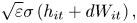
where $\sigma$ is the volatility of the stochastic dynamics, $W_{it}$
 is a Brownian motion and $\varepsilon$
 is a small noise parameter. If the term $h_{it} = 0$
 , then the problem is reduced to the case of risk. In the multiplier robust control problem (e.g., Hansen et al., Reference Hansen, Sargent, Turmuhambetova and Williams2006), the penalty associated with the distortion is expressed by

where $\theta ( \varepsilon )$ is the robustness parameter. It has been shown by Anderson et al. (Reference Anderson, Hansen and Sargent2012, Reference Anderson, Brock, Hansen and Sanstad2014) that if $\theta ( \varepsilon ) = \theta _{0}\varepsilon ,$
 then if $\varepsilon \rightarrow 0$
 , the stochastic robust control problem is reduced to a simpler ‘deterministic robust control problem’. To simplify and increase tractability, we adopt the assumption leading to a deterministic robust control problem.
To develop the climate model, we assume that the globe is divided into $i = 1,\ldots ,N$ regions. Note that Leduc et al. (Reference Leduc, Matthews and de Elía2016) divide the globe into 21 land regions. Following the RTCRE approach, regional temperature dynamics, $\dot {T}_{it}$
 , under model uncertainty can be written as

where $\mathbb {E}_{t} = \sum _{i = 1}^{N}E_{it}$ is aggregate global carbon emissions from all regions. Taking into account that a fraction of the heat stored in the atmosphere escapes, we assume that this is captured by the term $B_{i}T_{it}$
 , where $B_{i}>0$
 is the heat dissipation parameter in region $i$
 (see Nævdal and Oppenheimer, Reference Nævdal and Oppenheimer2007; Heutel et al., Reference Heutel, Moreno-Cruz and Shayegh2016; Lemoine and Rudik, Reference Lemoine and Rudik2017 ). In (3), the parameter $\sigma _{i}$
 represents volatility of regional temperature dynamics, and $h_{it}$
 the corresponding drift distortion reflecting deep uncertainty and concerns about misspecification of temperature dynamics. The initial conditions reflect that $T_{it}$
 represents the temperature anomaly relative to a given base period $T_{i0},$
 which is regarded as the initial period. We assume that concerns about regional temperature dynamics are specific for the region and, therefore, embody concerns about the RTCRE, which is also an uncertain parameter.Footnote 5
To construct the economic part of the model, we follow Brock and Xepapadeas (Reference Brock and Xepapadeas2017, Reference Brock and Xepapadeas2019) and consider a simple welfare maximization problem with logarithmic utility, where global welfare is expressed by the sum of welfare in each region and is given by:
where $y_{it}E_{it}^{\alpha }$ , $0<\alpha <1$
 , $E_{it}$
 , $T = (T_{1},\ldots ,T_{N})$
 , and $L_{it}$
 are regional output per capita, fossil fuel input or carbon emissions, temperatures in each region $i$
 at date $t,$
 and fully employed population, respectively. We assume exponential damages (see also Golosov et al., Reference Golosov, Hassler, Krusell and Tsyvinski2014)Footnote 6 and a quadratic $\psi ,$
 to allow for the possibility of increasing regional marginal damages. Thus,
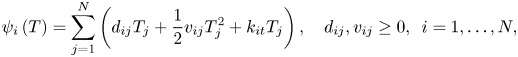
where $k_{i}$ represents ambiguity about damages in region $i$
 . Thus the damage function in region $i$
 embodies geographical damage spillovers, or cross effects, which are damages caused by temperature increases in other regions. For example, the larger anomaly at the high northern latitudes may generate damages in terms of sea level rise or greenhouse gases emitted by permafrost melting in southern regions. It is assumed that $y_{it}$
 and $L_{it}$
 are exogenously given. That is, we are abstracting away from the problem of optimally accumulating capital inputs and other inputs in order to focus on optimal emissions paths and fossil fuel taxes. In this context, $y_{it}$
 could be interpreted as the component of a Cobb-Douglas production function that embodies all other inputs along with technical change which evolves exogenously. We assume autarky for the multi-region model and no world market for loans (see also Hassler and Krusell, Reference Hassler and Krusell2012) for this approximation. Finally, $v_{i}$
 represents welfare weights associated with region $i$
 . To increase tractability, we assume that regional populations are immobile and normalized to one and define $\omega _{i} = v_{i}L_{i}$
 , $\sum _{i}\omega _{i} = 1$
 . Furthermore, to simplify the exposition even more, we assume that fossil fuels are abundant in both regions and provided at zero cost. The use of fossil fuels is, however, costly in terms of climate.
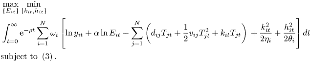
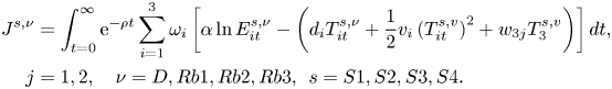
Under these assumptions, the optimization of the world's welfare which corresponds to the cooperative solution for designing climate policies can be written as
where $\omega _{i}>0 $ , $\sum _{i}\omega _{i} = 1$
 are welfare weights associated with each region. If we impose ambiguity concerns regarding damages and temperature dynamics in region $i$
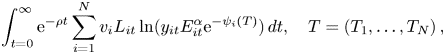
 , the cooperative solution will be the outcome of the following deterministic multiplier robust control problem:
3. Robust climate policy
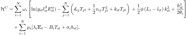
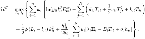
The cooperative regional climate policy emerges from the solution of problem (7). For this problem, the relevant current value Hamiltonian, after omitting the constant $\ln y_{it}$ is:
is:
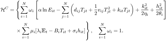
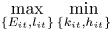
In this robust control problem, the social planner chooses regional emission paths $E_{it}$ to maximize the Hamiltonian but the adversarial agent chooses distortions $( k_{it},h_{it})$
 to minimize the Hamiltonian.
The optimality conditions for the control choices for $i = 1,\ldots ,N$ are:
are:
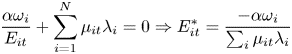


From (9), it follows that if the social planner weights all regions equally, or $\omega _{i} = \omega$ for all $i,$
 then all regions should have the same emission paths,

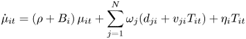
System (9)–(13), with $\mathbb {E}_{t}$ , $h_{it},k_{it}$
 substituted by their optimal values from (9)–(10), is the dynamic Hamiltonian system for the social planner. Since the robustness parameters $\{\eta _{i},\theta _{i}\}$
 reflect the ‘intensity’ of the social planner's ambiguity, the impact of deep uncertainty on optimal policy can be studied by performing comparative analysis with respect to the robustness parameters.
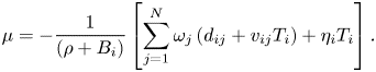
Another characteristic of the solution is that $X_{t} = \sum _{i}\mu _{it}\lambda _{i}$ is the cost of the climate externality, which consists of the sum of regional shadow temperature costs weighted by RTCREs. Thus the solution of the regional problem provides information about the contribution of each region to the global cost of the climate externality. The issue of regional contributions, which has been examined recently at the empirical level by Ricke et al. (Reference Ricke, Grouet, Caldeira and Tavoni2018), could help characterize the heterogeneity of climate impacts across the globe and provide information which could help policy design.
We examine the steady state of the cooperative solution. From (12), we obtain at a steady state:
Substituting into (13), we obtain that the steady-state regional temperatures are solutions of the system:

where

Proposition 1 If $B_{i}\neq 0$ and $\theta _{i} = 0$
 for all $i,$
 then in an open neighborhood of the point $\mathbf {o} = (v_{11},\ldots ,v_{1N},\ldots ,v_{N1},\ldots ,v_{NN},\eta _{1},\ldots ,\eta _{N}) = 0$
 , a steady state for the regional temperature anomalies which is determined by the the system (12)–(13) for $\dot {\mu }_{it} = 0,\dot {T}_{it} = 0$
 exists.
For the proof, see appendix A.
Thus it is expected that for small second-order parameters in the damage function and small robustness parameters for damages, a steady state will exist. Furthermore, at point $\mathbf {o},$ the Jacobian determinant of the linearized Hamiltonian system (12)–(13) has $N$
 negative eigenvalues $\{-B_{1},\ldots ,-B_{N}\}$
 and $N$
 positive eigenvalues $\{(\rho _{1} + B_{1}),\ldots ,(\rho _{N} + B_{N}\}$
 and therefore the steady state at $\mathbf {o}$
 has the saddle point property.
The saddle point property implies that the social planner can choose initial values and a path for regional emissions, determined by (9), so that the world economy will converge along an $N$ -dimensional manifold to the socially-optimal steady state. The paths of the costate variables $\mu _{it}$
 will determine the optimal carbon tax. The steady-state distortions $(h_{i}^{\ast },k_{i}^{\ast })$
 are obtained directly from (10) by substituting the corresponding steady states for regional temperatures and their shadow costs.
4. Optimal carbon taxes
In a global market economy, the representative ‘small’ consumer takes everything regarding climate change as fixed, beyond his/her control, and has no decision to make. The representative firm, however, does have decisions to make regarding emissions. We assume that the representative firm is subject to an emission tax or equivalently a carbon tax, and to simplify things we assume that energy has no private costs. The problem for the firm in each region is:
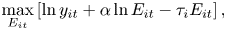
with optimality conditions
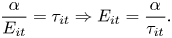
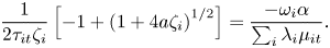
Combining (19) with (9), it follows that the optimal emission tax will be:

It is clear that unless the regulator attaches equal welfare weights to different regions, the optimal carbon tax will be different across regions. The higher the welfare weight is, the lower the optimal carbon tax for the specific region will be. If, as expected, the costates $\mu _{it}$ are negative and declining with time, the optimal carbon tax increases through time until it reaches a steady state.
Since the robust control problem is concave, the time paths of the costate variables as they converge to the steady state along the stable manifold are expected to be concave. This suggests that the optimal carbon tax will be increasing and concave. This tax, however, is expressed in terms of utils. To express it in terms of consumption at date $t$ , it should be divided by the marginal utility of consumption, which is $1/y_{it}E_{it}^{a}\exp ( -D_{i}( T_{t}) ) .$
 Since $y_{it}$
 is expected to increase over time like $\exp ( g_{i}t)$
 , this would give a convex increasing tax ramp in date $t$
 consumption units. This implies that our tax ramp is compatible in consumption units with results obtained by Nordhaus (Reference Nordhaus2014) or Golosov et al. (Reference Golosov, Hassler, Krusell and Tsyvinski2014). Furthermore, in all numerical simulations the steady-state costate values increase as the ambiguities in terms of $\eta _{i}$
 and $\theta _{i}$
 increase. Thus the optimal tax increases with ambiguity from the regulator's point of view.
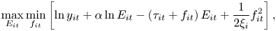
Optimal taxation of the form discussed above captures mainly physical risks and uncertainty associated with climate change as seen from the regulator's point of view. To capture policy risks and ambiguity associated with firms’ responses to climate policy, we need to introduce ambiguity aversion and preferences for robustness into the problem of the firm which maximizes profits by taking environmental policy as exogenous to the firm but uncertain. Thus we introduce policy uncertainty or ambiguity by considering the profit maximization of a firm with preferences for robustness and concerns about the size of the carbon tax which will apply to the firm's emissions under two types of robustness: (i) additive policy uncertainty, and (ii) multiplicative policy uncertainty.
Under additive policy uncertainty, the firm solves:
with optimality conditions


Taking the total differential of (23), we obtain

Thus an increase in policy uncertainty will reduce emissions for a given carbon tax.
Taking the positive root of the quadratic (23), the emissions of the robust representative firm are
Combining (25) with (9), it follows that the optimal emission tax, if the regulator takes into account the firm's concerns about policy uncertainty, is the solution of:
Under multiplicative policy uncertainty, the firm solves

with optimality conditions

Solving for $E_{it}$ , we obtain
and the optimal tax, if the regulator takes into account the firm's concerns about policy uncertainty, is the solution of
Taking the total differential of (29), we obtain

Thus, as in the case of additive uncertainty, an increase in policy uncertainty will reduce emissions for a given carbon tax.
If the regulator does not consider the possibility that the firm is concerned about policy uncertainty and sets the optimal carbon tax in the way described in the previous section, then conditions (23) or (29) suggest that the robust equilibrium for the decentralized firm is more ‘conservative’ in emissions than the robust planner. Thus, because of policy uncertainty, it may be optimal to set the tax rate a bit below the optimal Pigouvian rate.
5. Optimal robust climate policy: simulations
Although it is clear from (15) and (16) that ambiguity, misspecification concerns and regional spillovers affect steady states, emission policies and carbon taxes, the nonlinearities and the dimensionality of the problem do not allow for the derivation of tractable comparative static results. To obtain some insights into the impacts of these effects, we resort to simulations.
It should noted, however, that because of the simplicity of our model, the values obtained by our simulations should be regarded as quantitative story telling about the impacts on the optimal policies of the combined effects of deep uncertainty and misspecification concerns across regions along with regional temperature spillovers on damages. Thus our simulations depict the direction of changes on the optimal temperature anomaly paths and carbon taxes as misspecification concerns change across regions, and spillovers effects are accounted for, rather than accurate point estimates.
In designing our simulations, we chose to concentrate on a three-region model. The regions are defined as follows: R1 from 90S to 30S; R2 from 30S to 30N; and R3 from 30N to 90N. R2 contains mainly the developing world, while R3 is mainly the industrialized North. R1 is mostly ocean with parts of South America, Australia, South Africa and New Zealand. The choice of these three regions is motivated by work such as that of Burke et al. (Reference Burke, Hsiang and Miguel2015), Hsiang et al. (Reference Hsiang, Kopp, Jina, Rising, Delgado, Mohan, Rasmussen, Muir-Wood, Wilson, Oppenheimer, Larsen and Houser2017) and Diffenbaugh and Burke (Reference Diffenbaugh and Burke2019a). These studies argue that since damages are larger in low latitude (warmer) areas and are projected to become relatively even larger in low latitude areas than at temperate latitudes, it is reasonable to expect that robustness analysis of the impact of climate change on development is likely to be relatively more important for R2 than for R1 and R3. These three regions are also the focus of articles and reviews, such as Ghil and Lucarini (Reference Ghil and Lucarini2020, e.g., figures 7 and 8) or Siler et al. (Reference Siler, Roe and Armour2018), and represent regions in which climate phenomena associated with damages are different. For example, hurricanes loom much larger in [30S, 30N], and droughts and floods loom larger in the two regions outside the tropics. An additional reason for choosing them and identifying the tropical zone [30S, 30N] as a separate region is that development economists such as Sachs (Reference Sachs2001) have emphasized the problems which the tropical zone faces in doing as well economically as the temperate zones. This leads to the surmise that the tropical zone may have less adaptive capacity to cope with climate change than the temperate zones.
Recent data indicate that the regional distribution of the temperature anomaly is dominated by the larger anomaly at the high Northern latitudes, as shown in figure 1.
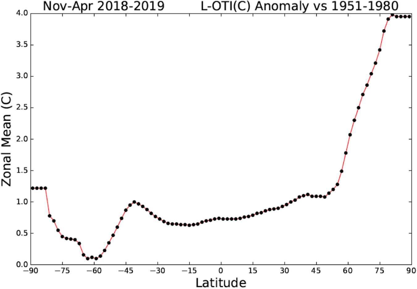
Figure 1. The temperature anomaly 90$^{\circ }$ S-90$^{\circ }$
 N.
N.
Source: GISTEMP Team, 2019: GISS Surface Temperature Analysis (GISTEMP). NASA Goddard Institute for Space Studies. Dataset accessed 25/10/2019 at data.giss.nasa.gov/gistemp/.
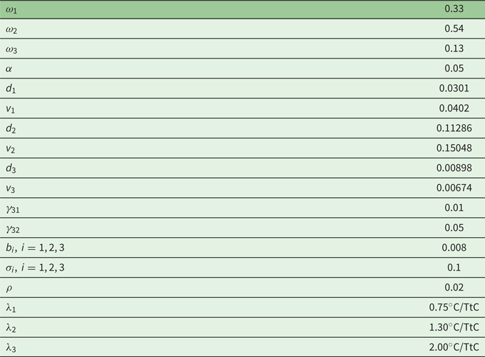
Since we are interested in exploring the impact of the larger anomaly at the high Northern latitudes, in the regional model we considered only unidirectional spatial spillovers effects due to the larger anomaly at the high Northern latitudes, from R3 to R2 and R1. Using Leduc et al. (Reference Leduc, Matthews and de Elía2016), we associated approximate RTCREs with each region. We used $RTCRE(R1) = \lambda _{1} = 0.75^{\circ }$ C/TtC, $RTCRE(R2) = \lambda _{2} = 1.3^{\circ }$
 C/TtC and $RTCRE(R3) = \lambda _{3} = 2^{\circ }$
 C/TtC. The next step was to calibrate regional damage functions.
Using data from Berkeley Earth Surface Temperatures (BEST),Footnote 7 we set approximate average annual mean land temperature for 1951–1980 at: $\textrm {R}1 \approx 15^{\circ }$ C, $\textrm {R}2 \approx 26^{\circ }$
 C, $\textrm {R}3 \approx 13^{\circ }$
 C. Then we added approximate anomalies from the NASA data –0.5$^{\circ }$
 C for $\textrm {R}1, 0.75^{\circ }$
 C for R2 and 1.25$^{\circ }$
 C for R3 – to obtain approximate regional temperatures for 2018. These temperatures are regarded as the base temperatures for calculating the optimal cooperative future regional anomalies. To calibrate a damage function of the form $\exp [d_{i}\Delta T_{i} + \frac {1}{2} v_{i}( \Delta T_{i}) ^{2} + w_{3i}\Delta T_{3}],$
 for $i = 1,2,3$
 with $w_{33} = 0,$
 we considered an average future anomaly of 3$^{\circ }$
 C which is distributed across regions in proportion to the historically-observed anomalies and added these anomalies to the average regional level temperatures calculated for 2018 to obtain regional temperatures under an average 3$^{\circ }$
 C anomaly. In Diffenbaugh and Burke (Reference Diffenbaugh and Burke2019a, supplementary information, figure S1), temperature levels are associated with damages as a proportion of GDP. Using this information, we associated average regional temperature levels calculated for the average 3$^{\circ }$
 C anomaly with the corresponding damages from Diffenbaugh and Burke (Reference Diffenbaugh and Burke2019a). This approach resulted in these approximate regional damages as proportions of GDP: $\textrm {R}1 \approx -2.5\%$
 , $\textrm {R}2 \approx -15\% $
 , $\textrm {R}3 \approx -2.0\%.$
Then the parameters of the value functions were calibrated using the relations:


where $\gamma _{i},\ i = 1,2,3$ are the damages as a proportion of GDP, and $\Delta T_{i}$
 the temperature anomalies in each region. Terms $\gamma _{31},\gamma _{32}$
 are introduced to correspond to potential impact on GDP of regions R1 and R2 respectively, due to the the larger anomaly at the high northern latitudes occurring in region R3. The terms $w_{31},w_{32}$
 correspond to the parameter of the damage function reflecting the spatial spillover effects.
Since we have no reliable information on the values $\gamma _{31},\gamma _{32}$ , we considered two scenarios. In the first – which we call ‘No spillover effects’ – it is assumed that the temperature anomaly R3 does not affect damages in the other region, or $\gamma _{31} = \gamma _{32} = w_{31} = w_{32} = 0.$
 In the second, ‘Spillover effects’, we assume that the larger anomaly at the high Northern latitudes in R3 increases damages in R2 by 1% of GDP, $\gamma _{32} = 1\%,$
 and in R3 by 0.5% of GDP, $\gamma _{31} = 0.5\%$
 . Note that these parameters are hypothetical because of the lack of relevant data. We believe, however, that the ‘Spillover effects’ scenarios could provide useful qualitative information regarding the impact of the larger anomaly at the high Northern latitudes, especially in the developing world.Footnote 8$^{,}$
 Footnote 9
The regional damage functions under the simplification implied by (33)–(35) become


Then the optimality conditions (9)–(13) become, for $i = 1,2,3,$


The optimality conditions also depend on the robustness parameters $(\theta _{i},\eta _{i})$ and the welfare weights $\omega _{i},\ i = 1,2,3$
 . In (41), the optimality condition for $k_{i}$
 indicates the maximum upwards distortion in damages which could emerge given the value of the robustness parameter $\eta _{i}$
 which reflects the planner's misspecification concerns about regional damages. If there are no concerns, $\eta _{i} = 0$
 and $k_{i} = 0,$
 but if there are concerns, then the distortion is proportional to the temperature anomaly. Therefore, for given concerns, the higher the anomaly, the higher the potential distortion in damages.
In terms of the calibration, there is no information about the possible value of the misspecification concerns that a planner might have regarding regional damage function and temperature dynamics. We know, however, from studies such as Burke et al. (Reference Burke, Hsiang and Miguel2015), Hsiang et al. (Reference Hsiang, Kopp, Jina, Rising, Delgado, Mohan, Rasmussen, Muir-Wood, Wilson, Oppenheimer, Larsen and Houser2017) and Diffenbaugh and Burke (Reference Diffenbaugh and Burke2019a), that damages are larger in low latitude (warmer) areas and are projected to become relatively even larger in low latitude areas than at temperate latitudes. Hsiang et al. (Reference Hsiang, Kopp, Jina, Rising, Delgado, Mohan, Rasmussen, Muir-Wood, Wilson, Oppenheimer, Larsen and Houser2017) project larger damages for lower latitudes even for an advanced country like the U.S. This suggests that it would be reasonable to stratify the planner's problem with misspecification concerns about damages that increase as the latitude gets closer to the Equator because of lack of understanding of the inefficiencies of adaptive response to climate change which is increasing as the latitude gets closer to the Equator. This could be attributed to the lack of understanding of the inefficiencies of adaptive response to climate change which is a given part of ‘technology’ and includes limits on adaptive capacity. The lack of understanding increases as we move towards the Tropics, along with the ambiguity associated with the large heterogeneities of the returns to factors of production in developing countries (our Tropics region R2) relative to developed countries.Footnote 10 This implies that $\theta _{2}$ should be greater than $\theta _{1}$
 and $\theta _{3}.$
Furthermore, given the uncertainties associated with the larger anomaly at the high Northern latitudes, it might be reasonable to assume that the planner might have stronger misspecification concerns about temperature dynamics in region R3, the North. This implies that $\eta _{3}$ should be greater than $\eta _{1}$
 and $\eta _{2}.$
The spatial structure of the models and the associated differences in the average development stage of each region implies that there should be differentiation among welfare weights. We followed the cost benefit analysis literature (e.g., OECD, 2018, chapter 11) in defining distributional weights as

where $\bar {y}$ is world GDP per capita, $y_{i}$
 is GDP per capita in region $i,$
 and $e$
 is the elasticity of marginal utility. We use $e = 1$
 to be compatible with our assumption about logarithmic utility. Using World Bank data for GDP per capita in 2018, we obtain $\hat {\omega }_{i}$
 and then we normalize them to $\omega _{i}{:}\ \sum _{i = 1}^{3}\omega _{i} = 1.$
 By associating R1, R2 and R3 with GDP per capita of upper middle income countries, low and middle income countries, and high income countries respectively, the values of the welfare weights obtained are:

5.1. Simulation results
To study the differentiation of optimal robust policies when misspecification concerns and welfare weights differ across regions, we consider the following four simulation scenarios:
1. S1: No spillover effects and equal welfare weights.
2. S2: No spillover effects and unequal welfare weights.
3. S3: Spillover effects and equal welfare weights.
4. S4: Spillover effects and unequal welfare weights.
In each scenario, we consider four cases:
(a) D: No misspecification concerns, $\theta _{i} = 0,\eta _{i} = 0 $
 , $i = 1,2,3$. This is the deterministic case.
(b) Rb1: Robust control with $\theta _{2} = 1 $
, $\theta _{1} = \theta _{3} = 0,\eta _{3} = 0.5 $, $\eta _{1} = \eta _{2} = 0.$(c) Rb2: Robust control with $\theta _{2} = 2 $
, $\theta _{1} = \theta _{3} = 0,\eta _{3} = 0.75 $, $\eta _{1} = \eta _{2} = 0.$(d) Rb3: Robust control with $\theta _{2} = 3 $
, $\theta _{1} = \theta _{3} = 0,\eta _{3} = 1.0 $, $\eta _{1} = \eta _{2} = 0.$


Cases Rb1, Rb2 and Rb3 capture the notion of higher concerns about damages in the Tropics and higher concerns about temperature dynamics in the North. Misspecification concerns increase as we move from Rb1 to Rb3.
In the simulations, we first obtain numerical solutions for the steady state of the nonlinear system (40)–(45). This corresponds to a steady state for the temperature anomalies and the corresponding shadow cost for the anomaly – that is, the costate variable – in each region. Then the Hamiltonian system (42)–(45) is linearized at the steady state and its Jacobian matrix is calculated. It is verified that this matrix has three negative and three positive eigenvalues; therefore the steady state is a saddle point, and transversality conditions at infinity are satisfied. The system of the six linear ordinary differential equations (ODEs) resulting from the linearization of (42)–(45) is solved with initial values for the temperature anomalies and terminal values for the steady-state vector, by setting the constants corresponding to positive eigenvalues equal to zero. This allows us to obtain the optimal transition paths toward the steady state in the neighborhood of the steady state. In figure 2 we present the paths for optimal anomalies (left panel) and emissions (right panel) resulting from the solution of the linearized Hamiltonian system, for scenario S4, Rb1. The paths for all the rest of the cases are similar, with convergence to different steady states.
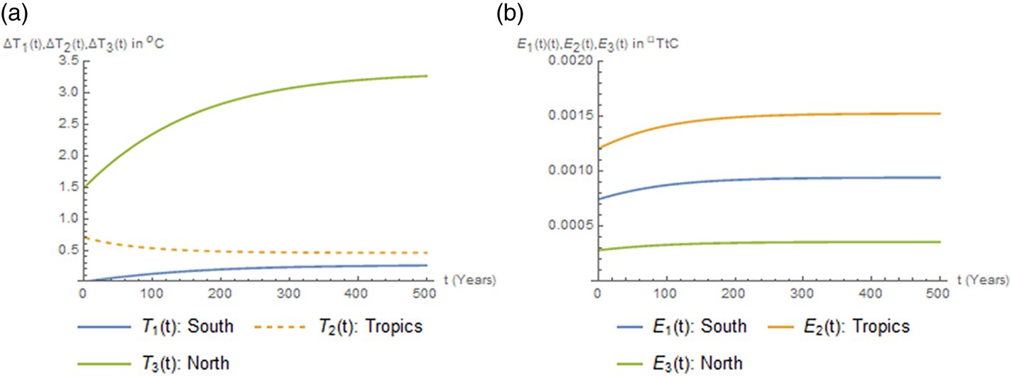
Figure 2. Paths for optimal temperature anomalies (left panel) and emissions (right panel) for scenario S4, Rb1.
In table 1, we present simulation results regarding optimal steady-state anomalies, optimal steady-state taxes as defined in (20), for steady-state values $\mu _{i}^{\ast }$ , and the proportion of the global cost of climate externality attributed to each region defined as $X_{i} = (\lambda _{i}\mu _{i}^{\ast }) \diagup (\sum _{i}\lambda _{i}\mu _{i}^{\ast }) $
 , $i = 1,2,3$
 . The steady-state anomalies $\Delta T_{i}$
 are expressed in $^{\circ }$
 C, while the taxes are presented as an index in which the scenario S1, D, which is a deterministic case without spillover effects and region-specific distributions weights – the scenario most analyzed in low-dimensional climate models – is regarded as the base.Footnote 11
Table 1. S1–S4: No spillover effects and (a) equal welfare weights, (b) region-specific welfare weights, (c) equal welfare weights and (d) region-specific welfare weights
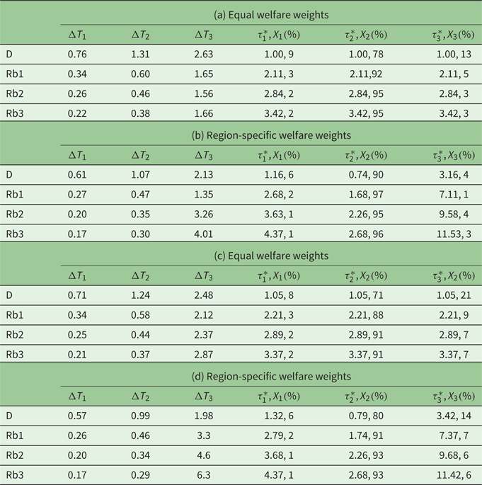
The simulation results suggest the following:
• Increase in preferences for robustness, or misspecification concerns, reduces emissions in all regions.
• Increase in preferences for robustness reduces temperature anomalies in the South and the Tropics, but not in the North. This can be justified in the following way. We run a large number of simulations which indicated that under robust control, and provided that the worst scenario emerges, increasing the $\theta$
–$\text {ambiguity}$ with no $\eta$–$\text {ambiguity}$ leads to higher steady-state emissions, because the choice of the adversarial agent is equivalent to increasing the impact of emissions on the change in temperature. In this case, the planner's policy is to reduce emissions and increase the carbon tax, but the distortion which increases the temperature rate of growth eventually leads to a relatively higher steady-state anomaly relative to the no ambiguity case. Since in our simulations temperature dynamics misspecification affected only the North, the anomaly increases only there, despite the fact that the North's emissions are reduced. On the other hand, increasing $\eta$–$\text {ambiguity}$ with no $\theta$–$\text {ambiguity}$ leads to lower steady-state temperatures under robust control. When both types of ambiguity exist, as in the case of table 1, there are two opposite impacts on steady-state anomalies and the final outcome will depend on the relative strength of the effects. In the cases reported in table 1, the $\theta$–ambiguity effect dominates when the $\theta$–ambiguity is more than Rb2 and in some cases more than Rb1 and, therefore, the temperature anomaly in the North increases.• Increase in preferences for robustness uniformly increases the optimal robust carbon tax relative to the benchmark case of no ambiguity and equal welfare weights (S1D), when welfare weights are equal.
• Increase in preferences for robustness, with unequal welfare weights, uniformly increases the optimal robust carbon tax relative to the benchmark case of no ambiguity and equal welfare weights (S1D), but the carbon tax for the Tropics is always lower than the tax for the South and the North. The tax for the North is always the highest. This result is in line with the report by the High-Level Commission on Carbon Prices (2017), and Reference StiglitzStiglitz's (Reference Stiglitz2019) recommendations of nonuniform carbon taxes, with carbon taxes being relatively higher in regions where consumers are disproportionally rich. Brock et al. (Reference Brock, Engström and Xepapadeas2014), in a continuous space model with heat transport Polarwards, also show that optimal carbon taxes are higher in relatively richer regions in which the marginal utility of consumption is lower.
• The proportion of the global cost of climate externality attributed to each region $( X\%)$
is always the highest in the Tropics and increases with unequal welfare weights and misspecification concerns.Regarding the choice of the damage function, we understand that there are controversies around the empirical papers we use to calibrate our damage function. For example, Rosen (Reference Rosen2019) argues that the temperature estimates in Diffenbaugh and Burke (Reference Diffenbaugh and Burke2019a) are biased upward and their regression analysis is flawed because of omitted variable bias.Footnote 12 While it is beyond the scope of this paper to deal with this debate, it is suggestive of a rather large layer of uncertainty surrounding the three damage functions in our formulation. The extensive discussions and the controversies associated with the damage function (e.g., Pindyck, Reference Pindyck2017) and, more specifically for our case, the controversy between Diffenbaugh and Burke (Reference Diffenbaugh and Burke2019a) and Rosen (Reference Rosen2019) – since we use Diffenbaugh and Burke (Reference Diffenbaugh and Burke2019a) for our calibrations – is a good reason to use alternative damage functions in a robustness analysis.
We thus performed sensitivity analysis by uniformly reducing the coefficients of the quadratic formulations (37)–(39) and by using a linear version by setting $v_{i} = 0 $
, $i = 1,2,3.$ In all simulations the qualitative structure of the results remains the same as our central results presented in table 1. The linear formulation of the damage function leads to higher steady-state temperatures for all three regions, but the qualitative behavior remains the same as with the quadratic specification. More specifically, with a linear damage formulation the steady-state anomalies corresponding to row D of table 1 are $(\Delta T_{1},\Delta T_{2},\Delta T_{3}) = ( 1.62,2.81,5.62),$ while the steady-state anomalies corresponding to row D of table 1 are $(\Delta T_{1},\Delta T_{2},\Delta T_{3}) = (2.04,3.54,7.08),$ which suggests that the specification of the damage function, and for our case the existence or not of strict convexity, is important in determining the socially-optimal steady-state levels and the paths to the steady state. The debate over specifying a realistic damage function is an open issue in climate change economics.Footnote 13


6. The welfare impact of robustness
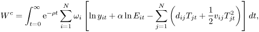
An issue which arises when a robust climate policy is pursued is whether the policy incurs additional welfare costs or benefits relative to the case in which no misspecification concerns are involved.Footnote 14 To obtain an approximation of these costs, we calculate the global welfare indicator:
The indicator corresponds to the case in which the global regulator is committed to the emissions paths obtained through the relevant robust control optimizations. The indicators were calculated numerically and the results are shown in figure 3.
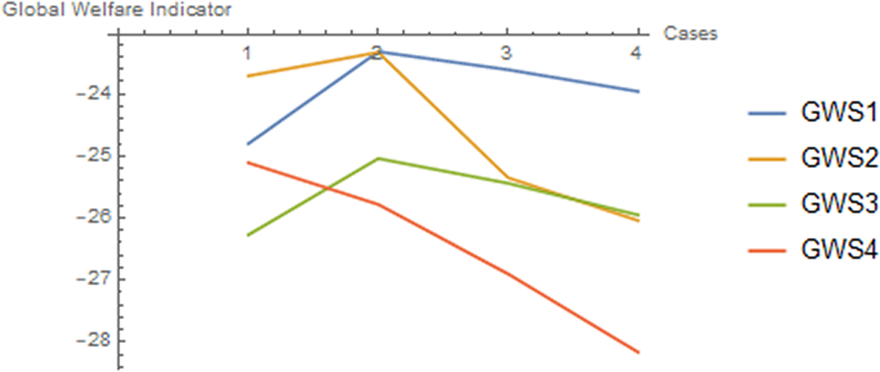
Figure 3. Evolution of global welfare indicators (GW) for S1, …, S4 when preferences for robustness increase.
Note: On the horizontal axis, 1 is D, 2 is Rb1, 3 is Rb2 and 4 is Rb3.
The results indicate that, with the exception of S4, welfare increases as the planner has mild concerns about misspecification (case Rb1). Then, as misspecification concerns become stronger, welfare is decreasing. This means that in Rb1 the global gains from reducing emissions and global warming counterbalance the loss in terms of output due to the lower emissions. As misspecification concerns increase, the output effect becomes stronger and welfare is reduced. Therefore, for a given low level of aversion to ambiguity by the planner, robust policy could be welfare enhancing at the global level. For high aversion, our numerical results indicate that robust policies have a welfare cost.
It will be interesting to examine this global result in terms of the impact of robust control on individual regional welfare. In this case, the welfare indicator will be:
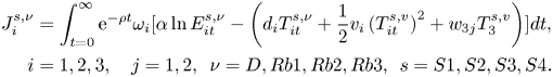
The simulation results are shown in figure 4.
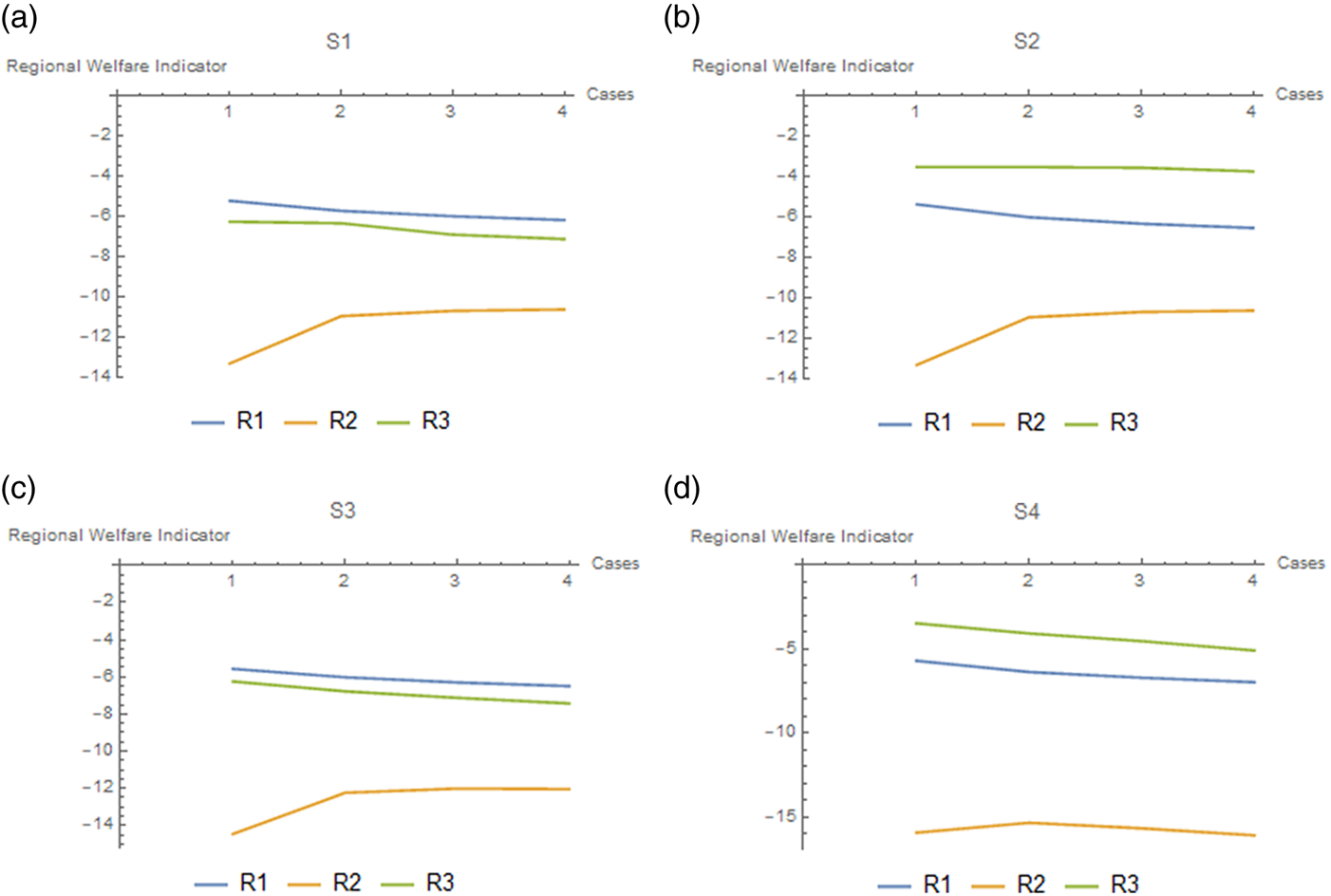
Figure 4. Evolution of regional welfare indicators when preferences for robustness increase.
Note: On the horizontal axis, 1 is D, 2 is Rb1, 3 is Rb2 and 4 is Rb3.
The results suggest that robust control at the global level is beneficial for the Tropics only. The reason is that since global emissions are reduced by robust control, and the Tropics suffer most of the damages, the gain for this region from the reduction in climate change damages exceeds the losses from reduced output.
7. Learning and robust control
The numerical results of the previous section indicate that robustness could be costly, relative to the case of no concerns about model misspecification, especially in the cooperative solution. This raises the issue of whether it is possible to avoid this cost by learning. In Anderson et al. (Reference Anderson, Hansen and Sargent1998: 2), it is stated that ‘Superficially at least, the perspective of the ‘robust’ controller differs substantially from that of a ‘learner”. In our dynamic settings, the robust decision maker accepts the presence of model misspecification as a permanent state of affairs, and devotes his/her thoughts to designing robust controls, rather than, say, thinking about recursive ways to use data to improve the model specification over time. The idea here is that the ‘learner’ cannot improve against model misspecification even with a large amount of data.
However, when dealing with climate change issues, the stakes are high and learning through scientific research is an ongoing process which might remove some concerns regarding damages or temperature dynamics. To model such a process, we consider the case in which part of the labor force, which in the model without learning is fully employed in the output producing sector, could be employed in the ‘learning’ sector. Employment in the learning sector reduces misspecification concerns, since it allows the regulator to learn about the processes for which there is ambiguity. We assume that the robustness parameter can be expressed as the function:

where $l_{it}$ is labor input used in region $i$
 to produce output at time $t,$
 and $L_{i}-l_{it}$
 is labor input allocated to the learning sector for climate damages. Assume that learning activities take place only with respect to damages from climate change and that the world is changing rapidly so that no learning stock is accumulated.Footnote 15 The regulator's objective associated with the multiplier representation of the robust control problem can be written as:

subject to (3). For this problem, the current value Hamiltonian is:
Optimality conditions for $i = 1,\ldots ,N$ imply:


This formulation implies that learning about climate damages from the regulator's point of view raises the cost of the ‘adversarial agent’ who tries to minimize the regulator's welfare. Since $\phi ^{\prime }>0$ , an increase in the amount of labor allocated to learning will reduce the penalty that the adversarial agent could impose on the regulator. To put it differently, an increase in learning reduces misspecification concerns and ambiguity. Under this setup, the following result can be stated.
Proposition 2 An increase in the regional temperature will always increase the labor input allocated to the learning sector.
For the proof, see appendix A.
Similar to condition (41), condition (52) shows that the maximum distortion of damages due to misspecification concerns is proportional to the temperature anomaly with proportionality coefficient $1/\phi ( L_{i}-l_{it}).$ This proportionality coefficient depends on labor allocation. Our proposition indicates that if the temperature anomaly increases, the planner has an incentive to increase labor input allocated to learning. By doing so, the regulator can reduce his/her concerns about misspecification, which means that the maximum damage distortion according to which the regulator has to design emission policy is lower. This implies more emissions along the optimal path. Allowing more emissions, because of the lower damage distortion, will increase output. Of course there is a trade-off here since, by allocating more labor to the learning sector, there will be a negative impact on output. These trade-offs are captured by the optimal solution.
Other generalizations are also possible. One approach could be to consider allocation of labor across three activities: production of goods; mitigation of damages, that is, adaptation to climate change; and our type of ‘learning’. In the optimal allocation of labor across these three activities by a Pareto optimal planner, it could be possible to locate plausible sufficient conditions for a positive amount of labor to be allocated to all three activities, e.g., Inada type conditions. Furthermore, in a competitive model the wage rate of labor in each region could increase as the demand for labor increases due to increased labor demand for adaptation. A possible way of generalizing to a model with three labor activities is to make the damage parameters in equations (4) and (5) a function of labor allocated to damage mitigation. This means defining the damage parameters as $d_{ij}(l_{ij})$ where $l_{ij}$
 is labor allocated to damage mitigation. As this type of labor increases, $d_{ij}$
 decreases. If we assume that $d_{ij}(0)>0,d_{ij}^{\prime }(0)\ll 0$
 and $d_{ij}^{\prime }(\infty ) = 0$
 while $d_{ij}^{\prime }( l_{ij}) <0$
 for all $l_{ij},$
 along with $d_{ij}^{\prime \prime }( l_{ij}) >0$
 and $d_{ij}^{\prime }(0) = -\infty$
 for an Inada condition, the maximizing agent's problem (the social planner's problem) is concave and the minimizing agent's problem is convex; therefore some labor should be allocated to mitigating damages. The full analysis of such a problem is outside the objective of the current paper, but it represents an interesting area of further research, since much attention has been given recently to the mitigation of damages from climate change, that is, adaptation.
8. Concluding remarks
Deep uncertainties are associated with both the natural and the economic characteristics of climate change. These uncertainties are amplified by the fact that in reality the temperature anomaly evolves differently across the globe, with a faster increase in the area of the North Pole relative to the Equator, because of natural mechanisms. In this context, we study climate change policies by using the novel pattern scaling approach of RTCREs and develop an economy–climate model under conditions of deep uncertainty associated with temperature dynamics, regional climate change damages, and policy in the form of carbon taxes. The regional structure of the model allows us to analyze the distributional effects of climate change on regional carbon taxes.
We applied robust control methods to derive optimal emission policies and the associated price of the climate externality and carbon taxes under the different sources of deep uncertainty. Our results indicate that in general robust policies under deep uncertainty lead to more conservative emission policies relative to a deterministic situation. Furthermore, ambiguity related to the damage function tends to produce more conservative policies than ambiguity in temperature dynamics, while robust control with high concerns about model misspecification is relatively more costly, but this could depend on the vulnerability of a region in noncooperative solutions. The most vulnerable region in our parametrization benefits in welfare terms from robust policies when misspecification concerns are mild. Furthermore, the most vulnerable/poorest region pays a lower carbon tax when distribution across regions is taken into account. We also show that competitive firms, when facing ambiguity regarding carbon taxes, tend to be more conservative and use smaller amounts of fossil fuels relative to the case of no policy uncertainty. Policy uncertainty could be important in practice because it relates to uncertainties in the transition to a low carbon economy.
Our results suggest that in the context of the Paris accord (COP 21) and the further development of the ‘Paris rulebook’, it will be important to address the need to differentiate policy instruments, either as carbon taxes or tradable permits, among rich and poor countries and the potential issues associated with the emergence of carbon leakage.
Future research is needed that focuses on impacts of climate change on the pricing of regional assets and the pricing of uncertainties impacting such assets. At the global scale, Barnett et al. (Reference Barnett, Brock and Hansen2020) have made progress on pricing a trinity of uncertainties, i.e., risk, ambiguity aversion and misspecification uncertainties. At latitude-specific regional scales, based upon the work of Burke et al. (Reference Burke, Hsiang and Miguel2015), Hsiang et al. (Reference Hsiang, Kopp, Jina, Rising, Delgado, Mohan, Rasmussen, Muir-Wood, Wilson, Oppenheimer, Larsen and Houser2017) and Diffenbaugh and Burke (Reference Diffenbaugh and Burke2019a), it is plausible to speculate that all three of the trinity of uncertainties are likely to grow relatively larger at lower latitudes compared to higher temperate latitudes in future projections of climate impacts. Such impacts on assets plus the concern about ‘stranded assets’ (e.g., Barnett, Reference Barnett2019) and potential impacts of climate change on monetary policy (Economides and Xepapadeas, Reference Economides and Xepapadeas2018; San Francisco Federal Reserve Bank, 2019) suggest that research on pricing latitude-specific regional asset uncertainties is an important area for future research.
Another line of research could focus on strategic interactions among regions, in a set-up in which a cooperative solution cannot be attained and, as a result, each regional planner maximizes own welfare by taking into account own misspecification concerns and takes the emission paths and the misspecification concerns of the other regions as given. Brock and Xepapadeas (Reference Brock and Xepapadeas2019) studied this problem in a deterministic set-up. It would undoubtedly be interesting to study how differences in misspecification concerns would affect the open loop or feedback Nash equilibrium.Footnote 16 Although the solution of this problem is beyond the objectives of this paper, its solution would reveal the impact of the interactions between regions exhibiting strategic behavior under deep uncertainty which has a spatial structure, since misspecification concerns are expected to be different across regions.
Acknowledgments
We are grateful to two anonymous referees for valuable comments and suggestions on an earlier draft of this paper. William Brock thanks RDCEP (Robust Decision Making on Climate and Energy Policy) at the University of Chicago under National Science Foundation grants SES-0951576 and SES-1463644 for support of some of his work cited in this article. Anastasios Xepapadeas thanks the AUEB Research Center Program 3049-01 for support of this work. None of the above are responsible for any errors or shortcomings in this article. The authors gratefully acknowledge technical editing assistance from Joan Stefan.
Appendix A:
Proof of Proposition 1: The proof follows directly from the application of the implicit function theorem. The system (12)–(13) has a straightforward solution at point $\mathbf {o},$

and the Jacobian determinant of (12)–(13) is nonzero at $\mathbf {o}.$
Proof of Proposition 2: If we substitute the minimizer for $k_{it}$ from the optimality conditions (50)–(54), the reduced form Hamiltonian becomes:
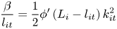
The optimal choice for the labor input is given by

Assuming that the learning function can be specified as $\phi (l) = ( A/q) l^{q}$ , we obtain

which implies that the optimal allocation of labor to production and learning is a function of temperature. Implicit differentiation results in
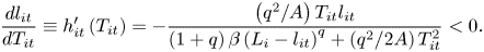
Thus an increase in temperature in region $i$ will reduce the labor input to production and increase the labor input allocated to learning and to reducing ambiguity about climate change damages.
Appendix B:
The parameter values used in simulations are shown in table B1.
Table B1. Simulation parameters


 Open access