


1. Introduction
With the advent of satellite mega-constellations, the density of objects in low Earth orbit (LEO) is predicted to reach 0.005–0.01 objects per degree square (McDowell Reference McDowell2020). Most of the current space surveillance radar systems dedicated to monitoring such objects in space (Space Domain Awareness: SDAFootnote a) operate at VHF/UHF/S-Band and utilise active transmitters to reflect signals from objects in the space environment (Goldstein, Goldstein, & Kessler Reference Goldstein, Goldstein and Kessler1998). The predicted increase in the density of LEO objects demands detection systems with large instantaneous field-of-view (FOV) receivers, the ability to change pointing directions and tracking quickly, and wide field illuminators. We aim to address these issues by using the Murchison widefield array (MWA) as a sensitive passive receiver in the FM band, coupled with existing, uncoordinated FM transmitters as the illuminators.
Previously, Prabu et al. (Reference Prabu, Hancock, Zhang and Tingay2020b) demonstrated the so-called dynamic signal to noise ratio spectrum (DSNRS) technique, detecting signals from satellites/debris, either via FM reflections or downlink transmissions, and differentiates them from other types of radio frequency interference (RFI) entering the detection system (the MWA). This previous work utilised the results of Zhang et al. (Reference Zhang2018) to select a small set of MWA observations known to contain signals reflected from satellites.
Having verified the DSNRS technique, we now take the next step in developing SDA capabilities using the MWA, by undertaking the first blind survey of LEO using the MWA. We have developed a semi-automated pipeline to perform uncued searches for the signals of interest from a large volume of data, 10 s of millions of individual images of the entire sky visible from the MWA. This survey is representative of the capabilities of the MWA, should it be used in an on-going operational mode for SDA observations.
As well as realising a survey of LEO, the signals we recover from the MWA data also represent a corrupting influence on astronomical observations at low frequencies. Reflections off, or transmissions from, satellites represent moving sources of RFI that constantly occupy the sky above the MWA (and soon the square kilometre array: SKA). Thus, we are able to quantify the impact this RFI is likely to have on the MWA and the future SKA. Using our survey, we investigate this impact and, in particular, the performance of standard RFI identification and mitigation strategies.
We briefly summarise previous work in Section 2. We describe our data processing pipeline in Section 3 and our results in Section 4. The discussion and conclusions are in Sections 5 and 6, respectively.
2. Background
Recently, many studies have raised concerns about the impacts of rapidly increasing LEO objects on astronomy (McDowell Reference McDowell2020; Gallozzi, Scardia, & Maris Reference Gallozzi, Scardia and Maris2020; Hainaut & Williams Reference Hainaut and Williams2020; Mallama Reference Mallama2020). We utilise this as an opportunity to demonstrate space surveillance capabilities using an existing radio interferometer and terrestrial FM transmitters.
Table 1. List of observations and calibrator observations used in this work. Observation IDs can be searched within the MWA ASVO.
The MWA is a low-frequency radio interferometer built as a precursor to the SKA (Tingay et al. Reference Tingay2013a). The MWA can observe the sky at 70–300 MHz and was primarily designed for radio astronomy purposes (Bowman et al. Reference Bowman2013; Beardsley et al. Reference Beardsley2019). The MWA has detected satellites in the past using two different techniques, namely coherent detection (Palmer et al. Reference Palmer2017; Hennessy et al. Reference Hennessy2019) and non-coherent detection (Tingay et al. Reference Tingay2013b; Zhang et al. Reference Zhang2018; Prabu et al. Reference Prabu, Hancock, Zhang and Tingay2020b) methods.
The coherent detection method uses the MWA’s high time and frequency resolution voltage capture system (VCS) (Tremblay et al. Reference Tremblay2015) and performs detections using matched filters designed using the transmitted FM signal (Hennessy et al. Reference Hennessy2019), while the non-coherent detection system uses interferometer correlated data (Prabu et al. Reference Prabu, Hancock, Zhang and Tingay2020b) along with wide-field imaging techniques. The blind detection pipeline developed here uses the non-coherent detection method, including the use of the DSNRS techniques established by Prabu et al. (Reference Prabu, Hancock, Zhang and Tingay2020b).
Electromagnetic simulations presented in Tingay et al. (Reference Tingay2013b) predict that LEO objects with a radar cross section (RCS) greater than  $0.79$
  ${\rm m}^2$ and with line-of-sight (LOS) range less than
  $1\,000$ km can be detected using the MWA in the FM band using non-coherent techniques, and we compare our obtained results with these predictions in Section 5.
3. Data processing
In this work, we aimed to autonomouslyFootnote b search for signals from satellites in the MWA data using non-coherent techniques. We utilised observations that observed the sky in the frequency range  $72.335{-}103.015$ MHz, as this band partially overlapped with FM frequencies and a large number of observations in this band were readily available in the MWA archive. The 628 observations (Table 1) used in this work were zenith pointing drift scans from four different nights performed using the MWA’s phase 2 compact configuration (Wayth et al. Reference Wayth2018). The compact configuration has most of its baselines shorter than 200 m, thus enabling the detection system to be sensitive towards near-field objects at FM frequencies.
The visibility files for these observations were downloaded from the All-Sky Virtual ObservatoryFootnote c (ASVO) node for the MWA. They were converted to measurement sets (McMullin et al. Reference McMullin, Waters, Schiebel, Young, Golap, Shaw, Hill and Bell2007) using COTTER (Offringa et al. Reference Offringa2015) with a time averaging of 2 s and a frequency resolution of 40 kHz with RFI flagging disabled.
Calibration observations were obtained as measurement sets from ASVO and were preprocessed with AOFLAGGER (Offringa et al. Reference Offringa2015) to flag all baselines with RFI. This was followed by calibration of the measurement sets using the calibrator model. Once calibrated, in order to obtain calibration solutions for channels with RFI, we interpolate solutions between neighbouring channels.
After applying the interpolated calibration solutions to the target observations, the measurement sets were imaged at every time step and fine frequency channel using WSCLEAN (Offringa et al. Reference Offringa2014; Offringa & Smirnov Reference Offringa and Smirnov2017). WSCLEAN is the abbreviation for W-Stack CLEANing, an advanced de-convolution method developed for wide-field interferometers. CLEAN (de-convolution) is usually done in order to reduce the side lobes of the synthesised beam. However, we do not perform CLEAN as the subsequent step in our pipeline was to generate difference images, which remove the static celestial sources along with their side lobes, revealing signals from objects such as satellites, meteors, and aircraft.
3.1. Blind search
After the images at every time step and frequency channels were generated, a blind detection pipelineFootnote d was run. The pipeline constructed difference images by subtracting the image at time step t from time step  $t+1$, for every fine frequency channel, and searched for pixels over
  $6\sigma$. The
  $6\sigma$ pixels were used to seed a detection, and we use a flood-fillFootnote e function to identify all adjacent pixels above
  $3\sigma$. An example of a satellite detected using this method is shown in Figure 1. The pixels together constitute the detected signal. We limit our algorithm to the detection of one event (the brightest) per time step per frequency, as when strong signals are present they are accompanied by many strong side lobes (since performing CLEAN on all the images was not computationally feasible), which we do not want to record as detections. Note that multiple detections at a single time step are possible if they are seen in different frequency channels. Information for each detection, such as its coordinates (right ascension and declination), peak flux density, time stamp, and frequency, were stored for later analysis.

Figure 1. The left panel shows a primary beam corrected 40 kHz fine channel difference image of KANOPUS-V. KANOPUS-V is an Earth observation mini satellite orbiting at an altitude of 510 km. The image shows two adjacent streaks caused by side lobes. The right panel shows the floodfill region of the detected signal.
3.2. Detection maps
For each of the target observations, the positions of the detections were combined to make detection maps as shown in Figure 2. These detection maps are a visualisation tool to perform matching (by eye) of the detections in the observation with the predicted orbits of satellites in the FOV. In Figure 2, the detections are shown in black. The predicted trajectoriesFootnote f for all the objects in LEO, Middle Earth Orbit (MEO), and Higly Elliptical Orbits (HEO) above the horizon are plotted in red and green. Tingay etal. (Reference Tingay2013b) predict that the objects with range less than 1000 km and an RCS greater than  $0.785$
 ${\rm m}^2$ can be detected by the MWA. Hence, if the object is within the MWA’s half power beam and satisfies the above mentioned conditions, then the red trajectory is replaced by green (as these are theoretically detectable orbits). The detections that were seen in multiple frequencies (in order to reduce the false-positive events as described in Section 4.5) can be classified as satellites, meteor candidates, aircraft, terrestrial transmitters, unknown objects, and false detections and are discussed in Section 4.
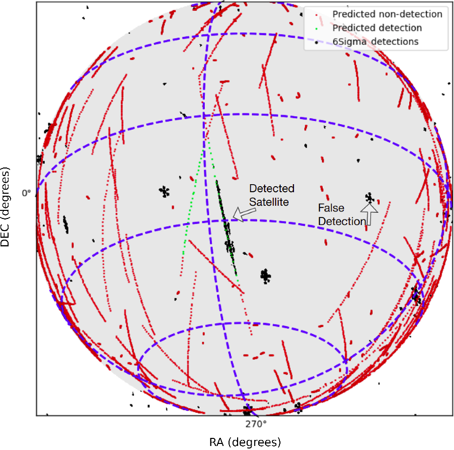
Figure 2. The image shows the visible horizon during one of the 112 s MWA observations. The black markers are detections during this observation. The predicted orbits of all satellites within the visible horizon are plotted in red (or green). If the satellite orbit satisfies all predicted detection criteria (as predicted by Tingay et al. Reference Tingay2013b) and is within MWA’s half power beam, then its trajectory is plotted in green. One of the theoretically detectable satellites being detected by the pipeline is shown and one is not detected. There are several transmitters also detected near the horizon. The figure also shows one of the false detections that takes the shape of the point spread function.
3.3. Parallax analysis
The detections classified as aircraft (Section 4.3) appeared bright enough to be detected outside the MWA’s primary beam, and we estimate the range to these aircraft by performing parallax measurements. The MWA has 128 tiles, and splitting the array into two sub-arrays enables us to perform parallax measurements to some of these bright nearby events that are within the atmosphere.
The MWA compact configuration baselines were sorted in longitude, using the geometric centres of the baselines. Using this sorted list of baselines, the  $1\,000$ east-most baselines were combined to make an eastern aperture (ensemble of points in the UV plane), and the
  $1\,000$ west-most baselines were combined to make a western aperture. The measurement sets for the eastern and western apertures were created by using the splitFootnote g task in Common Astronomy Software Applications (CASAFootnote h) by providing the baseline configuration for both the apertures.
Difference images for the full MWA compact array, eastern aperture, and western aperture were produced for one of the time steps in which an aircraft was present. However, the UV coverages of the three apertures are different, resulting in different beams sizes. Hence, we address the problem by performing CLEAN and using a low-resolution restoring beam corresponding to the lowest resolution of the three apertures. Due to the reflection signal being present in many frequency channels, we enabled the multi-frequency synthesis feature of WSCLEAN while imaging. The centres of the eastern and western apertures were calculated using the geocentric coordinates of the tiles obtained from the measurement set using casa-core.Footnote i The two apertures result in a parallax baseline of  $228.2$ m.
The difference images made using the eastern and western apertures showed the parallax shift in the apparent position of the aircraft, as shown in Figure 3. Using the maximum brightness points and the centres of the two apertures, the LOS range to the aircraft was calculated as in Earl (Reference Earl2015) to be  $20 \pm 2$ km. The aircraft was detected at an azimuth of
  $82.6^\circ$ and an elevation of
  $26.3^\circ$, placing it at an altitude of
  $9 \pm 1$ km (height of most civil aircraft). Note that although the baselines were sorted in longitude to maximise the East-West separation, the centres of the two apertures have a latitude component as well, thus in Figure 3 we see a combination of East-West and North-South offsets in the apparent position.
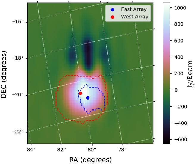
Figure 3.
 $30.72$ MHz bandwidth difference image of an aircraft using the MWA compact array. The blue and the red dotted lines are
  $3 \sigma$ contours of the streak when seen by the eastern and western apertures, respectively. The dots are the corresponding points of maximum brightness. Note that the contour of the eastern aperture image is smaller than that for the western aperture, due to the two sub-arrays having different sensitivities (number of short baselines) towards the aircraft’s altitude.
4. Results
4.1. Satellite candidates
Visual inspection of the detection maps for each of the observations was performed, and the events that plausibly matched in time and position with known objects at multiple time steps were classified as satellite candidate detections. A total of 74 unique LEO objects were detected over multiple passes, of which 15 were upper stage rocket body debris. The LOS ranges for these satellites were obtained for the time steps they were detected (calculated using the two line element (TLE) values). The range values, along with RCS, peak flux densities, and operational statuses for these detected objects, are tabulated in Table 2 (the UTC time, frequency, and angular location of all the detected events for the observations mentioned in Table 2 are available in Prabu et al. Reference Prabu, Hancock, Zhang and Tingay2020a). An example DSNRS plot, illustrating the range of frequencies and times for which a satellite was detected, is shown in Figure 4.
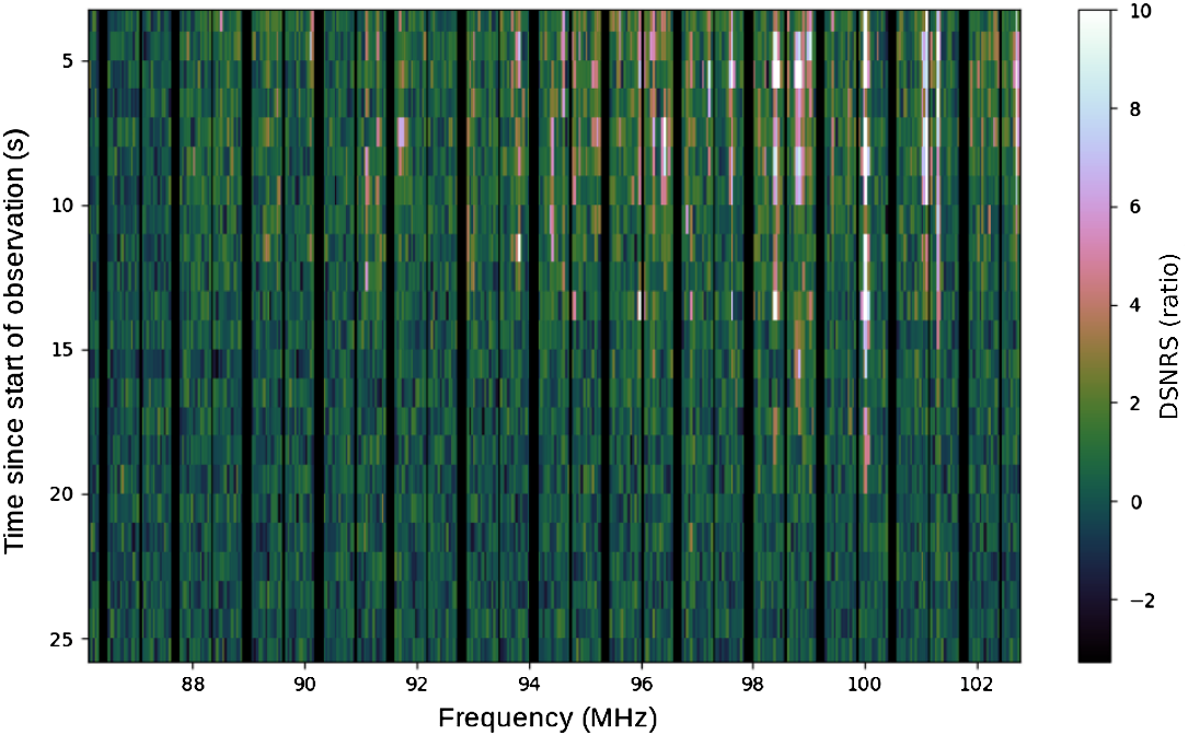
Figure 4. DSNRS plot for ZIYUAN 3 (ZY 3). The plot shows the different FM frequencies reflected by the satellite. The black vertical lines in the figure are due to the flagging of trailing, central, and leading fine frequency channels in every coarse channel.
Two satellites, the CubeSats DUCHIFAT-1 and UKUBE-1, were detected due to out-of-band transmissions in the FM band, rather than reflections (as previously observed by Zhang et al. Reference Zhang2018 and Prabu et al. Reference Prabu, Hancock, Zhang and Tingay2020b).
Table 2. Detected Satellites/Debris and their properties.
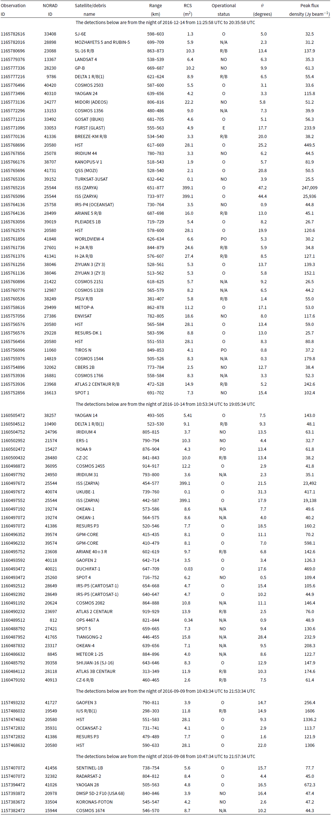
Legend: O=Operational, R/B=Rocket Body, NO=Non-Operational, PO=Partially Operational, N/A=Not Available. The table summarises the properties of all the detected satellites. It provides the satellite’s North American Aerospace Defence (NORAD) ID, the range of distance over which it was detected, its Radar Cross Section (RCS [Obtained from https://celestrak.com/pub/satcat.txt.]), the zenith angle  $(\theta)$, and the primary beam corrected peak flux density as seen in the brightest 40 kHz frequency channel. Note that the operational status (https://celestrak.com/satcat/satcat-format.php.) may not be accurate as the information source does not list the date it was last updated. Note that the Observation ID is the GPS time of the start of the observation.
4.2. Meteor candidates
The observations from one of the nights used in this work (2016 December 14) coincided with the Geminids meteor shower. The pipeline detected many reflections from objects that had angular speeds much greater than expected for LEO objects. These objects moved approximately 10 degrees in a single 2 s time step and are FM reflections from the ionised trails of meteors, as previously observed by Zhang et al. (Reference Zhang2018) with the MWA. An example is shown in Figure 5. These events often appeared much brighter than satellites and were often pointing in the direction of the Geminids radiant.
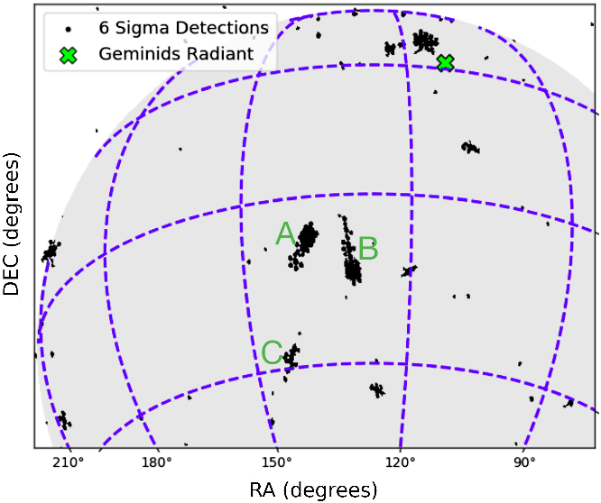
Figure 5. Three of the detected meteors are shown in regions A, B and C. Meteor-A and meteor-C point in the direction of the Geminids Radiant while meteor-B could be a sporadic meteor.
4.3. Aircraft
Nineteen aircraft passes were detected by the pipeline, due to their large reflecting areas and smaller ranges. Most of these aircraft flew North-South over the MWA (a very common flight path for flights between Singapore/Malaysia/northern WA locations and Perth). These reflections appeared very bright (approximately 2800 Jy beam
-1 peak flux density in a  $30.72$ MHz bandwidth difference image), and we utilised parallax to determine their altitudes (Section 3.3).
4.4. Transmitters and unknown objects
Transmitters near the horizon were often detected. These transmitters are not removed through difference images as they are at a fixed azimuth and elevation, hence appear to move in celestial coordinates with time. In future observations, these azimuths/elevations will be masked in order to prevent the pipeline from detecting these transmitters. The transmitters are seen at multiple FM frequencies.
We also detected several events that had angular speeds very similar to LEO objects but did not coincide with any known orbits in the TLE catalog. These are likely to be either satellites with outdated TLEs or uncatalogued objects (intentionally or otherwise). In future, we will investigate these events further by performing orbit determination estimates.
4.5. False positives
The noise in difference images mainly consists of thermal noise and is assumed to follow Gaussian statistics. Due to the large volume of data used in this work, thermal noise fluctuations can trigger the  $6 \sigma$ threshold of the detection pipeline, and hence it is important that we quantify these false positives. However, since we constrain the pipeline to allow only the brightest detection per time step and per frequency channel, the number of false detections is reduced in the presence of a bright reflection event that is seen in multiple frequencies.
In order to investigate the number of false positives, we ran our pipeline again but only on the 380 fine channels outside the FM band (i.e outside 87.5–108 MHz, which is the FM band in Australia). By doing so, we only detect the false positives as the reflection events are confined to the FM band. Note that observations that had no transmitting satellites were used for this analysis, as the transmitted signals from satellites were not confined to the FM band.
We obtained an average of 13 false detections per minute, for the 380 fine frequency channels used. Thus for a full bandwidth observation, and in the absence of any satellite detection, we would obtain approximately 26 false detections per minute. However, since we utilise other tools such as DSNRS (frequency and time analysis) and detection maps (position and time analysis), to investigate these events further, the probability of classifying one of these events as a LEO object is insignificantly small.
5. Discussion
5.1. Detection completeness
Tingay et al. (Reference Tingay2013b) predict that satellites with an RCS greater than  $0.79$
  ${\rm m}^2$ and with an LOS range less than
  $1\,000$ km can be detected using the MWA in the FM band using non-coherent techniques. All the satellites/debris that passed through the MWA’s half power beam with a shortest range during a pass less than
  $2\,000$ km were identified and their RCS, along with the shortest range during pass, are plotted in Figure 6. All of the detected objects in this work (except three CubeSats and one MiniSat) were detected within the theoretically predicted parameter space. Two of the CubeSats (DUCHIFAT-1 and UKUBE-1) were detected due to out-of band transmissions in the FM band (as previously observed by Zhang et al. Reference Zhang2018 and Prabu et al. Reference Prabu, Hancock, Zhang and Tingay2020b) and the other CubeSat and MiniSat were detected through FM reflections. Some satellites such as the ISS and Hubble Space Telescope (HST) were also detected outside the MWA’s primary beam due to their large RCS.

Figure 6. The RCS and the shortest range for all the satellites/debris passes above the horizon within the half power beam and with a range less than 2000 km. Note that although a satellite can appear in two consecutive observation IDs, it appears in the above plot as a single datum e.g. the ISS is detected in four observations according to Table 2, but only appears twice in the above plot (two rightmost points with the largest RCS) because those four observations covered two passes.
From Figure 6 it can be seen that not all the satellites in the predicted parameter space were detected. This could be due to a number of reasons, for example, unfavourable reflection geometries, or our pipeline being constrained to allow only one detection per time step per frequency channel. One significant reason could be that the RCS values are estimated by the US Space Surveillance Network (SSN) (Sridharan Reference Sridharan and Pensa1998) using VHF/UHF/S-Band radars and are very likely to be quite different at the FM frequencies considered in this work. The RCS can also vary drastically as the transmitter-target-MWA reflection geometry changes and as the satellite tumbles. Also, the radar measured RCS is usually for a direct back-scatter/reflection where the transmitter and the receiver are co-located, as opposed to our method where we are looking at an oblique scattering of radiation (bi-static radar). Hence, we use the cataloged RCS values as an order of magnitude guide only. Also, since the classification of an event as a LEO object is done by visual inspection, it is possible that we missed detections near the horizon as it is usually crowded with many orbits due to projection effects as seen in Figure 2.
From Table 2 we can see that many satellites, such as the HST, were detected multiple times on the same night, demonstrating the MWA’s re-acquisition capability for large objects. Many objects such as rocket body debris and non-operational satellites were also detected, and for these objects passive space surveillance is the only way we can track them, thus demonstrating the MWA’s utility to track large obsolete objects. One such example is the object OPS 4467 A (NORAD ID 812). This satellite is the oldest object detected in our work and was launched in 1964.
Other interesting detected objects from Table 2 are MOZHAYETS-5 and RUBIN-5, which were launched together on the same rocket. RUBIN-5 was designed to stay attached to the payload adapter while MOZHAYETS-5 failed to detach from the adapter and hence they appear together as a single object in Table 2.
In one of the observations, the ISS was detected near the horizon with a peak flux density of  $247\,009$ Jy beam-1 in one of the 40 kHz fine frequency channels. This could be due to a favourable reflection geometry and reflections from its very large solar panel arrays.
5.2. RFI environment analysis
There have been many recent studies that investigate the impact of satellite constellations on astronomy at optical, infrared, and radio wavelengths (McDowell Reference McDowell2020; Gallozzi et al. Reference Gallozzi, Scardia and Maris2020; Hainaut & Williams Reference Hainaut and Williams2020). Here, along with demonstrating SDA capabilities with the MWA, we can use our data to examine the impact of the signals we detect on low-frequency radio interferometers such as the MWA, or the future SKA, in the FM band. Rather than useful information on satellites in LEO, out signals can be considered disruptive sources of RFI. Understanding these signals as RFI in the MRO environment is of vital importance, as this is the site where the low-frequency component of the SKA will soon be built.
First we examine the data contained in Table 2 as a function of azimuth and elevation (data are binned in  $0.5^{\circ}$ resolution). In order to determine the maximum impact of the RFI in any given direction, we plot the maximum SNR as a function of azimuth and elevation in the top-left panel of Figure 7. Complex structure across the sky from these sources of RFI is immediately apparent.
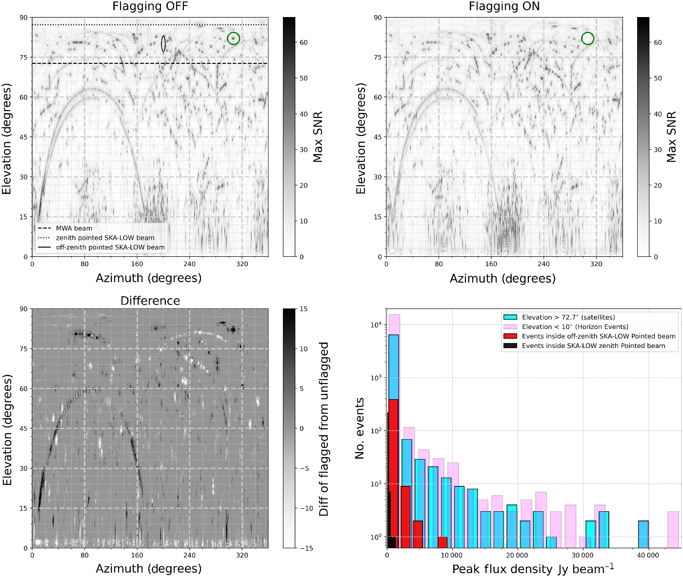
Figure 7. The Flagging OFF panel shows the maximum SNR detected using our pipeline at a given azimuth and elevation, using the data from Table 2. The panel also shows 2 different beam pointings for SKA-LOW station and 1 zenith pointed beam for MWA. The Flagging ON panel shows the events detected by the same pipeline after running AOFLAGGER on the measurement sets, applying the default built-in MWA flagging strategy. The event inside the green circle in the top two panels is an example of an event beging flagged by AOFLAGGER. The bottom-left panel shows the difference of the two top panels (top-right subtracted from top-left), showing the different events detected by AOFLAGGER; black denotes signals detected and removed by AOFLAGGER, white denotes weaker signals revealed by the pipeline after AOFLAGGER has removed strong signals. The bottom-right panel shows the apparent peak intensity distribution for events detected in the different regions shown in the top-left panel and described in the text.
At low elevations ( $<30^{\circ}$), we see periodicity in the strength of RFI detection as a function of azimuth. This reflects the sensitivity of the north-south dipoles (YY polarisation; sensitivity in east-west direction) and the east-west dipoles (XX polarisation; sensitivity in the north-south direction) that form the MWA antennas. Of these four sensitive horizon directions, we observe many high SNR events south of the array, due to the ducting of signals from powerful FM transmitters located in Perth and Geraldton (cities located south of the MWA).
We also note that we do not detect many high SNR events near the zenith (above an elevation of  $85^{\circ}$), perhaps due to inappropriate reflection geometries for the signal from transmitters near the horizon, but also likely due to the fact that the density of satellites in the sky is minimised towards the zenith (due to the projected volume of sky observed increases as we go away from the zenith). As the MWA beam was pointed towards the zenith, we can show the region within the beam as a constant zenith angle limit in Figure 7. For the MWA FOV at zenith, we can see a significant number of high SNR events within the MWA beam.
Similarly, we also indicate a zenith pointed beam for a single SKA-Low station, as well as an arbitrary off-zenith pointing (azimuth= $120^{\circ}$ elevation=
 $80^{\circ}$) for a SKA-Low station (all beams were approximated to be
  $\lambda/d$, where
  $\lambda$ is the wavelength at
  $87.675\,$MHz and d is the diameter of the aperture, i.e.
  $35\,$m for a SKA-Low station and
  $5.65\,$m for an MWA tile). Note that the off-zenith pointed SKA-Low beam appears stretched due to different scales along x and y axes. Here we can see the advantages of a large station size for the SKA, especially when pointed at the zenith. At zenith (and in general), far fewer high SNR events are likely to corrupt SKA data. There are, however, off zenith, still significant numbers of RFI events entering the SKA signal path.
In order to then start to understand how RFI mitigation strategies commonly applied to MWA data perform in terms of identifying these signals and eliminating them from the data, we examined the performance of AOFLAGGER on these signals. AOFLAGGER is the default built-in flagging strategy for MWA data, applied as standard when data are obtained from the MWA archive. As explained earlier, we do not run AOFLAGGER in our pipeline, as we do not want to remove RFI.
We re-ran our full pipeline analysis of all data sets with the addition of the application of AOFLAGGER and repeated the blind detection step on these flagged observations. The results of this analysis are shown in the top-right panel of Figure 7, in direct comparison to the top-left panel, which was obtained without the use of AOFLAGGER. From this comparison, we can see that the difference between the use of AOFLAGGER and not using AOFLAGGER is not massive. Most detected events remain after the use of AOFLAGGER, as they are likely too weak (or diluted). Some differences are highlighted in the comparison.
In order to examine the differences in detail, we plot the difference of the two plots (top-right panel subtracted from the top-left panel in Figure 7). This is shown in the bottom-left panel of Figure 7. The events shown in black are the events that have been detected and flagged by AOFLAGGER. We can see that the track of an aircraft (an inverted U trajectory going North-South in the figure) was detected by AOFLAGGER. But since our blind detection pipeline searches for signals in all fine-frequency channels, we still manage to find the aircraft in some of the fainter channels that were not detected by AOFLAGGER. The aircraft signals are a particularly interesting case to examine, as the signals have a dynamic range that spans strong enough to be detected and flagged by AOFLAGGER, to weak enough to be missed by AOFLAGGER but strong enough to be detected using our pipeline.
There are also some new events detected by the pipeline following the use of AOFLAGGER (shown in white in the difference panel), due to the brightest event being flagged by AOFLAGGER, allowing our pipeline to then detect the next brightest event. As described in Section 3.1, our pipeline is constrained to detect the brightest event in any given time step, at each frequency. After the application of AOFLAGGER, we detected a total of 3 828 additional events, compared to not using AOFLAGGER. This immediately gives us an idea of the impact of our constraint to detect only the brightest events; the additional  $3\,828$ events represent a
  $12.56\%$ increase, showing us that we are likely sacrificing
  $12.56\%$ of events due to the choices made in the pipeline. While not a large effect, future refinements of the pipeline could include the use of AOFLAGGER to recover these events, as well as the use of the DNSRS technique to iteratively perform detection and flagging.
While the use of the maximum detection SNR is useful to indicate the maximum impact of RFI in Figure 7, it is a function of the MWA’s sensitivity. In order to use a measure that can indicate the imapct on other telescopes, such as the SKA, the apparent flux density can be considered. The bottom-right panel of Figure 7 shows the peak intensity distribution for all the events detected: inside the zenith pointed MWA beam (mainly consisting of satellite events); inside the zenith pointed SKA beam; inside the arbitrarily pointed SKA beam; and for events near the horizon ( $<10^{\circ}$). As the figure shows the apparent peak intensity (not primary beam corrected), the true intensity of the events near the horizon are orders of magnitude higher than apparent, as they were detected well outside the primary beam.
With 100 s of events with intensities of 100 s of Jy beam-1 predicted in an arbitrarily pointed SKA-Low beam over the course of a typical observation period, these signals will have to be considered when using the SKA in the FM band (or at any other frequency at which terrestrial transmitters commonly operate). The effect of RFI signals such as these on key science programmes for the SKA (or MWA), such as the Epoch of Reionisation experiment, are complex. Wilensky et al. (Reference Wilensky, Barry, Morales, Hazelton and Byrne2020) considers the threshold for RFI to have a significant effect on the EoR experiment and finds the threshold to be the result of a complex combinations of factors, such as the direction and strength of the RFI, the frequency and time occupancy of the RFI, and the detailed characteristics of the telescope being used.
While such an analysis is beyond the scope of this paper, the information presented here starts to give an indication of the radio astronomy impact of terrestrial transmissions that are reflected off objects in LEO.
6. Conclusions
We have built upon previous work using the MWA as a passive radar system by developing a semi-automated pipeline that searches for reflected signals from LEO satellites in high time and frequency resolution data. Previous detections were performed by manual inspection of full bandwidth difference images, and here we have dramatically increased the number of detections by searching autonomously in every fine frequency channel.
Testing our pipeline on archived MWA data, we detected more than 70 unique LEO objects in 20 h of observation. DUCHIFAT-1 and UKube-1 were detected due to spurious transmissions, while every other detected object was due to FM reflections. The large number of satellite detections through FM reflections alone prove MWA to be a valuable future asset for the global SDA network.
All, except four, of the detected objects were found to lie within the parameter space (range vs RCS) predicted by Tingay et al. (Reference Tingay2013b). However, not all objects that were predicted to be detectable were detected. This could be due to a number of reasons such as tumbling and unfavourable reflection geometries reducing the RCS of the object.
Along with the many satellite detections, we also detected FM reflections from Geminid meteors and aircraft flying over the MWA. Some detected events had angular speeds similar to LEO objects but did not have a satellite orbit match. In the future, we will further examine these unidentified objects by performing orbit determination. We will also use our data to demonstrate a detailed LEO catalog maintenance capability. The Gauss orbit determination technique (Curtis Reference Curtis2013) will be utilised, as we only measure the angular migration of the objects with non-coherent techniques. In future, the detection pipeline used here will be upgraded to preform fully autonomous detections instead of the visual inspection performed here.
We also perform a preliminary analysis of the RFI environment at the Murchison Radio-astronomy Observatory and estimate the impact of signals reflected from objects in LEO, which for astronomers constitute RFI, on the SKA. As part of this analysis, we examined the performance of the MWA’s standard flagging strategy, based on AOFLAGGER, to detect and remove these RFI signals. We found that AOFLAGGER only found 13% of the signals our pipeline found. As such, careful consideration of future RFI flagging strategies for the MWA and the SKA should be given. These results also suggest future refinements for our pipeline.
Many satellites transmit at MWA frequencies for downlink telemetry. Hence, observing in these frequencies could expand our detection window beyond the feasible parameter space (RCS range) shown in this work (observations at these frequencies will have to be performed using a modified form of the pipeline, as we will be detecting objects from LEO-GEO which have different angular speeds, thus requiring different integration times to make difference images). The future detection and characterisation of satellites that unintentionally transmit out of band will also assist in determining the threat of mega-constellations of small satellites to ground-based radio astronomy facilities.
Acknowledgements
This scientific work makes use of the Murchison Radio-astronomy Observatory, operated by CSIRO. The authors acknowledge the Wajarri Yamatji people as the traditional owners of the Observatory site. Support for the operation of the MWA is provided by the Australian Government (NCRIS), under a contract to Curtin University administered by Astronomy Australia Limited. The authors acknowledge the Pawsey Supercomputing Centre which is supported by the Western Australian and Australian Governments. Steve Prabu would like to thank Innovation Central Perth, a collaboration of Cisco, Curtin University, Woodside and CSIRO’s Data61, for their scholarship.
Sofware
We acknowledge the work and the support of the developers of the following Python packages: Astropy (The Astropy Collaboration et al. Curtis 2013; Astropy Collaboration et al. 2018), Numpy (van der Walt, Colbert, & Varoquaux Reference van der Walt, Colbert and Varoquaux2011), Scipy (Jones et al. Reference Jones2001), matplotlib (Hunter Reference Hunter2007), SkyFieldFootnote k and Ephem.Footnote l The work also used WSCLEAN (Offringa et al. Reference Offringa2014; Offringa & Smirnov Reference Offringa and Smirnov2017) for making fits images and DS9Footnote m for visualization purposes.


