Dynamical Stability and Geometrical Diagnostic of the Power Law K-Essence Dark Energy Model with Interaction


1
Department of Physics, Liaoning Normal University, Dalian 116029, China
2
School of Liberal Arts and Sciences, North China Institute of Aerospace Engineering, Langfang 065000, China
3
Peng Huanwu Center for Fundamental Theory, Hefei 230026, China
*
Author to whom correspondence should be addressed.
Universe 2020, 6(12), 244; https://doi.org/10.3390/universe6120244
Submission received: 21 October 2020
/
Revised: 11 December 2020
/
Accepted: 13 December 2020
/
Published: 18 December 2020
(This article belongs to the Special Issue Probing the Dark Universe with Theory and Observations)
Abstract
:We investigate the cosmological evolution of the power law k-essence dark energy (DE) model with interaction in FRWL spacetime with the Lagrangian that contains a kinetic function . Concretely, the cosmological evolution in this model are discussed by the autonomous dynamical system and its critical points, together with the corresponding cosmological quantities, such as , , , and q, are calculated at each critical point. The evolutionary trajectories are drawn in order to show the dynamical process on the phases plan around the critical points. The result that we obtained indicates that there are four dynamical attractors, and all of them correspond to an accelerating expansion of universe for certain potential parameter and coupling parameter. Besides that, the geometrical diagnostic by the statefinder hierarchy and of this scalar field model are numerically obtained by the phase components, as an extended null diagnostic for the cosmological constant. This diagnostic shows that both the potential parameter and interaction parameter play important roles in the evolution of the statefinder hierarchy.
1. Introduction
There are two important stages in cosmology, the early inflation and the late time accelerated expansion. The inflation that we postulate is to explain some issues, such as the flat problem and the horizon problem, etc. While, the accelerating expansion is based on the observations on the luminosity-redshift relation of distant Ia supernovas [1,2], Cosmic Microwave Background [3], and Baryon Acoustic Oscillations [4], which indicate that the current energy density in the universe is composed by 68.3% dark energy (DE), 26.8% dark matter (DM), and 4.9% baryons [5] in order to drive the late time acceleration approximately. More details and cosmic constrain by observation are in [6,7,8,9]. Since its first observation in 1998, over the last twenty years, there have been many models to make explanation for the physical mechanism of this phenomenon. Among them, the simplest one is the CDM model with a constant equation of state (EoS) , which provides the negative pressure for the expansion. CDM model is in good accordance with the observation, but it has some crucial problems, such as the cosmological constant problem, the age problem [10,11,12,13,14], and the tensions on the parameters and in the CDM model in recent years [15,16,17,18,19,20]. Instead of the CDM model, there is a class of phenomenological models with a scalar field to reconcile the problems above; for example, quintessence, phantom, quintom, tachyon, k-essence, and DBI models, etc. Among them, the quintessence model is one of the most popular one [21]. Its Lagrangian density , being the pressure, in the action is described by a single scalar field , and a canonical kinetic energy . To some extent, the quintessence model can describe a range of EoS necessary for an accelerated expansion, but the single-field quintessence with a canonical kinetic term limits the EoS w to be less than . To this point, the quintom model with multiple fields [22] and some k-essence models with non-canonical kinetic terms are developed in order to realize the crossing of the phantom divide. Additionally, the combination of data sets Plank+R16+JLA support this point, such as in [15], for .
It is known that the k-essence model is a better substitution for the quintessence model. Although it firstly originated from k-inflation coming from the string theory to explain the early inflation of the universe [23]; fortunately, it could also explain the late time accelerated expansion as DE [24], even in the form as a decent generalization of many scalar field dark energy models. Unlike the canonical kinetics that are defined by the quintessence model, the k-essence model provides a variety of non-canonical terms, i.e., [25], which contains higher order terms of X. As a result, the k-essence model with non-canonical kinetic term in Largragian can also reconcile the tension problem by making the EoS smaller than . The form of was first discussed as a purely kinetic function , with a constant potential, [26]. Further more, two common forms along with potential are and , which were widely investigated in [27,28]. Some of the modified kinetic terms were discussed, such as [29], [30], and [31] etc., which belongs to the class of power law k-essence dark energy model with the power law function . The approximation of the potential in scalar field dark energy models are discussed in [32], with both canonical and noncanonical kinetic terms.
In another aspect, from the matter clustering properties, dark matter (DM) and dark energy are not the same substance; however, there are researches regarding the interactions between them, even some nonlinear interaction forms [33,34,35,36,37], which can provide a mechanism for generating acceleration. By the recent observation, the interaction between DM and DE is too little to alleviate the coincidence problem, while, in our work, the k-essence model with the interaction between DM and DE can be a candidate, which helps to explain the tension and tension between CMB and structure formation measurements [15,16,17].
The aim of this paper, which is based on the researches above, is to consider a model with , where , , and [38], together with a certain kind of interaction Q. We investigate the possible cosmological behavior of this model in Friedmann–Robertson–Walker–Lemaître (FRWL) spacetime by performing a phase-space and stability analysis. The theory are based on [39,40] judging the stability of the critical points by the eigenvalues; whereas, in this model for the convenience of calculation, it prefers the method by the determinant and trace of the Jacobian matrix of the autonomous differential equations [41]. Some cosmological quantities will be calculated for each critical point, such as the dark energy density parameter , the equation of state (EoS) parameter of dark energy, the sound speed , and the deceleration parameter q.
Finally, in order to distinguish this k-essence model from CDM model, there are two main kinds of “null measure”: the Om diagnostic and the statefinder diagnostic. Om is constructed from the Hubble parameter H, and it provides a null test of the CDM model [42,43]. In recent years, in order to distinguish those models from the best fitting model, the CDM model, the statefinder hierarchy is used, which originate from statefinder diagnostic [44,45]. The statefinder pair , is composed by the scale factor with its second and third derivatives; however, the statefinder hierarchy is based on the even higher derivatives [46]. In this paper, statefinder hierarchy and are analyzed to the scalar dark energy model by the phase components (the auxiliary variables) in the autonomous equations, unlike the method that was mentioned before, which depends on the cosmological quantities. It shows that the hierarchies are varied from two parameters and by the trajectories. This novel method is based on [47,48,49], which is used for the quintessence model and model, and it could be generated to a range of scalar DE models in the future.
This paper is organized, as follows: in the following section, we review k-essence dark energy models and its stability analysis. In the third section, we consider the dynamics of the k-essence scalar field with the interaction (the coupling parameter is a real arbitrary constant). In the fourth section, the statefinder diagnostic and statefinder hierarchy are analyzed in order to distinguish from CDM model. Finally, we close with a few concluding remarks in the fifth section.
2. The Power Law K-Essence Dark Energy Model and Its Stability Analysis
We consider k-essence dark energy models with Lagrangian
where the kinetic term and potential term are analytic functions of X and , respectively. Throughout this paper, we will work with a flat, homogeneous, and isotropic FRWL spacetime having signature and in units . We are interested in the power law k-essence with a general form of kinetic term , which has been studied in [29,38,50]. Hence, the scalar field is redefined as the one in [29]. Consequently, Equation (1) is rewritten as ), where the new kenetic term and new potential term . Subsequently, the corresponding energy density , the EoS parameter and the effective sound speed are, respectively, given by
where and . The sound speed comes from the equation describing the evolution of linear adiabatic perturbations in a k-essence dominated universe [29,51] (a non-adiabatic perturbation of k-essence has been discussed in [52,53], here we only consider the case of adiabatic perturbation). From Equations (3) and (4), it has . Meanwhile, by considering the stability of solutions with respect to inhomogeneous perturbations as , it constrains the range . It follows that the k-essence model in this paper does not permit phantom behaviour.
In the following discussion, we neglect baryonic matter and the radiation in the matter component. Subsequently, the Friedmann equations take the form
where is the Hubble parameter, and are the DE and DM density, respectively. The equation of motion for the k-essence field is given by
where . Equations (5) and (6) are usually transformed into an autonomous dynamical system when performing the phase-space and stability analysis. Being derived from the Friedmann eqs., we obtain , which implies a continuous eq. . Because, in this model, the density is composed by two parts, the dark energy density and the matter density, i.e., , with the interaction Q between DM and DE, and do not separately satisfy conservation laws. Subsequently, the following two equations are conceived as:
Here, . For , there is a transfer of energy from dark energy to dark matter. The case of , as in no interaction, was discussed in the former paper [38]. While, in this paper, the interaction is chosen by , which means that the transformation between dark energy and dark matter happen, to some degree, in that circumstance. By Equations (8) and (9), to keep the physical dimensionality, we have to set as a dimensionless parameter [33].
By setting the phase components, the auxiliary variables are defined as
in order to transform the cosmological Equations (5) and (6) into an autonomous dynamical system , by considering (8) and (9), where the prime is the derivative with respect to . Subsequently, after solving the eqs. , the critical points = are obtained. To discuss the stability of each critical point, we expand = around the critical points = by setting with the perturbational variables (see, for example, Refs. [41,54,55,56,57,58]). Up to the first order we acquire with the matrix determined by
The matrix contains the coefficients of the perturbation equations, and thus its eigenvalues determine the stability of the critical points. In this 2-dim system, which has two eigenvalues of M, for hyperbolic critical points, all of the eigenvalues have real parts that are different from zero: sink for the negative real parts is stable, saddle for real parts of different sign is unstable, and source for positive real parts is unstable. However, for the convenience of calculation in this model, an alternative way to judge the stability of the critical points in a 2-dim system is given by the trace tr and determinant .
For the more general linear interaction form , the autonomous dynamical equations are derived, as follows:
for ; while, for , the equations turn out to be
where , by assuming in this paper. Because it is hard to obtain an analytic solution as a critical point from the equations above with three parameters , , and , it has to be simplified by two cases in the next step, i.e., and , respectively. However, we only analyze in this paper due to the unsatisfactory for . Besides that, the values of and are constrained in certain ranges, which are imposed for the observations [18,19,20].
3. The Analysis of Stability for This Dark Energy Model with Interaction
While, when , we have
Additionally, there are other three solutions as the critical points, as follows:
The corresponding density parameter, the EoS, the sound speed, and the deceleration parameter are reexpressed as, respectively,
Equations (16), (17), (21) and (22) form the self-autonomous dynamical systems, which are valid in the whole phase-space, not only at the critical points. The critical points of the autonomous system are obtained by setting the left-hand sides of the equations to zero, namely by solving . Six critical points are obtained, as shown in Table 1, in which we also present the necessary conditions for their existences and stabilities, as well as the corresponding cosmological quantities, , , , and q. With these cosmological quantities, we can investigate the final state of the universe and discuss whether there exists acceleration expansion or not. Physically, it requires , so the auxiliary variables x and y are constrained as . In order to comply with the accelerated expansion, it requires . When considering the sound speed, it has to be . For the existence, it means , and or for each case. The stability means and tr, instead of the analysis by each eigenvalue.
For the power law k-essence dark energy presented in this paper, the specific expression of the , , and tr are as follows:
for the case of ; and,
for the case of .
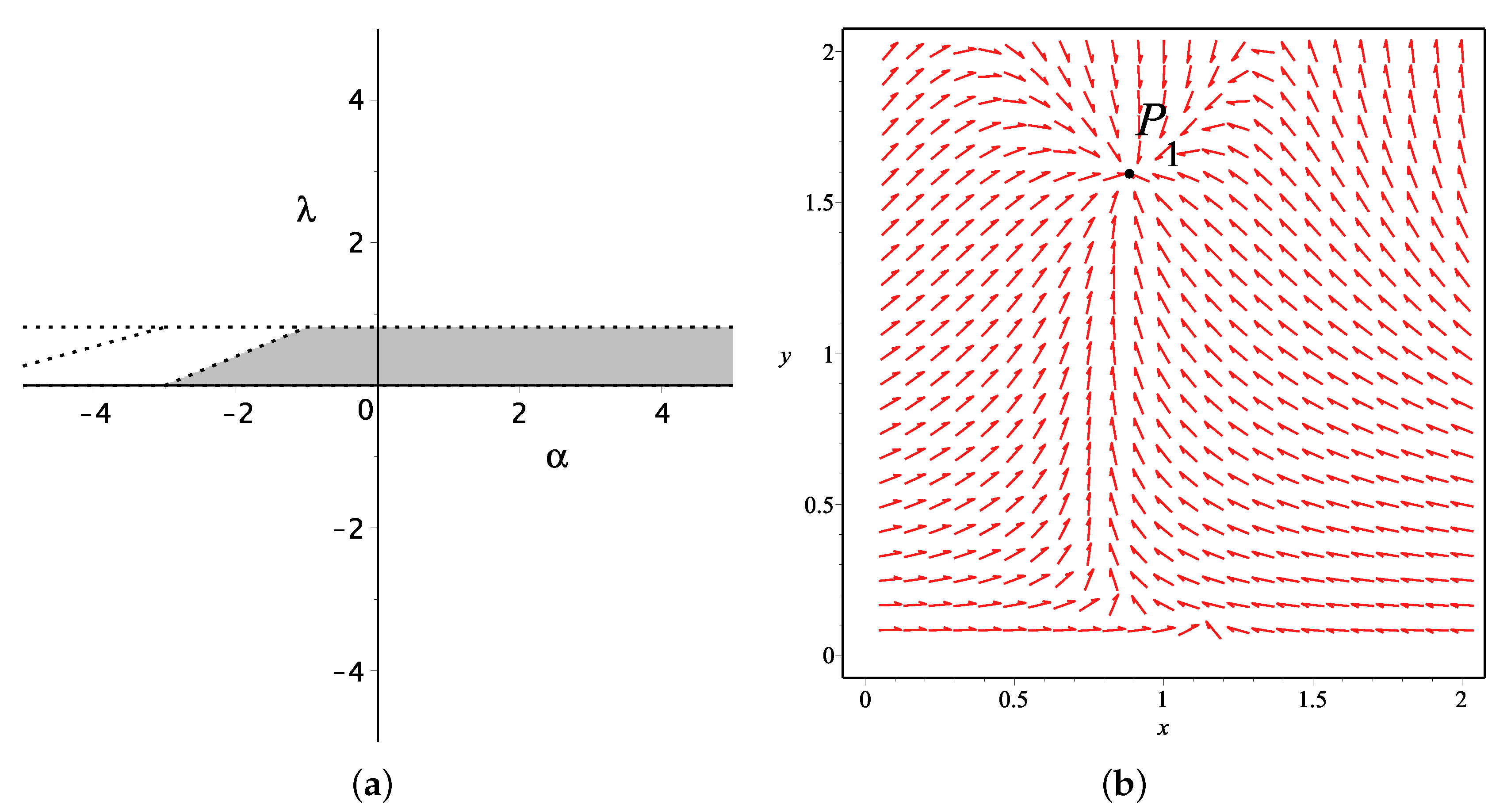
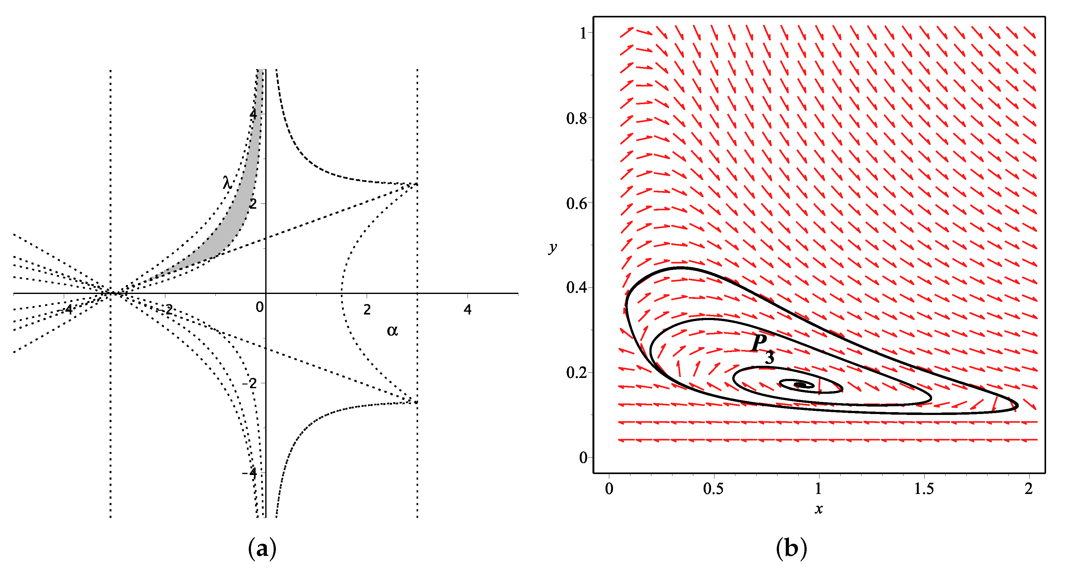
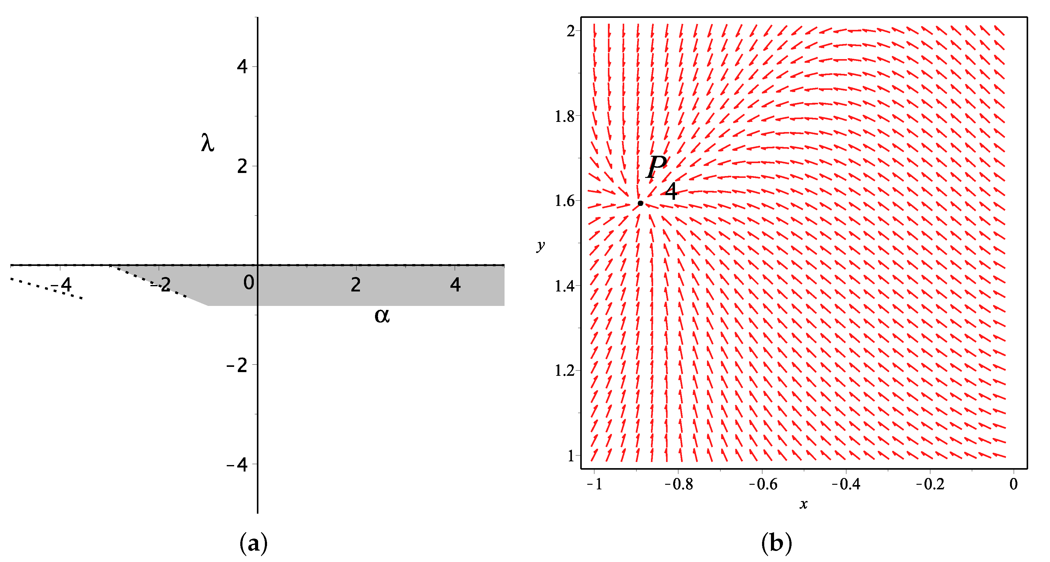
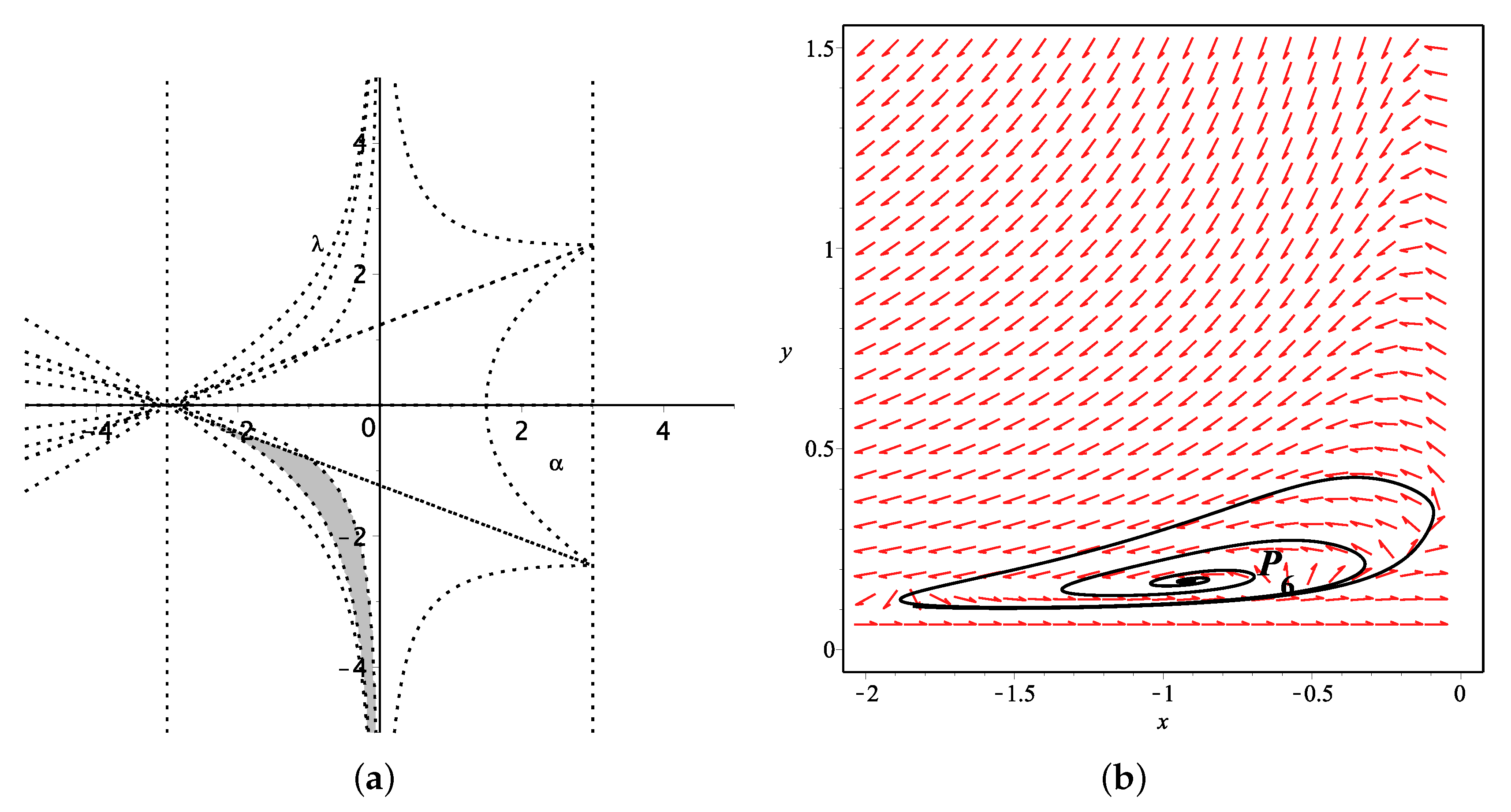
According to the stability conditions of critical points by the determinant and trace, together with those cosmological quantities, we obtain the value range of and in the parameter plane, which makes the critical points stable and causes accelerated expansion, as shown in Table 1. At first, and are excluded by using existence condition. Based on the range of parameters presented in Figure 1a, we plot the stable point and its evolutionary trajectory for and in Figure 1b, as well as , , and (see Figure 2, Figure 3 and Figure 4) with some certain pairs of parameters and , respectively, in order to have a visual understanding of the evolutionary behavior near critical points. Especially, and are spiral attractors, which have spiral evolutionary trajectories around them. Additionally, the evolutionary trajectories of the cosmological quantities are shown in Figure 5 and Figure 6. Below, we will analyze these stable points , , , and one-by-one.
For , it has ; the universe will be dominated by k-essence dark energy. If , then the k-essence would behave like a cosmological constant. The deceleration parameter . The final state of the universe depends on the potential parameter , i.e., the universe expansion would speed up if , it would expand at constant-speed if , and the universe expansion would slow down if .
For , , the universe will be dominated by both k-essence dark energy and dark matter. When and satisfy , lying on the top edge of the grey region in Figure 2a, the k-essence will behave like a cosmological constant. The evolutionary trajectory in the phase space shown in Figure 2b will be spiral around , finally converging to the attractor . The deceleration parameter . The final state of the universe depends on the coupling parameter , i.e., the expansion of the universe will speed up if , will expand in a constant speed if , and will slow down if , respectively.
For , the results are quite like the three critical points that are investigated above. Among the three critical points, and are attractors for some and , as displayed in Figure 3 and Figure 4. Those two points are also physically meaningful; while, does not.
For , it has , the universe will be dominated by k-essence dark energy. If , the k-essence will behave like a cosmological constant. The deceleration parameter , which indicates that the final state of the universe depends on the potential, i.e., the universe expansion will speed up if , will expand with constant-speed if , and it will slow down if .
For , , the universe will be dominated by both k-essence and dark matter. When and satisfy , the k-essence will behave like a cosmological constant. In the phase space, the evolutionary trajectory will be spiral around , and then finally converge to the attractor point. The deceleration parameter , which indicates that the final state of the universe depends on the dark matter: the universe will speed up if , will expand with constant-speed if , and it will slow down if .
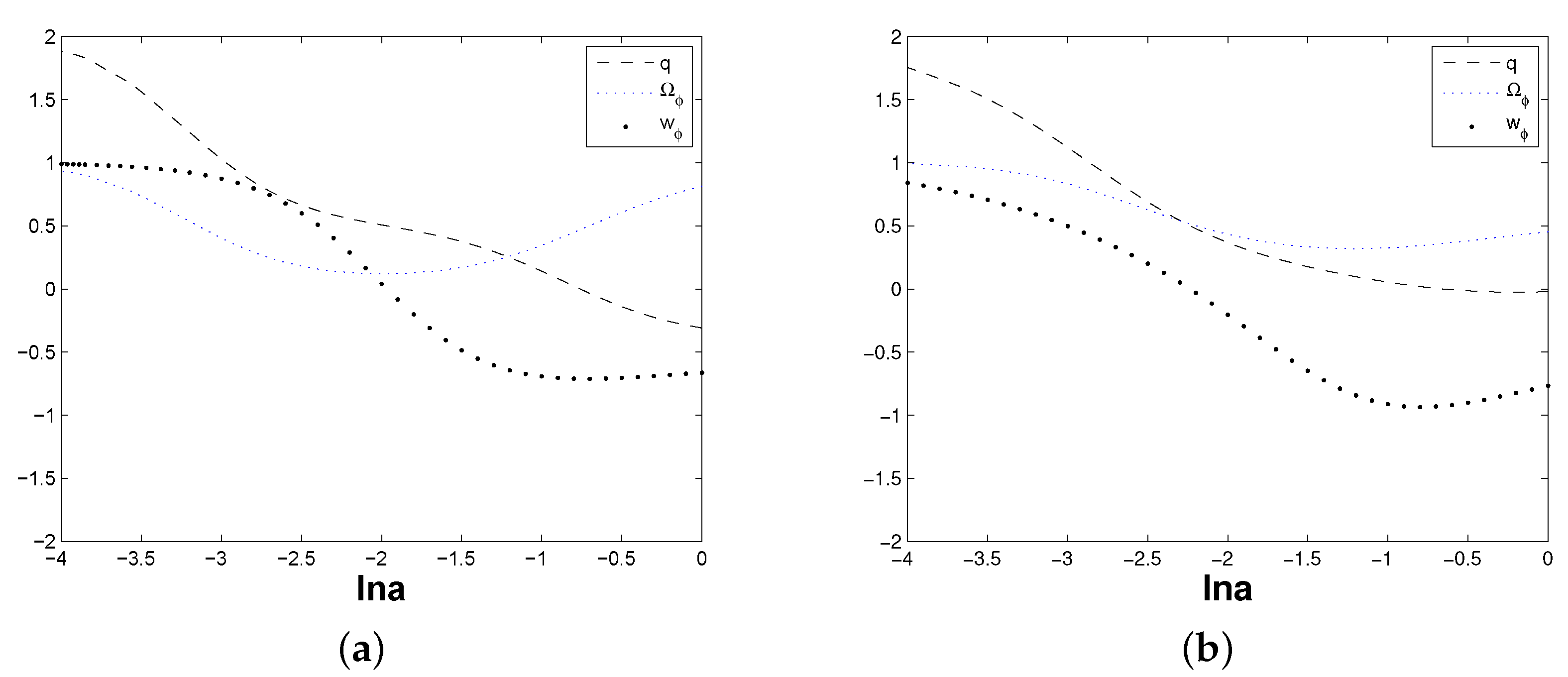
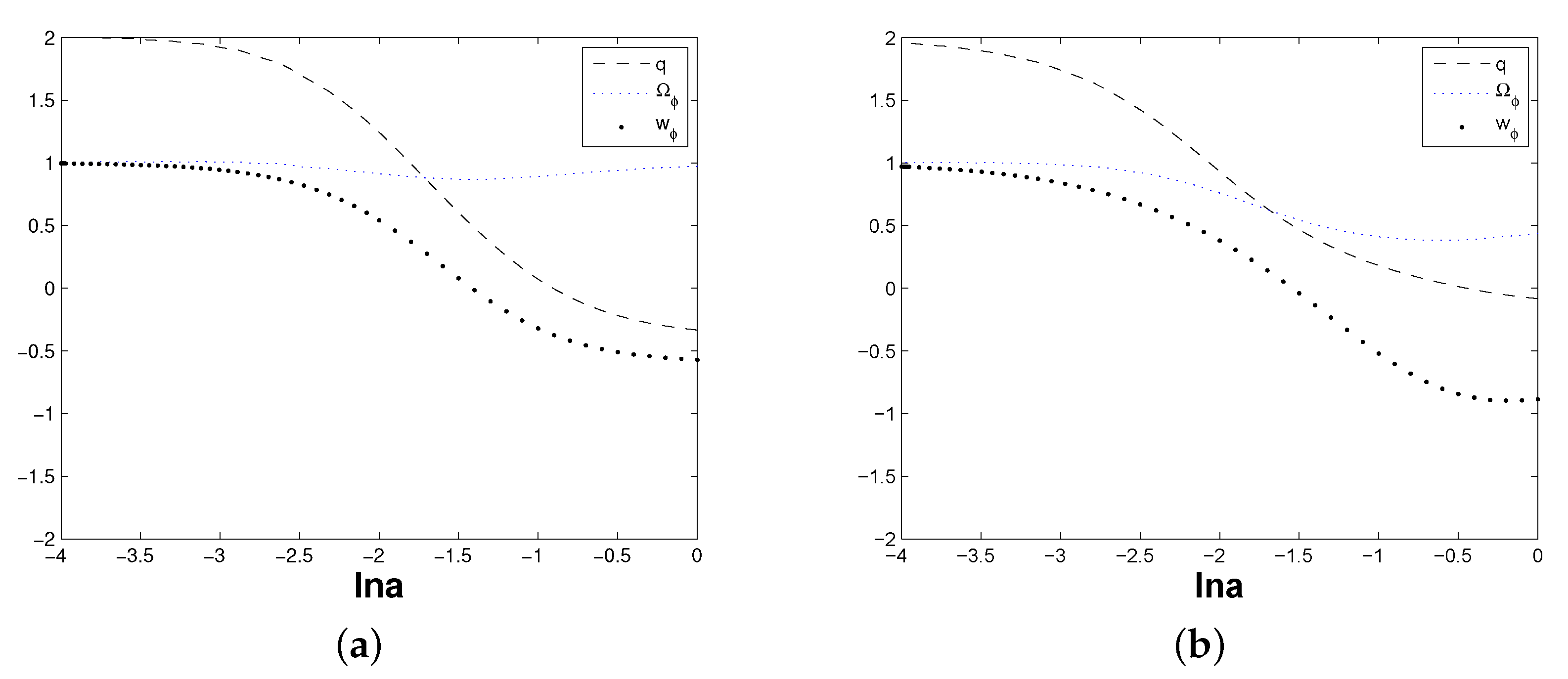
From Figure 5 and Figure 6, it is not difficult to see that the density parameter of DE continuously varies, which indicates that there is the exchange of energy between dark energy and dark matter by the interaction Q, and, at present, the universe is composed by both DE and DM. Meanwhile, the deceleration parameter q evolves from positive to negative values, which shows that the universe experiences a decelerating expansion in the past, and then transforms to an accelerating expansion at present, and keeps on speeding up into the future. Especially, in Figure 5b and Figure 6b, the happens in the early time, which means that, in early time, the dark energy performs in a relativistic matter, which provides positive pressure, and acts as the attraction force to enhance the structure formation. All four evolutional figures show the in the late time universe, which indicates that this k-essence DE model could explain the accelerating expansion of the universe.
4. The Geometric Diagnostic of Statefinder Hierarchy
Because the CDM model is the best fitting for observations until now, the statefinder pair is a way for distinguishing a certain model from the CDM model, by showing the “distance” of trajectories in the plane from the spatially flat CDM model scenario which is a fixed point . Beyond the Hubble parameter and the deceleration parameter , the third order derivative , together with a combination of r and q, which is , become the cosmological diagnostic pair . In terms of and w, the statefinder pair has the following form:
Further, the statefinder hierarchy is an extension of the statefinder pair, which comes from the view point of higher derivatives of the expansion factor , in Taylor expanded: , where , , and . By using , the series and are constructed, as follows. In a spatially flat universe with pressureless matter and a cosmological constant, such as model, could be expressed by parameter q or , where , as follows:
Then the statefinder hierarchy is defined as
Finally, it derived the null diagnostic for the model, the , as follows:
For the model, it always has and . In this paper, we focus on how parameters and effect the statefinder hierarchy and for the k-essence model with coupling . We can obtain the following expressions with interaction Q:
The former methods for analyzing the statefinder pair or the statefinder hierarchy are mainly around purely kinetic k-essence dark energy models, by finding the relations among , and . For the potential, in this paper, it is not as a constant as in PKK and the analytic relation cannot be derived directly; instead, the statefinder hierarchy should be represented by phase components . Along with the numerical method presented in [49], after substituting (16) and (17) into (49) and (50) for , and (21) and (22) into (49) and (50) for , respectively, the statefinder hierarchy and could be expressed by variables x, y with parameters , . We choose the initial points around the attractors separately, and then adjust with a constant , whereas adjust with a constant , in order to see the effect on statefinder hierarchy for each by the figures.
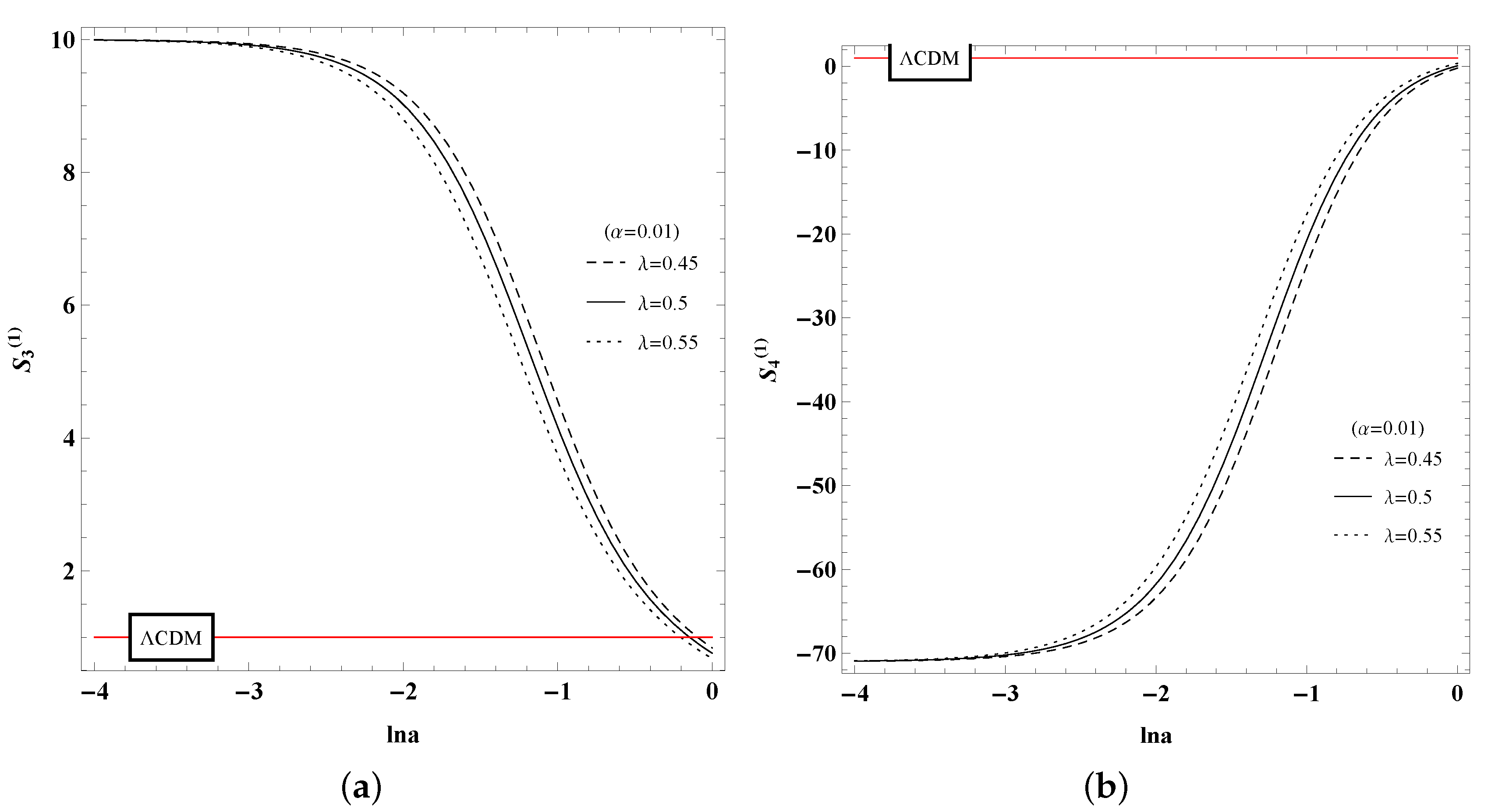
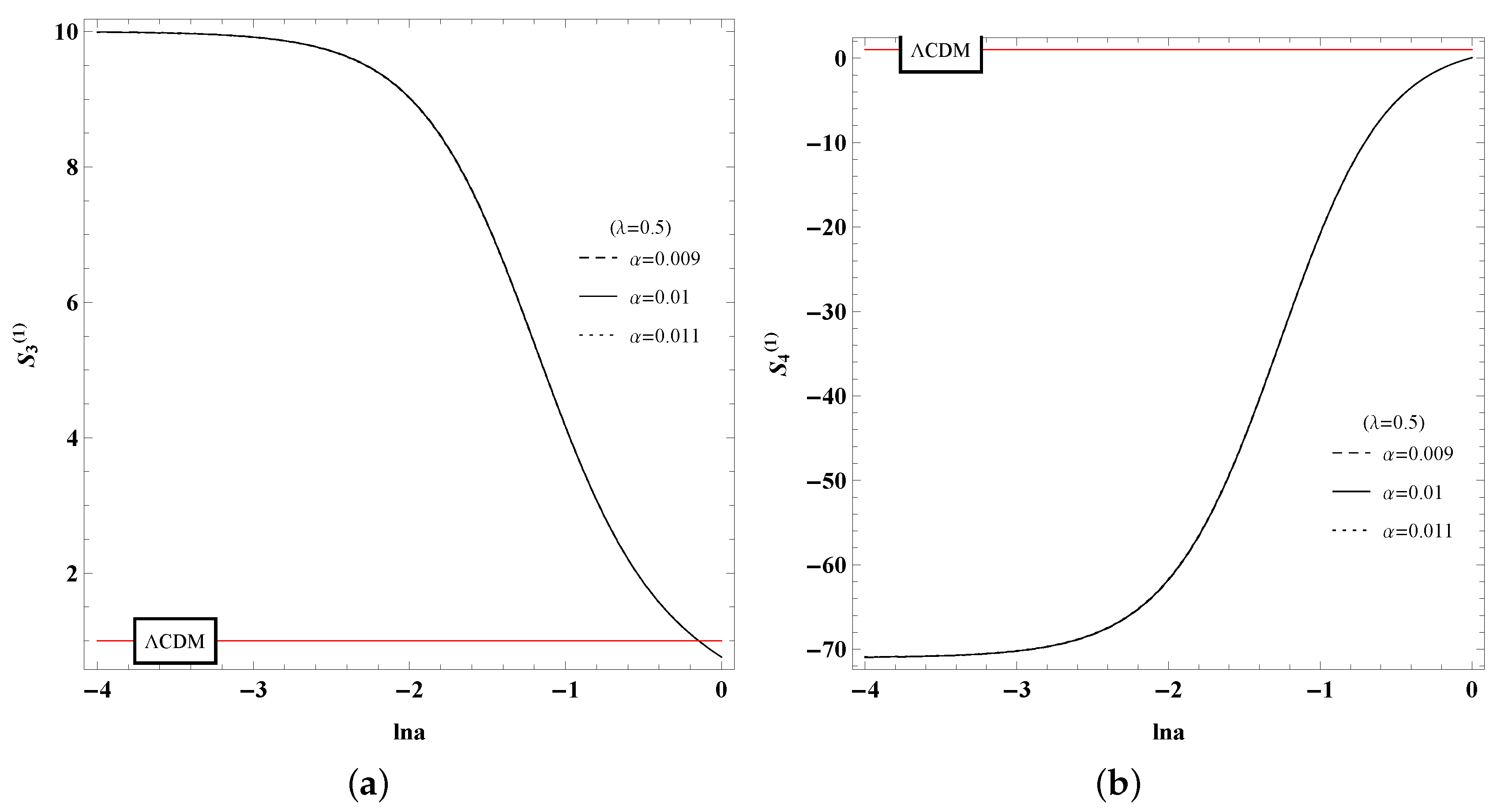
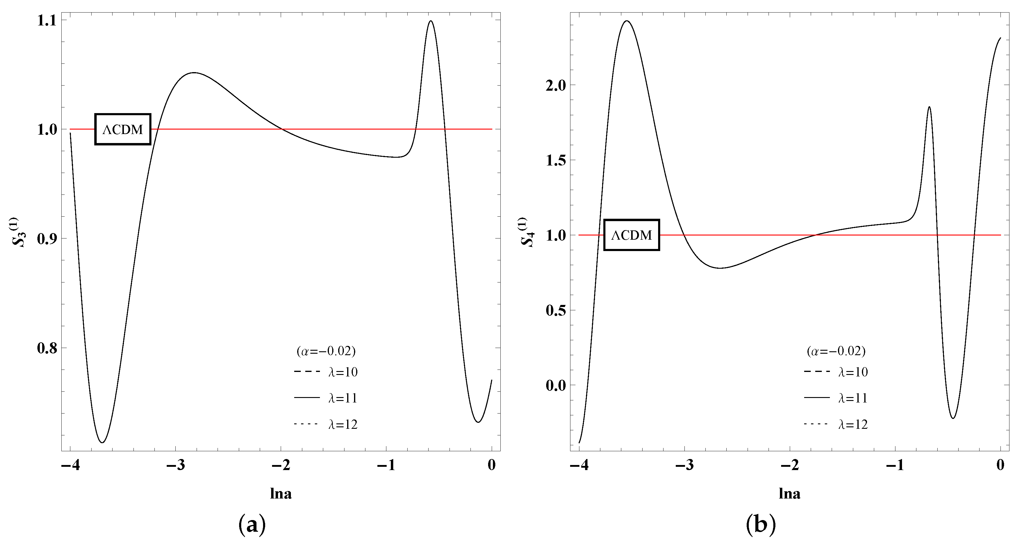
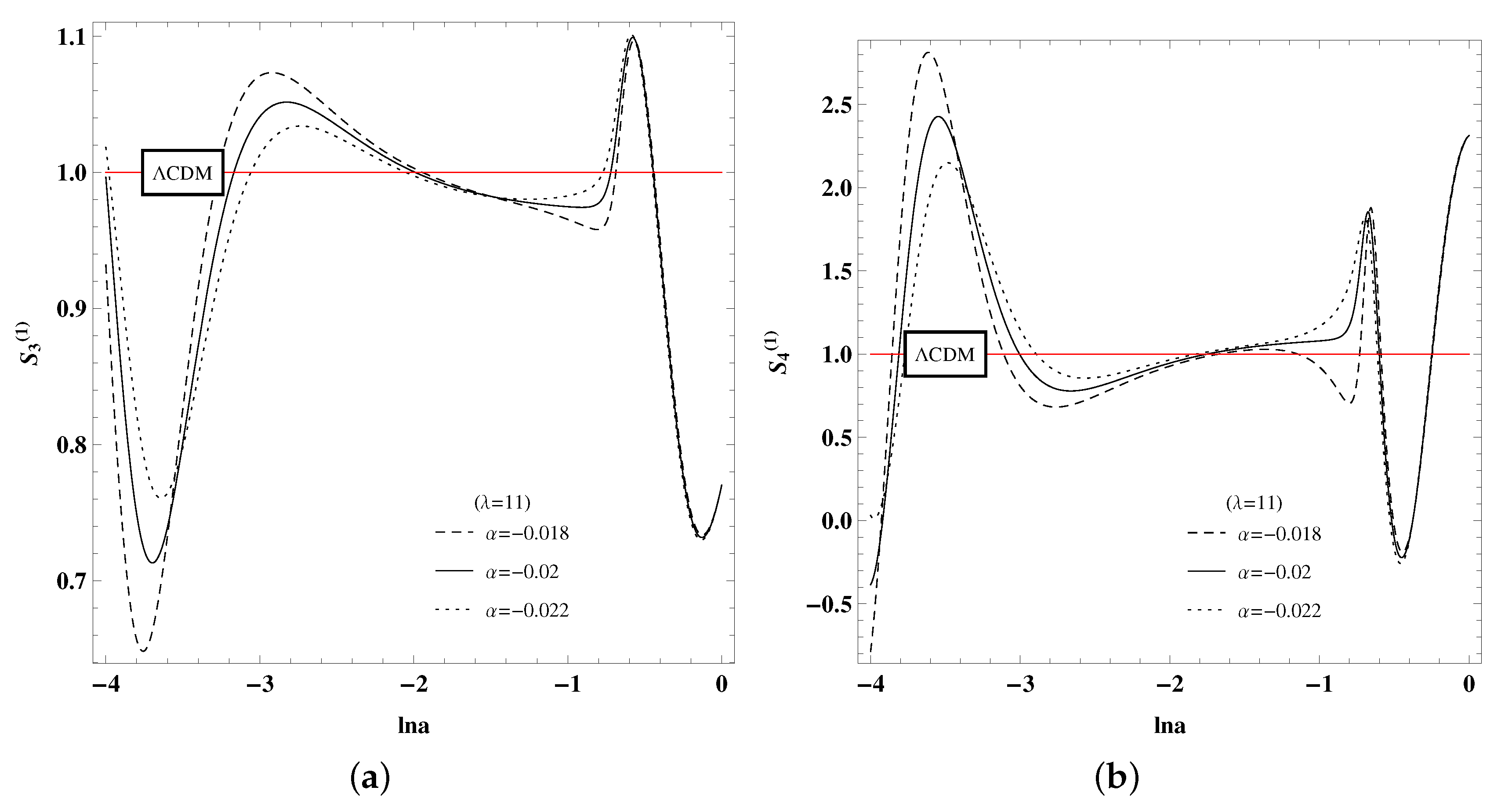
For , from Figure 7, by changing the value of potential parameter with a fixed coupling parameter , the difference of both and evolutionary curves are obvious. However, in Figure 8, there is nearly no difference in both and cases, with the same value of , but different values of . It means that the statefinder hierarchy and are more sensible to the potential parameter than around .
Oppositely, for , there is no difference by changing the potential parameter under the same value for both and in Figure 9, while the statefinder hierarchy shows the sensibility to the coupling parameter under the same value of in Figure 10. That is to say, curves with same value of perform alike, while makes little effect around .
For the case of , i.e., and , the evolutionary curves of the statefinder hierarchy and are analogous to the and , respectively. For all of cases above, the statefinder hierarchy and of the k-essence DE model in this paper can tell the difference from the CDM model, which is a straight line in the figures.
5. Conclusions
In summary, we have deeply investigated the cosmological evolution, the dynamical stability, as well as the geometrical diagnostic of the power law k-essence dark energy model with the Lagrangian containing a kinetic function and interaction in FRWL space time. Concretely, we have not only discussed the influences of the coupling parameter and potential parameter on the evolution of several cosmological quantities (such as the density parameter , EoS of dark energy , the effective sound speed , and deceleration parameter q), but also numerically analyzed the dynamical stability and showed that there are the four dynamical attractors in the phase space. In addition, the statefinder hierarchy and of this dark energy model have been numerically obtained, which shows that the potential parameter has more influence on the evolutions of and than one of the coupling parameter around and ; while, for and , parameter plays a more important role in and .
Author Contributions
B.-H.C.: search the references, plot the figures, write the manuscript; Y.-B.W.: corresponding author, review the manuscript, revise the manuscript; D.-F.X.: plot the figures, arrange the references, edit the manuscript; W.D.: plot the figures, explain the data, search the references; N.Z.: design the research plan, plot the figures, explain the data. All authors have read and agreed to the published version of the manuscript.
Funding
This research was funded by the National Natural Science Foundation of China grant number 12075109, 11575075, 11705079 and 11865012.
Acknowledgments
Y. Wu has been supported by the National Natural Science Foundation of China under grants No.12075109 and No.11575075. W. Yang has been supported by the National Natural Science Foundation of China under grant No.11705079. J. Lu has been supported by the National Natural Science Foundation of China under grants No.11865012.
Conflicts of Interest
There is no conflict of interest.
References
- Riess, A.G.; Filippenko, A.V.; Challis, P.; Clocchiatti, A.; Diercks, A.; Garnavich, P.M.; Gilliland, R.L.; Hogan, C.J.; Jha, S.; Kirshner, R.P.; et al. Observational Evidence from Supernovae for an Accelerating Universe and a Cosmological Constant. Astron. J. 1998, 116, 1009. [Google Scholar] [CrossRef] [Green Version]
- Perlmutter, S.; Aldering, G.; Goldhaber, G.; Knop, R.A.; Nugent, P.; Castro, P.G.; Deustua, S.; Fabbro, S.; Goobar, A.; Groom, D.E.; et al. [The Supernova Cosmology Project] Measurements of Ω and Λ from 42 High-Redshift Supernovae. Astrophys. J. 1999, 517, 565. [Google Scholar] [CrossRef]
- Spergel, D.N.; Verde, L.; Peiris, H.V.; Komatsu, E.; Nolta, M.R.; Bennett, C.L.; Halpern, M.; Hinshaw, G.; Jarosik, N.; Kogut, A.; et al. First-year Wilkinson Microwave Anisotropy Probe (WMAP)* observations: Determination of cosmological parameters. Astrophys. J. Suppl. 2003, 148, 175. [Google Scholar] [CrossRef] [Green Version]
- Eisenstein, D.J.; Zehavi, I.; Hogg, D.W.; Scoccimarro, R.; Blanton, M.R.; Nichol, R.C.; Scranton, R.; Seo, H.J.; Tegmark, M.; Zheng, Z.; et al. Detection of the baryon acoustic peak in the large-scale correlation function of SDSS luminous red galaxies. Astrophys. J. 2005, 633, 560. [Google Scholar] [CrossRef]
- Aghanim, N.; Akrami, Y.; Ashdown, M.; Aumont, J.; Baccigalupi, C.; Ballardini, M.; Banday, A.J.; Barreiro, R.B.; Bartolo, N.; Basak, S.; et al. [Planck Collaboration] Planck 2018 results. VI. Cosmological parameters. Astron. Astrophys. J. 2020, 641, 1–67. [Google Scholar]
- Xu, L.X.; Lu, J.B.; Wang, Y.T. Revisiting generalized Chaplygin gas as a unified dark matter and dark energy model. Eur. Phys. J. C 2012, 72, 1883. [Google Scholar] [CrossRef]
- Xu, L.X.; Wang, Y.T.; Noh, H. Modified Chaplygin gas as a unified dark matter and dark energy model and cosmic constraints. Eur. Phys. J. C 2012, 72, 1931. [Google Scholar] [CrossRef]
- Yang, W.Q.; Li, H.; Wu, Y.B.; Lu, J.B. Cosmological implications of the dark matter equation of state. Int. J. Mod. Phys. D 2017, 26, 1750013. [Google Scholar] [CrossRef]
- Du, M.H.; Yang, W.Q.; Xu, L.X.; Pan, S.; Mota, D.F. Future constraints on dynamical dark-energy using gravitational-wave standard sirens. Phys. Rev. D 2019, 100, 043535. [Google Scholar] [CrossRef] [Green Version]
- Sahni, V.; Starobinsky, A.A. The case for a positive cosmological Λ-term. Int. J. Mod. Phys. D 2000, 9, 373. [Google Scholar] [CrossRef]
- Carroll, S.M. The cosmological constant. Living Rev. Rel. 2001, 4, 1. [Google Scholar] [CrossRef] [PubMed] [Green Version]
- Carroll, S.M.; Hoffman, M.; Trodden, M. Can the dark energy equation-of-state parameter w be less than −1? Phys. Rev. D 2003, 68, 023509. [Google Scholar] [CrossRef] [Green Version]
- Li, M.; Li, X.D.; Wang, S.; Wang, Y. Commun. Dark Energy. Theor. Phys. 2011, 56, 525–604. [Google Scholar]
- Yang, R.J.; Zhang, S.N. The age problem in the ΛCDM model. Mon. Not. R. Astron. Soc. 2010, 407, 1835–1841. [Google Scholar] [CrossRef] [Green Version]
- Valentino, E.D.; Melchiorri, A.; Silk, J. Reconciling Planck with the local value of H0 in extended parameter space. Phys. Lett. B 2016, 761, 242. [Google Scholar] [CrossRef]
- Huang, Q.G.; Wang, K. How the dark energy can reconcile Planck with local determination of the Hubble constant. Eur. Phys. J. C 2016, 76, 506. [Google Scholar] [CrossRef] [Green Version]
- Vagnozzi, S. New physics in light of the H0 tension: An alternative view. Phys. Rev. D 2020, 102, 023518. [Google Scholar] [CrossRef]
- Kumar, S.; Nunes, R.C. Probing the interaction between dark matter and dark energy in the presence of massive neutrinos. Phys. Rev. D 2016, 94, 123511. [Google Scholar] [CrossRef] [Green Version]
- Pan, S.; Yang, W.Q.; Singha, C.; Saridakis, E.N. Observational constraints on sign-changeable interaction models and alleviation of the H0 tension. Phys. Rev. D 2019, 100, 083539. [Google Scholar] [CrossRef] [Green Version]
- Pan, S.; Yang, W.Q.; Valentino, E.D.; Saridakis, E.N.; Chakraborty, S. Interacting scenarios with dynamical dark energy: Observational constraints and alleviation of the H0 tension. Phys. Rev. D 2019, 100, 103520. [Google Scholar] [CrossRef] [Green Version]
- Tsujikawa, S. Quintessence: A Review. Class. Quant. Grav. 2013, 30, 214003. [Google Scholar] [CrossRef] [Green Version]
- Feng, B.; Wang, X.L.; Zhang, X.M. Dark Energy Constraints from the Cosmic Age and Supernova. Phys. Lett. B 2005, 607, 35–41. [Google Scholar] [CrossRef]
- Armendariz-Picon, C.; Damour, T.; Mukhanov, V. K-inflation. Phys. Lett. B 1999, 458, 209–218. [Google Scholar] [CrossRef] [Green Version]
- Armendariz-Picon, C.; Mukhanov, V.; Steinhardt, P.J. A Dynamical Solution to the Problem of a Small Cosmological Constant and Late-time Cosmic Acceleration. Phys. Rev. Lett. 2000, 85, 4438–4441. [Google Scholar] [CrossRef] [Green Version]
- Rendall, A.D. Dynamics of k-essence. Class. Quant. Grav. 2006, 23, 1557–1570. [Google Scholar] [CrossRef] [Green Version]
- Scherrer, R.J. Purely kinetic k-essence as unified dark matter. Phys. Rev. Lett. 2004, 93, 011301. [Google Scholar] [CrossRef] [Green Version]
- Bose, N.; Majumdar, A.S. A k-essence Model of Inflation, Dark Matter and Dark Energy. Phys. Rev. D 2009, 79, 103517. [Google Scholar] [CrossRef] [Green Version]
- Bose, N.; Majumdar, A.S. Unified Model of k-Inflation, Dark Matter and Dark Energy. Phys. Rev. D 2009, 80, 103508. [Google Scholar] [CrossRef] [Green Version]
- Chiba, T.; Okabe, T.; Yamaguchi, M. Kinetically Driven Quintessence. Phys. Rev. D 2000, 62, 023511. [Google Scholar] [CrossRef] [Green Version]
- Chimento, L.P.; Feinstein, A. Power-law expansion in k-essence cosmology. Mod. Phys. Lett. A 2004, 19, 761–768. [Google Scholar] [CrossRef]
- Chimento, L.P. Extended tachyon field, Chaplygin gas and solvable k-essence cosmologies. Phys. Rev. D 2004, 69, 123517. [Google Scholar] [CrossRef] [Green Version]
- Battye, R.A.; Pace, F. Approximation of the potential in scalar field dark energy models. Phys. Rev. D 2016, 94, 063513. [Google Scholar] [CrossRef] [Green Version]
- Wang, B. Dark Matter and Dark Energy Interactions: Theoretical Challenges, Cosmological Implications and Observational Signatures. Rep. Prog. Phys. 2016, 79, 096901. [Google Scholar] [CrossRef] [PubMed] [Green Version]
- Chimento, L.P. Linear and nonlinear interactions in the dark sector. Phys. Rev. D. 2010, 81, 043525. [Google Scholar] [CrossRef] [Green Version]
- Paliathanasis, A.; Pan, S.; Yang, W.Q. Dynamics of nonlinear interacting dark energy models. Int. J. Mod. Phys. D 2019, 28, 1950161. [Google Scholar] [CrossRef] [Green Version]
- Yang, W.Q.; Pan, S.; Barrow, J.D. Large-scale stability and astronomical constraints for coupled dark-energy models. Phys. Rev. D. 2018, 97, 043529. [Google Scholar] [CrossRef] [Green Version]
- Zhang, N.; Wu, Y.B.; Chi, J.N.; Yu, Z.; Xu, D.F. Diagnosing Tsallis holographic dark energy models with interactions. Mod. Phys. Lett. A 2020, 33, 2050044. [Google Scholar] [CrossRef] [Green Version]
- Yang, R.J.; Chen, B.H.; Li, J.; Qi, J.Z. The evolution of the power law k-essence cosmology. Astrophys. Space Sci. 2015, 356, 399–405. [Google Scholar] [CrossRef] [Green Version]
- Copeland, E.J.; Sami, M.; Tsujikawa, S. Dynamics of dark energy. Int. J. Mod. Phys. D. 2006, 15, 1753–1935. [Google Scholar] [CrossRef] [Green Version]
- Bahamonde, S.; Boehmer, C.G.; Carloni, S.; Copeland, E.J.; Fang, W.; Tamanini, N. Dynamical systems applied to cosmology: Dark energy and modified gravity. Phys. Rep. 2018, 775, 1–122. [Google Scholar] [CrossRef] [Green Version]
- Leon, G.; Saridakis, E.N. Phase-space analysis of Horava-Lifshitz cosmology. J. Cosmol. Astropart. Phys. 2009, 2009, 006. [Google Scholar] [CrossRef]
- Sahni, V.; Shafieloo, A.; Starobinsky, A.A. Two new diagnostics of dark energy. Phys. Rev. D 2008, 78, 103502. [Google Scholar] [CrossRef] [Green Version]
- Wu, Y.B.; Zhang, C.Y.; Lu, J.B.; Lu, J.W.; Zhang, X.; Qi, Q.M.; Fan, B. Analysis on modified Chaplygin gas as dark energy model. Mod. Phys. Lett. A 2015, 30, 1550005. [Google Scholar] [CrossRef]
- Sahni, V.; Saini, T.D.; Starobinsky, A.A.; Alam, U. Statefinder—A new geometrical diagnostic of dark energy. JETP Lett. 2003, 77, 201–206. [Google Scholar] [CrossRef]
- Alam, U.; Sahni, V.; Saini, T.D.; Starobinsky, A.A. Exploring the Expanding Universe and Dark Energy using the Statefinder Diagnostic. Mon. Not. R. Asron. Soc. 2003, 344, 1057. [Google Scholar] [CrossRef]
- Arabsalmani, M.; Sahni, V. The Statefinder hierarchy: An extended null diagnostic for concordance cosmology. Phy. Rev. D. 2011, 83, 043501. [Google Scholar] [CrossRef] [Green Version]
- Li, J.; Yang, R.J.; Chen, B.H. Discriminating dark energy models by using the statefinder hierarchy and the growth rate of matter perturbations. J. Cosmol. Astropart. Phys. 2014, 2014, 043. [Google Scholar] [CrossRef] [Green Version]
- Cui, J.L.; Yin, L.; Wang, L.F.; Li, Y.H.; Zhang, X. A closer look at interacting dark energy with statefinder hierarchy and growth rate of structure. J. Cosmol. Astropart. Phys. 2014, 2014, 024. [Google Scholar] [CrossRef]
- Liu, W.Z.; Liu, D.J. Statefinder Diagnostic for Quintessence with or without Thermal Interaction. Int. J. Mod. Phys. D 2009, 18, 43–52. [Google Scholar] [CrossRef] [Green Version]
- De-Santiago, J.; Cervantes-Cota, J.L. Generalizing a Unified Model of Dark Matter, Dark Energy, and Inflation with Non Canonical Kinetic Term. Phys. Rev. D 2011, 83, 063502. [Google Scholar] [CrossRef] [Green Version]
- Garriga, J.; Mukhanov, V.F. Perturbations in k-inflation. Phys. Lett. B 1999, 458, 219–225. [Google Scholar] [CrossRef] [Green Version]
- Unnikrishnan, S.; Sriramkumar, L. A note on perfect scalar fields. Phys. Rev. D 2010, 81, 103511. [Google Scholar] [CrossRef] [Green Version]
- Christopherson, A.J.; Malik, K.A. The non-adiabatic pressure in general scalar field system. Phys. Lett. B 2009, 675, 159–163. [Google Scholar] [CrossRef] [Green Version]
- Copeland, E.J.; Liddle, A.R.; Wands, D. Exponential potentials and cosmological scaling solutions. Phys. Rev. D 1998, 57, 4686–4690. [Google Scholar] [CrossRef] [Green Version]
- Yang, R.J.; Gao, X.T. Phase-space analysis of a class of k-essence cosmology. Class. Quantum Gravity 2011, 28, 065012. [Google Scholar] [CrossRef] [Green Version]
- Capozziello, S.; Nojiri, S.; Odintsov, S.D. Unified phantom cosmology: Inflation, dark energy and dark matter under the same standard. Phys. Lett. B 2006, 632, 597–604. [Google Scholar] [CrossRef] [Green Version]
- Carloni, S.; Elizalde, E.; Silva, P.J. An analysis of the phase space of Horava-Lifshitz cosmologies. Class. Quant. Grav. 2010, 27, 045004. [Google Scholar] [CrossRef]
- He, J.; Wu, Y.B.; Fu, M.H. Dynamical Attractor of Modified Chaplygin Gas. Chin. Phys. Lett. 2008, 25, 347. [Google Scholar]
Figure 1.
(a) The value ranges for parameters and to make the critical point exist and stable, which is also constrained by other cosmological quantities, when . (b) The phase plane for and around the attractor when .
Figure 1.
(a) The value ranges for parameters and to make the critical point exist and stable, which is also constrained by other cosmological quantities, when . (b) The phase plane for and around the attractor when .

Figure 2.
(a) The value range for parameters and to make the critical point exist and stable, also constrained by other cosmological quantities, when . (b) The phase plane for and around the attractor when .
Figure 2.
(a) The value range for parameters and to make the critical point exist and stable, also constrained by other cosmological quantities, when . (b) The phase plane for and around the attractor when .

Figure 3.
(a) The value range for parameters and to make the critical point exist and stable, also being constrained by other cosmological quantities, when . (b) The phase plane for and around the attractor when .
Figure 3.
(a) The value range for parameters and to make the critical point exist and stable, also being constrained by other cosmological quantities, when . (b) The phase plane for and around the attractor when .

Figure 4.
(a) The value range for parameters and to make the critical point exist and stable, also constrained by other cosmological quantities, when . (b) The phase plane for and around the attractor when .
Figure 4.
(a) The value range for parameters and to make the critical point exist and stable, also constrained by other cosmological quantities, when . (b) The phase plane for and around the attractor when .

Figure 5.
(a) The evolutions of , and the deceleration parameter q by the initial condition around corresponding to . (b) The evolutions of , and the deceleration parameter q by the initial condition around corresponding to .
Figure 5.
(a) The evolutions of , and the deceleration parameter q by the initial condition around corresponding to . (b) The evolutions of , and the deceleration parameter q by the initial condition around corresponding to .

Figure 6.
(a) The evolutions of , and the deceleration parameter q by the initial condition around corresponding to . (b) The evolutions of , and the deceleration parameter q by the initial condition around corresponding to .
Figure 6.
(a) The evolutions of , and the deceleration parameter q by the initial condition around corresponding to . (b) The evolutions of , and the deceleration parameter q by the initial condition around corresponding to .

Figure 7.
(a) Graph of for with different parameters and fixed . (b) Graph of for with different parameters and fixed . The initial point is .
Figure 7.
(a) Graph of for with different parameters and fixed . (b) Graph of for with different parameters and fixed . The initial point is .

Figure 8.
(a) Graph of for with different parameters and fixed . (b) Graph of for with different parameters and fixed . The initial point is .
Figure 8.
(a) Graph of for with different parameters and fixed . (b) Graph of for with different parameters and fixed . The initial point is .

Figure 9.
(a) Graph of for with different parameters and fixed . (b) Graph of for with different parameters and fixed . The initial point is .
Figure 9.
(a) Graph of for with different parameters and fixed . (b) Graph of for with different parameters and fixed . The initial point is .

Figure 10.
(a) Graph of for with different parameters and fixed . (b) Graph of for with different parameters and fixed . The initial point is .
Figure 10.
(a) Graph of for with different parameters and fixed . (b) Graph of for with different parameters and fixed . The initial point is .


Table 1.
The existence and stability conditions for six critical points, and the cosmological quantities in form of the parameters and in each critical point.
Table 1.
The existence and stability conditions for six critical points, and the cosmological quantities in form of the parameters and in each critical point.
| Name | Existence | Stability | q | |||
|---|---|---|---|---|---|---|
| 1 | ||||||
| none | 1 | |||||
| 1 | ||||||
| none | 1 | |||||
Publisher’s Note: MDPI stays neutral with regard to jurisdictional claims in published maps and institutional affiliations. |
© 2020 by the authors. Licensee MDPI, Basel, Switzerland. This article is an open access article distributed under the terms and conditions of the Creative Commons Attribution (CC BY) license (http://creativecommons.org/licenses/by/4.0/).
Share and Cite
MDPI and ACS Style
Chen, B.-H.; Wu, Y.-B.; Xu, D.-F.; Dong, W.; Zhang, N. Dynamical Stability and Geometrical Diagnostic of the Power Law K-Essence Dark Energy Model with Interaction. Universe 2020, 6, 244. https://doi.org/10.3390/universe6120244
AMA Style
Chen B-H, Wu Y-B, Xu D-F, Dong W, Zhang N. Dynamical Stability and Geometrical Diagnostic of the Power Law K-Essence Dark Energy Model with Interaction. Universe. 2020; 6(12):244. https://doi.org/10.3390/universe6120244
Chicago/Turabian StyleChen, Bo-Hai, Ya-Bo Wu, Dong-Fang Xu, Wei Dong, and Nan Zhang. 2020. "Dynamical Stability and Geometrical Diagnostic of the Power Law K-Essence Dark Energy Model with Interaction" Universe 6, no. 12: 244. https://doi.org/10.3390/universe6120244
Note that from the first issue of 2016, this journal uses article numbers instead of page numbers. See further details here.