Constructing Antidictionaries of Long Texts in Output-Sensitive Space

Abstract

A word x that is absent from a word y is called minimal if all its proper factors occur in y. Given a collection of k words y₁, … , y_k over an alphabet Σ, we are asked to compute the set $\mathrm {M}^{\ell }_{\{y_1,\ldots ,y_k\}}$ of minimal absent words of length at most ℓ of the collection {y₁, … , y_k}. The set $\mathrm {M}^{\ell }_{\{y_1,\ldots ,y_k\}}$ contains all the words x such that x is absent from all the words of the collection while there exist i,j, such that the maximal proper suffix of x is a factor of y_i and the maximal proper prefix of x is a factor of y_j. In data compression, this corresponds to computing the antidictionary of k documents. In bioinformatics, it corresponds to computing words that are absent from a genome of k chromosomes. Indeed, the set $\mathrm {M}^{\ell }_{y}$ of minimal absent words of a word y is equal to $\mathrm {M}^{\ell }_{\{y_1,\ldots ,y_k\}}$ for any decomposition of y into a collection of words y₁, … , y_k such that there is an overlap of length at least ℓ − 1 between any two consecutive words in the collection. This computation generally requires Ω(n) space for n = |y| using any of the plenty available $\mathcal {O}(n)$-time algorithms. This is because an Ω(n)-sized text index is constructed over y which can be impractical for large n. We do the identical computation incrementally using output-sensitive space. This goal is reasonable when $\| \mathrm {M}^{\ell }_{\{y_1,\ldots ,y_N\}}\| =o(n)$, for all N ∈ [1,k], where ∥S∥ denotes the sum of the lengths of words in set S. For instance, in the human genome, n ≈ 3 × 10⁹ but $\| \mathrm {M}^{12}_{\{y_1,\ldots ,y_k\}}\| \approx 10^{6}$. We consider a constant-sized alphabet for stating our results. We show that all $\mathrm {M}^{\ell }_{y_{1}},\ldots ,\mathrm {M}^{\ell }_{\{y_1,\ldots ,y_k\}}$ can be computed in $\mathcal {O}(kn+{\sum }^{k}_{N=1}\| \mathrm {M}^{\ell }_{\{y_1,\ldots ,y_N\}}\| )$ total time using $\mathcal {O}(\textsc {MaxIn}+\textsc {MaxOut})$ space, where MaxIn is the length of the longest word in {y₁, … , y_k} and $\textsc {MaxOut}=\max \limits \{\| \mathrm {M}^{\ell }_{\{y_1,\ldots ,y_N\}}\| :N\in [1,k]\}$. Proof-of-concept experimental results are also provided confirming our theoretical findings and justifying our contribution.

1 Introduction

The word x is an absent word of the word y if it does not occur in y. The absent word x of y is called minimal if and only if all its proper factors occur in y. The set of all minimal absent words for a word y is denoted by M_y. The set of all minimal absent words of length at most ℓ of a word y is denoted by $\mathrm {M}^{\ell }_{y}$. For example, if y = abaab, then M_y = {aaa,aaba,bab,bb} and ${\mathrm {M}^{3}_{y}}=\{\texttt {aaa},\texttt {bab}, \texttt {bb}\}$.

The upper bound on the number of minimal absent words is $\mathcal {O}(\sigma n)$ [2], where σ is the size of the alphabet and n is the length of y, and this bound is tight for integer alphabets [3]; in fact, for large alphabets, such as when $\sigma \geq \sqrt {n}$, this bound is tight even for minimal absent words having the same length [4, 5].

State-of-the-art algorithms compute all minimal absent words of y in $\mathcal {O}(\sigma n)$ time [2, 6, 7] or in $\mathcal {O}(n + \|\mathrm {M}_{y}\|)$ time [8, 9] for integer alphabets. There also exist space-efficient data structures based on the Burrows-Wheeler transform of y that can be applied for this computation [10, 11]. In many real-world applications of minimal absent words, such as in data compression [12,13,14,15], in sequence comparison [3, 9], in on-line pattern matching [16], or in identifying pathogen-specific signatures [17], only a subset of minimal absent words may be considered, and, in particular, the minimal absent words of length (at most) ℓ. Since, in the worst case, the number of minimal absent words of y is Θ(σn), Ω(σn) space is required to represent them explicitly. In [9], the authors presented an $\mathcal {O}(n)$-sized data structure for outputting minimal absent words of a specific length in optimal time for integer alphabets.

The problem with existing algorithms for computing minimal absent words is that they make use of Ω(n) space and the same amount is required even if one is merely interested in the minimal absent words of length at most ℓ. This is because all of these algorithms must construct global data structures, such as the suffix array [6, 7], over the whole input. In theory, this problem can be addressed by using the external memory algorithm for computing minimal absent words presented in [18]. The I/O-optimal version of this algorithm, however, requires a large amount of external memory to build the global data structures for the input [19]. One could also use the algorithm of [20] that computes $\mathrm {M}^{\ell }_{y}$ in $\mathcal {O}(n+\|\mathrm {M}^{\ell }_{y}\|)$ time using $\mathcal {O}(\min \limits \{n,\ell z\})$ space, where z is the size of the LZ77 factorization of y. This algorithm also requires constructing the truncated DAWG, a type of global data structure which could take space Ω(n). Thus, in this paper, we investigate whether $\mathrm {M}^{\ell }_{y}$ can be computed efficiently in output-sensitive space.

Our approach consists in decomposing y into a collection of k words, with a suitable overlap of length ℓ − 1 between any two consecutive words in the collection.

In fact, the definition of minimal absent word was originally given for languages (sets of words) closed under taking factors (called factorial languages). A word x = aub, with a,b ∈Σ, is a minimal absent word of a given factorial language L over the alphabet Σ if x does not occur in any of the words of L but there exist y_i,y_j ∈ L such that au is a factor of y_i and ub is a factor of y_j. The set of minimal absent words of a word y is precisely the set of minimal absent words of the language Fact(y) of factors of y. That is, M_y = M_Fact(y).

More generally, if {y₁, … , y_k} is a collection of k words, $\mathrm {M}_{\{y_1,\ldots ,y_k\}}$ is defined as the set of minimal absent words of $\text {Fact}(\{y_1,\ldots ,y_k\})=\cup _{i=1}^{k} \text {Fact}(y_{i})$. So, a word x = aub, with a,b ∈Σ, is a minimal absent word of {y₁, … , y_k} if and only if x is not a factor of any of the words in the collection but there exist i,j such that au is a factor of y_i and ub is a factor of y_j.

We have the following lemma:

Lemma 1

Let y be a word of length n and let ℓ > 1. Let {y₁, … , y_k} be any decomposition of y with overlap ℓ − 1 between any two consecutive words y_i,y_i+ 1. Then $\mathrm {M}^{\ell }_{y}=\mathrm {M}^{\ell }_{\{y_1,\ldots ,y_k\}}$.

Proof

By double inclusion. Let x = aub, with a,b ∈Σ, be a minimal absent word of length ≤ ℓ of y (if |x| < 2 the statement is trivial). Then x is not a factor of y and therefore cannot be a factor of {y₁, … , y_k}. Still, since y and {y₁, … , y_k} have the same factors up to length ℓ − 1, we have that au and ub are factors of {y₁, … , y_k}, hence x is a minimal absent word of {y₁, … , y_k}.

Conversely, let x = aub, with a,b ∈Σ, be a minimal absent word of length ≤ ℓ of {y₁, … , y_k}. If x was a factor of y, then since x is not a factor of any of the words in the collection, one has that au is a suffix of some y_i, but then because y_i and y_i+ 1 have an overlap of length ℓ − 1 ≥|au|, we would have that au is a prefix of y_i+ 1 and it cannot be followed by b since aub does not belong to the set of factors of {y₁, … , y_k}. Contradiction. □

By Lemma 1, we can state our problem as follows:

Problem 1

Given a collection of k words {y₁, … , y_k} over an alphabet Σ and an integer ℓ > 1, compute the set $\mathrm {M}^{\ell }_{\{y_1,\ldots ,y_k\}}$ of all the words x of length at most ℓ, such that x is absent from all the words of the collection while there exists 1 ≤ i,j ≤ k, such that the maximal proper suffix of x is a factor of y_i and the maximal proper prefix of x is a factor of y_j.

In data compression, this scenario corresponds to computing the antidictionary of k documents [12, 13]. In bioinformatics, it corresponds to computing words that are absent from a genome of k chromosomes. As discussed above, this computation generally requires Ω(n) space for $n={\sum }^{k}_{N=1}|y_{N}|$. We do the same computation incrementally using output-sensitive space. This goal is reasonable when $\| \mathrm {M}^{\ell }_{\{y_1,\ldots ,y_N\}}\| =o(n)$, for all N ∈ [1,k], where ∥S∥ denotes the sum of the lengths of words in set S. In the human genome, n ≈ 3 × 10⁹ but $\| \mathrm {M}^{12}_{\{y_1,\ldots ,y_k\}}\| \approx 10^{6}$, where k is the total number of chromosomes.

Our Results

Antidictionary-based compressors work on Σ = {0,1} and in bioinformatics we have Σ = {A,C,G,T}; we thus consider a constant-sized alphabet for stating our results. We consider the word RAM model with w-bit machine words, where $w={\varOmega }(\log n)$. We analyze algorithms in the worst case and measure space in terms of machine words.

We show that all $\mathrm {M}^{\ell }_{y_{1}},\ldots ,\mathrm {M}^{\ell }_{\{y_1,\ldots ,y_k\}}$ can be computed in $\mathcal {O}(kn+{\sum }^{k}_{N=1} \| \mathrm {M}^{\ell }_{\{y_1,\ldots ,y_N\}}\| )$ total time using $\mathcal {O}(\textsc {MaxIn}+\textsc {MaxOut})$ space, where MaxIn is the length of the longest word in {y₁, … , y_k} and $\textsc {MaxOut}=\max \limits \{\| \mathrm {M}^{\ell }_{\{y_1,\ldots ,y_N\}}\| :N\in [1,k]\}$. Proof-of-concept experimental results are also provided confirming our theoretical findings and justifying our contribution.

Paper Organization

Section 2 provides the necessary definitions and notation used throughout the paper. In Section 3, we prove several combinatorial properties, which form the basis of our new technique. In Sections 4 and 5, we present our main results. Our experimental results are presented in Section 6. Section 7 concludes the paper with some remarks for further investigation.

A preliminary version of this paper appeared as [1]. Compared to the preliminary version, we have extended the work by adding a simplified space-efficient version of the algorithm (see Section 4). We have also added additional experimental results using real-world datasets, which further substantiate our contribution.

2 Preliminaries

We generally follow [21]. An alphabetΣ is a finite ordered non-empty set of elements called letters. A word is a sequence of elements of Σ. The set of all words over Σ of length at most ℓ is denoted by Σ^≤ℓ. We fix a constant-sized alphabet Σ, i.e., $|{\varSigma }|=\mathcal {O}(1)$. Given a word y = uxv over Σ, we say that u is a prefix of y, x is a factor (or subword) of y, and v is a suffix of y. We also say that y is a superword of x. A factor x of y is called proper if x≠y. We let Fact(y) denote the set of factors of word y.

Given a word y over Σ, the set M_y of minimal absent words (MAWs) of y is defined as

$$ \begin{array}{@{}rcl@{}} &&\{aub \colon a,b\in{\varSigma}, au\ \text{and}\ ub\ \text{are factors of}\ y\ \text{but}\ aub\ \text{is not}\}\\ && \cup\{c\in {\varSigma} \colon c\ \text{does not occur in}\ y\}. \end{array} $$

Given a collection of k words y₁, … , y_k over Σ, the set $\mathrm {M}_{\{y_1,\ldots ,y_k\}}$ of minimal absent words of the collection {y₁, … , y_k} is defined as

$$ \begin{array}{@{}rcl@{}} &&\!\!\!\!\{\mathit{aub} \colon a,b\in{\varSigma}, \exists~1\!\leq\! i,j\!\leq\! k, au \in \text{Fact}(y_{i}), ub \in \text{Fact}(y_{j}), \mathit{aub} \notin \bigcup\nolimits_{N=1}^{k}\text{Fact}(y_{N})\}\\ &&\!\!\!\! \cup\{c\in {\varSigma} \colon c\ \text{does not occur in any of the words}\ y_{i}\}. \end{array} $$

MAWs of length 1 of y can be easily found with a linear-time constant-space scan, hence in what follows we will only focus on the computation of MAWs of length at least 2.

The suffix tree $\mathcal {T}(y)$ of a non-empty word y of length n is the compact trie representing all suffixes of y [21]. The branching nodes of the trie as well as the terminal nodes, that correspond to non-empty suffixes of y, become explicit nodes of the suffix tree, while the other nodes are implicit. We let ${\mathscr{L}}(v)$ denote the path-label from the root node to node v. We say that node v is path-labeled ${\mathscr{L}}(v)$; i.e., the concatenation of the edge labels along the path from the root node to v. Additionally, $\mathcal {D}(v)= |{\mathscr{L}}(v)|$ is used to denote the word-depth of node v. A node v such that the path-label ${\mathscr{L}}(v) = y[i. . n-1]$, for some 0 ≤ i ≤ n − 1, is terminal and is also labeled with index i. Each factor of y is uniquely represented by either an explicit or an implicit node of $\mathcal {T}(y)$ called its locus. The suffix-link of a node v with path-label ${\mathscr{L}}(v)= a w$ is a pointer to the node path-labeled w, where a ∈Σ is a single letter and w is a word. The suffix-link of v exists by construction if v is a non-root branching node of $\mathcal {T}(y)$.

The generalized suffix tree of a collection of words {y₁, … , y_N}, denoted by $\mathcal {T}(y_{1},\ldots ,y_{N})$, is the suffix tree of word y₁#₁…y_N#_N, where #₁, … , #_N are distinct end-markers not belonging to Σ [22].

The matching statistics of a word x[0..|x|− 1] with respect to word y is an array MS_x[0..|x|− 1], where MS_x[i] is a pair (f_i,p_i) such that (i) x[i..i + f_i − 1] is the longest prefix of x[i..|x|− 1] that is a factor of y; and (ii) y[p_i..p_i + f_i − 1] = x[i..i + f_i − 1] [23]. $\mathcal {T}(y)$ can be constructed in time $\mathcal {O}(n)$, and, given $\mathcal {T}(y)$, we can compute MS_x in time $\mathcal {O}(|x|)$ [23].

3 Combinatorial Properties

For convenience, we consider the following setting. Let y₁,y₂ be two words over the alphabet Σ. Let ℓ be a positive integer and set $\mathrm {M}^{\ell }_{y_{1}} = \mathrm {M}_{y_{1}} \cap {\varSigma }^{\leq \ell }$ and $\mathrm {M}^{\ell }_{y_{2}} = \mathrm {M}_{y_{2}} \cap {\varSigma }^{\leq \ell }$. We want to construct $\mathrm {M}^{\ell }_{\{y_{1},y_{2}\}} = \mathrm {M}_{\{y_{1},y_{2}\}} \cap {\varSigma }^{\leq \ell }$. Let $x\in \mathrm {M}^{\ell }_{\{y_{1},y_{2}\}}$. We have two cases:

Case 1:

: $x \in \mathrm {M}^{\ell }_{y_{1}} \cup \mathrm {M}^{\ell }_{y_{2}}$;

Case 2:

: $x \notin \mathrm {M}^{\ell }_{y_{1}} \cup \mathrm {M}^{\ell }_{y_{2}}$.

The following auxiliary fact follows directly from the minimality property.

Fact 1

Word x is absent from word y if and only if x is a superword of a MAW of y.

For Case 1, we prove the following lemma.

Lemma 2 (Case 1)

A word $x\in \mathrm {M}^{\ell }_{y_{1}}$ (resp. $x\in \mathrm {M}^{\ell }_{y_{2}}$) belongs to $\mathrm {M}^{\ell }_{\{y_{1},y_{2}\}}$ if and only if x is a superword of a word in $\mathrm {M}^{\ell }_{y_{2}}$ (resp. in $\mathrm {M}^{\ell }_{y_{1}}$).

Proof

Let $x\in \mathrm {M}^{\ell }_{y_{1}}$ (the case $x\in \mathrm {M}^{\ell }_{y_{2}}$ is symmetric). Suppose first that x is a superword of a word in $\mathrm {M}^{\ell }_{y_{2}}$, that is, there exists $v\in \mathrm {M}^{\ell }_{y_{2}}$ such that v is a factor of x. If v = x, then $x\in \mathrm {M}^{\ell }_{y_{1}}\cap \mathrm {M}^{\ell }_{y_{2}}$ and therefore, using the definition of MAW, $x\in \mathrm {M}^{\ell }_{\{y_{1},y_{2}\}}$. If v is a proper factor of x, then x is an absent word of y₂ and again, by definition of MAW, $x\in \mathrm {M}^{\ell }_{\{y_{1},y_{2}\}}$.

Suppose now that x is not a superword of any word in $\mathrm {M}^{\ell }_{y_{2}}$. Then x is not absent in y₂ by Fact 1, and hence in y₃, thus x cannot belong to $\mathrm {M}^{\ell }_{\{y_{1},y_{2}\}}$. □

It should be clear that the statement of Lemma 2 implies, in particular, that all words in $\mathrm {M}^{\ell }_{y_{1}} \cap \mathrm {M}^{\ell }_{y_{2}}$ belong to $\mathrm {M}^{\ell }_{{\{y_{1},y_{2}\}}}$. Furthermore, Lemma 2 motivates us to introduce the reduced set of MAWs of y₁ with respect to y₂ as the set $\mathrm {R}^{\ell }_{y_{1}}$ obtained from $\mathrm {M}^{\ell }_{y_{1}}$ after removing those words that are superwords of words in $\mathrm {M}^{\ell }_{y_{2}}$. The set $\mathrm {R}^{\ell }_{y_{2}}$ is defined analogously.

Example 1

Let y₁ = abaab, y₂ = bbaaab and ℓ = 5. We have $\mathrm {M}^{\ell }_{y_{1}}=\{\texttt {bb,aaa,bab,aaba}\}$ and $\mathrm {M}^{\ell }_{y_{2}}=\{\texttt {bbb,aaaa,baab,aba,bab,abb}\}.$

The word bab is contained in $\mathrm {M}^{\ell }_{y_{1}}\cap \mathrm {M}^{\ell }_{y_{2}}$ so it belongs to $\mathrm {M}^{\ell }_{{\{y_{1},y_{2}\}}}$. The word $\texttt {aaba}\in \mathrm {M}^{\ell }_{y_{1}}$ is a superword of $\texttt {aba}\in \mathrm {M}^{\ell }_{y_{2}}$ hence $\texttt {aaba}\in \mathrm {M}^{\ell }_{{\{y_{1},y_{2}\}}}$. On the other hand, the words bbb, aaaa and abb are superwords of words in $\mathrm {M}^{\ell }_{y_{1}}$, hence they belong to $\mathrm {M}^{\ell }_{{\{y_{1},y_{2}\}}}$. The remaining MAWs are not superwords of MAWs of the other word. The reduced sets are therefore $\mathrm {R}^{\ell }_{y_{1}}=\{\texttt {bb},\texttt {aaa}\}$ and $\mathrm {R}^{\ell }_{y_{2}}=\{\texttt {baab},\texttt {aba}\}$. In conclusion, we have for Case 1 that

$$ \mathrm{M}^{\ell}_{{\{y_{1},y_{2}\}}}\cap (\mathrm{M}^{\ell}_{y_{1}}\cup \mathrm{M}^{\ell}_{y_{2}} )=\{\texttt{aaaa,bab,aaba,abb,bbb}\}. $$

We now investigate the set $\mathrm {M}^{\ell }_{{\{y_{1},y_{2}\}}}\setminus (\mathrm {M}^{\ell }_{y_{1}}\cup \mathrm {M}^{\ell }_{y_{2}})$ (Case 2).

Fact 2

Let x = aub, a,b ∈Σ, be such that $x \in \mathrm {M}^{\ell }_{{\{y_{1},y_{2}\}}}$ and $x \notin \mathrm {M}^{\ell }_{y_{1}} \cup \mathrm {M}^{\ell }_{y_{2}}$. Then au occurs in y₁ but not in y₂ and ub occurs in y₂ but not in y₁, or vice versa.

The rationale for generating the reduced sets should become clear with the next lemma.

Lemma 3 (Case 2)

Let $x \in \mathrm {M}^{\ell }_{{\{y_{1},y_{2}\}}} \setminus (\mathrm {M}^{\ell }_{y_{1}}\cup \mathrm {M}^{\ell }_{y_{2}})$. Then x has a prefix x_i in $\mathrm {R}^{\ell }_{y_{i}}$ and a suffix x_j in $\mathrm {R}^{\ell }_{y_{j}}$, for i,j such that {i,j} = {1,2}.

Proof

Let x = aub, a,b ∈Σ, be a word in $\mathrm {M}^{\ell }_{{\{y_{1},y_{2}\}}} \setminus (\mathrm {M}^{\ell }_{y_{1}}\cup \mathrm {M}^{\ell }_{y_{2}})$. By Fact 2, au occurs in y₁ but not in y₂ and ub occurs in y₂ but not in y₁, or vice versa. Let us assume the first case holds (the other case is symmetric). Since au does not occur in y₂, we have by Fact 1 that there is a MAW $x_{2} \in \mathrm {M}^{\ell }_{y_{2}}$ that is a factor of au. Since ub occurs in y₂, x₂ is not a factor of ub. Consequently, x₂ is a prefix of au.

Analogously, there is an $x_{1} \in \mathrm {M}^{\ell }_{y_{1}}$ that is a suffix of ub. Furthermore, x₁ and x₂ cannot be factors one of another. □

Inspect Fig. 1 in this regard.

Fig. 1

x₂ occurs in y₁ but not in y₂; x₁ occurs in y₂ but not in y₁; therefore aub does not occur in y₁#y₂. By construction, au occurs in y₁ and ub occurs in y₂; therefore aub is a Case 2 MAW

Example 2

Let y₁ = abaab, y₂ = bbaaab and ℓ = 5. Consider $x=\texttt {abaaa}\in \mathrm {M}^{\ell }_{{\{y_{1},y_{2}\}}} \setminus (\mathrm {M}^{\ell }_{y_{1}}\cup \mathrm {M}^{\ell }_{y_{2}})$ (Case 2 MAW). We have that abaa occurs in y₁ but not in y₂ and baaa occurs in y₂ but not in y₁. Since abaa does not occur in y₂, there is a MAW $x_{2} \in \mathrm {R}^{\ell }_{y_{2}}$ that is a factor of abaa. Since baaa occurs in y₂, x₂ is not a factor of baaa. So x₂ is a prefix of abaa and this is aba. Analogously, there is a MAW $x_{1} \in \mathrm {R}^{\ell }_{y_{1}}$ that is a suffix of abaaa and this is aaa.

As a consequence of Lemma 3, in order to construct the set $\mathrm {M}^{\ell }_{{\{y_{1},y_{2}\}}} \setminus (\mathrm {M}^{\ell }_{y_{1}}\cup \mathrm {M}^{\ell }_{y_{2}})$, we should consider all pairs (x_i,x_j) with x_i in $\mathrm {R}^{\ell }_{y_{i}}$ and x_j in $\mathrm {R}^{\ell }_{y_{j}}$, {i,j} = {1,2}. In order to construct the final set $\mathrm {M}^{\ell }_{\{y_1,\ldots ,y_k\}}$, we use incrementally Lemmas 2 and 3. We summarize the whole approach in the following general theorem, which forms the theoretical basis of our technique.

Theorem 1

Let N > 1, and let $x\in \mathrm {M}^{\ell }_{\{y_1,\ldots ,y_N\}}$. Then, either $x\in \mathrm {M}^{\ell }_{\{y_1,\ldots ,y_{N-1}\}}\cup \mathrm {M}^{\ell }_{y_{N}}$ (Case 1 MAWs) or, otherwise, $x\in \mathrm {M}^{\ell }_{y_{i},y_{N}}\setminus (\mathrm {M}^{\ell }_{y_{i}}\cup \mathrm {M}^{\ell }_{y_{N}})$ for some i. Moreover, in this latter case, x has a prefix in $\mathrm {R}^{\ell }_{\{y_1,\ldots ,y_{N-1}\}}$ and a suffix in $\mathrm {R}^{\ell }_{y_{N}}$, or the converse, i.e., x has a prefix in $\mathrm {R}^{\ell }_{y_{N}}$ and a suffix in $\mathrm {R}^{\ell }_{\{y_1,\ldots ,y_{N-1}\}}$ (Case 2 MAWs).

Proof

Let $x\in \mathrm {M}^{\ell }_{\{y_1,\ldots ,y_N\}}$, |x| = m and $x\notin \mathrm {M}^{\ell }_{\{y_1,\ldots ,y_{N-1}\}}\cup \mathrm {M}^{\ell }_{y_{N}}$. Then,

• 1. $x\notin \mathrm {M}^{\ell }_{\{y_1,\ldots ,y_{N-1}\}}$ and

• 2. $x \notin \mathrm {M}^{\ell }_{y_{N}}$.

By the definition of MAW, x[0..m − 2] and x[1..m − 1] must be factors of some words in {y₁, … , y_N}. However, both cannot be factors of a word in {y₁, … , y_N− 1} and both cannot be factors of y_N. Therefore, we have one of the two cases:

Case A::

x[0..m − 2] is factor of a word in {y₁, … , y_N− 1} but not of y_N and x[1..m − 1] is a factor of y_N but not of any word in {y₁, … , y_N− 1}.

Case B::

x[0..m − 2] is factor of y_N but not of any word of the set {y₁, … , y_N− 1} and x[1..m − 1] is a factor of a word in {y₁, … , y_N− 1} but not of y_N.

These two cases are symmetric, thus only proof of Case A will be presented here. If x[0] does not occur in y_N, then $x[0] \in \mathrm {R}^{\ell }_{y_{N}}$. Otherwise, let x[0..t] be the longest prefix of x[0..m − 2] that is a factor of y_N.

Because 0 ≤ t < m − 1, we have that x[1..t + 1] is a factor of y_N. Therefore, $x[0. . t+1] \in \mathrm {M}^{\ell }_{y_{N}}$. In addition, all factors of x[0..t + 1] occur in {y₁, … , y_N− 1}, so $x[0. . t+1] \in \mathrm {R}^{\ell }_{y_{N}}$.

Now, x[1..m − 1] does not occur in any word in {y₁, … , y_N− 1}, so either x[m − 1] does not occur in any word in {y₁, … , y_N− 1}, which means that $x[m-1] \in \mathrm {R}^{\ell }_{\{y_1,\ldots ,y_{N-1}\}}$, or let x[p..m − 1] be the longest suffix of x[1..m − 1] that occurs in a word in {y₁, … , y_N− 1}.

Because 0 < p ≤ m − 1, we have that x[p − 1..m − 2] occurs in {y₁, … , y_N− 1}, therefore $x[p-1. . m-1] \in \mathrm {M}^{\ell }_{\{y_1,\ldots ,y_{N-1}\}}$. Since all factors of x[p − 1..m − 1] occur in y_N, we have $x[p-1. . m-1] \in \mathrm {R}^{\ell }_{\{y_1,\ldots ,y_{N-1}\}}$. □

4 Space-Efficient Algorithm

In this section, we describe how to transform the combinatorial properties of Section 3 to a space-efficient algorithm for computing the MAWs of a collection of words. Note that we do not analyze the time complexity of this algorithm.

In what follows, we say that word aub, where a and b are letters, is the overlap of the words au and ub.

Consider we have only two words y₁ and y₂. We apply Lemma 2 to construct the reduced sets $\mathrm {R}^{\ell }_{y_{1}}$ from $\mathrm {M}^{\ell }_{y_{1}}$ and $\mathrm {R}^{\ell }_{y_{2}}$ from $\mathrm {M}^{\ell }_{y_{2}}$. Recall that words in $\mathrm {R}^{\ell }_{y_{1}}$ are factors of y₂ and words in $\mathrm {R}^{\ell }_{y_{2}}$ are factors of y₁.

Definition 1 (ℓ − 1 extensions)

Let {i,j} = {1, 2}. For every word in $\mathrm {R}^{\ell }_{y_{i}}$, we consider all its occurrences in y_j and take all the factors obtained by extending these occurrences to the left up to length ℓ − 1. We then obtain the set $\overleftarrow {\mathrm {R}^{\ell }_{y_{i}}}$ of (ℓ − 1)-left extensions of words of $\mathrm {R}^{\ell }_{y_{i}}$ in y_j. Similarly, we define the set $\overrightarrow {\mathrm {R}^{\ell }_{y_{i}}}$ of (ℓ − 1)-right extensions of words of $\mathrm {R}^{\ell }_{y_{i}}$ in y_j.

Formally, $\overleftarrow {\mathrm {R}^{\ell }_{y_{i}}}=\{wv \in \text {Fact}(y_{j}) \colon v\in \mathrm {R}^{\ell }_{y_{i}} \text { and } |wv|\leq \ell -1 \}$ and $\overrightarrow {\mathrm {R}^{\ell }_{y_{i}}}=\{vw \in \text {Fact}(y_{j}) \colon v\in \mathrm {R}^{\ell }_{y_{i}} \text { and } |vw|\leq \ell -1\}$.

Example 3 (Two sequences)

Let y₁ = abaab, y₂ = bbaaab and ℓ = 5. We have $\mathrm {R}^{\ell }_{y_{1}}=\{\texttt {aaa},\texttt {bb}\}$ and $\mathrm {R}^{\ell }_{y_{2}}=\{\texttt {aba},\texttt {baab}\}$.

We take aaa from $\mathrm {R}^{\ell }_{y_{1}}$, search for it in y₂, and extend it to the left to get $\texttt {\underline {b}aaa}$ (we underline the letters added in the extension). The word bb cannot be extended further to the left as it appears only at the beginning of y₂. The set of left extensions of words in $\mathrm {R}^{\ell }_{y_{1}}$ is therefore $\overleftarrow {\mathrm {R}^{\ell }_{y_{1}}}=\{\texttt {\underline {b}aaa},\texttt {aaa},\texttt {bb}\}$. The words of $\mathrm {R}^{\ell }_{y_{2}}$ cannot be (ℓ − 1)-left-extended further in y₁, hence $\overleftarrow {\mathrm {R}^{\ell }_{y_{2}}}=\mathrm {R}^{\ell }_{y_{2}}=\{\texttt {aba},\texttt {baab}\}$. Similarly, the (ℓ − 1)-right extensions of words of $\mathrm {R}^{\ell }_{y_{2}}$ in y₁ are $\overrightarrow {\mathrm {R}^{\ell }_{y_{2}}}=\{\texttt {aba},\texttt {aba\underline {a}},\texttt {baab}\}$, and the (ℓ − 1)-right extensions of words of $\mathrm {R}^{\ell }_{y_{1}}$ in y₂ are $\overrightarrow {\mathrm {R}^{\ell }_{y_{1}}}=\{\texttt {aaa},\texttt {aaa\underline {b}},\texttt {bb},\texttt {bb\underline {a}},\texttt {bb\underline {aa}}\}$.

Lemma 4

Let {i,j} = {1,2}. A word aub, where a and b are letters, belongs to $\mathrm {M}^{\ell }_{{\{y_{1},y_{2}\}}} \setminus (\mathrm {M}^{\ell }_{y_{i}} \cup \mathrm {M}^{\ell }_{y_{j}})$ if and only if there exists a pair $(x_{i},x_{j}) \in \mathrm {R}^{\ell }_{y_{i}} \times \mathrm {R}^{\ell }_{y_{j}}$ such that:

• 1. au is an (ℓ − 1)-right extension of x_i;

• 2. ub is an (ℓ − 1)-left extension of x_j.

Proof

It follows directly from Theorem 1. □

As a consequence, in order to find the words in $\mathrm {M}^{\ell }_{{\{y_{i},y_{j}\}}} \setminus (\mathrm {M}^{\ell }_{y_{i}} \cup \mathrm {M}^{\ell }_{y_{j}})$, we take all the possible words that are obtained as the overlap of an (ℓ − 1)-right extension of a word in $\mathrm {R}^{\ell }_{y_{i}}$ with an (ℓ − 1)-left extension of a word in $\mathrm {R}^{\ell }_{y_{j}}$.

Example 4 (Two sequences, continued)

Let y₁ = abaab, y₂ = bbaaab and ℓ = 5. We start from $\overleftarrow {\mathrm {R}^{\ell }_{y_{1}}}=\{\texttt {\underline {b}aaa},\texttt {aaa},\texttt {bb}\}$ and $\overrightarrow {\mathrm {R}^{\ell }_{y_{2}}}=\{\texttt {aba},\texttt {aba\underline {a}},\texttt {baab}\}$. We take $\texttt {aba\underline {a}}$ from $\overrightarrow {\mathrm {R}^{\ell }_{y_{2}}}$ and $\texttt {\underline {b}aaa}$ from $\overleftarrow {\mathrm {R}^{\ell }_{y_{1}}}$. They overlap forming the word abaaa, which belongs to $\mathrm {M}^{\ell }_{{\{y_{1},y_{2}\}}}$. Next, we consider $\overrightarrow {\mathrm {R}^{\ell }_{y_{1}}}=\{\texttt {aaa},\texttt {aaa\underline {b}},\texttt {bb},\texttt {bb\underline {a}},\texttt {bb\underline {aa}}\}$ and $\overleftarrow {\mathrm {R}^{\ell }_{y_{2}}}=\{\texttt {aba},\texttt {baab}\}$. We take $\texttt {bb\underline {aa}}$ from $\overrightarrow {\mathrm {R}^{\ell }_{y_{1}}}$ and baab from $\overleftarrow {\mathrm {R}^{\ell }_{y_{2}}}$. They overlap forming the word bbaab, which belongs to $\mathrm {M}^{\ell }_{{\{y_{1},y_{2}\}}}$. This completes $\mathrm {M}^{\ell }_{{\{y_{1},y_{2}\}}}$, as there are no other overlaps.

It should now be clear how this approach can be generalized to any number of words. We show this in the next example.

Example 5 (Three sequences)

Let y₁ = abaab, y₂ = bbaaaby₃ = babababaa and ℓ = 5. We have that $\mathrm {M}^{\ell }_{\{y_{1},y_{2}\}}=\{\texttt {aaaa,bab,aaba,abaaa,} \texttt {bbaab,abb,bbb}\}$ and $\mathrm {M}^{\ell }_{y_{3}}=\{\texttt {aaa,bb,aab}\}$.

We want to compute $\mathrm {M}^{\ell }_{\{y_{1},y_{2},y_{3}\}}=\{\texttt {aaaa,aaba,abaaa,bbaab,bbab,abb,} \texttt {bbb}\}$. We have $\mathrm {M}^{\ell }_{\{y_{1},y_{2}\}}\cap \mathrm {M}^{\ell }_{y_{3}}=\emptyset$. Next, we examine $(\mathrm {M}^{\ell }_{\{y_{1},y_{2}\}}\cup \mathrm {M}^{\ell }_{y_{3}}) \setminus (\mathrm {M}^{\ell }_{\{y_{1},y_{2}\}}\cap$ $\mathrm {M}^{\ell }_{y_{3}})$. By applying Lemma 2 we can infer that $\texttt {abaaa,bbaab,bbb,aaaa,} \texttt {aaba,abb} \in \mathrm {M}^{\ell }_{\{y_{1},y_{2},y_{3}\}}$. Thus, we have $\mathrm {R}^{\ell }_{\{y_{1},y_{2}\}}=\{\texttt {bab}\}$ and $\mathrm {R}^{\ell }_{y_{3}}= \{\texttt {bb}, \texttt {aaa},\texttt {aab}\}$. Finally, to obtain bbab we apply Lemma 4 as follows. We build the sets of (ℓ − 1)-extensions $\overleftarrow {\mathrm {R}^{\ell }_{\{y_{1},y_{2}\}}}=\{\texttt {bab},\texttt {\underline {a}bab}\}$, $\overleftarrow {\mathrm {R}^{\ell }_{y_{3}}}=\{\texttt {bb},$ $\texttt {aaa},\texttt {\underline {b}aaa},\texttt {aab},\texttt {\underline {a}aab},\texttt {\underline {b}aab}\}$, $\overrightarrow {\mathrm {R}^{\ell }_{\{y_{1},y_{2}\}}}=\{\texttt {bab},\texttt {bab\underline {a}}\}$ and $\overrightarrow {\mathrm {R}^{\ell }_{y_{3}}}=\{\texttt {bb},\texttt {bb\underline {a}},\texttt {bb\underline {aa}},\texttt {aaa},\texttt {aaa\underline {b}},\texttt {aab}\}$. Computing all the possible overlaps of a word in $\overrightarrow {\mathrm {R}^{\ell }_{\{y_{1},y_{2}\}}}$ with a word in $\overleftarrow {\mathrm {R}^{\ell }_{y_{3}}}$ and all possible overlaps of a word in $\overrightarrow {\mathrm {R}^{\ell }_{y_{3}}}$ with a word in $\overleftarrow {\mathrm {R}^{\ell }_{\{y_{1},y_{2}\}}}$ we get the word bbab, which is the overlap of bba $\in \overrightarrow {\mathrm {R}^{\ell }_{y_{3}}}$ with bab $\in \overleftarrow {\mathrm {R}^{\ell }_{\{y_{1},y_{2}\}}}$. This completes $\mathrm {M}^{\ell }_{\{y_{1},y_{2},y_{3}\}}$, as there are no other overlaps.

For the space-efficient algorithm, we will need to consider (ℓ − 1)-extensions of words in the reduced sets one at a time. For this, we define the set of (ℓ − 1)-extensions of a single reduced word. Formally, for a word x in $\mathrm {R}^{\ell }_{y_{i}}$, we define $\overleftarrow {X}=\{wx \in \text {Fact}(y_{j}) \colon |wx|\leq \ell -1 \}$ and $\overrightarrow {X}=\{xw \in \text {Fact}(y_{j}) \colon |xw|\leq \ell -1\}$. Note that $x\in \overleftarrow {X}$ and $x\in \overrightarrow {X}$ and that $\overleftarrow {\mathrm {R}^{\ell }_{y_{i}}}=\bigcup _{x\in \mathrm {R}^{\ell }_{y_{i}}}\overleftarrow {X}$ and $\overrightarrow {\mathrm {R}^{\ell }_{y_{i}}}=\bigcup _{x\in \mathrm {R}^{\ell }_{y_{i}}}\overrightarrow {X}$. For example, for the word $x=\texttt {aab}\in \mathrm {R}^{\ell }_{y_{3}}$ in the previous example, we have $\overleftarrow {X}=\{\texttt {aab},\texttt {\underline {a}aab},\texttt {\underline {b}aab}\}$.

We now describe our algorithm. Let $\mathcal {T}(x)$ be the suffix tree of word x and $\mathcal {T}(X)$ be the generalized suffix tree of the words in set X. Let us further define the following operation over $\mathcal {T}(x)$: occ(x,u) returns the starting positions of all occurrences of word u in word x. Let $y_{\max \limits _{N}}$ denote the longest word in the collection {y₁, … , y_N}.

Let N = 1. We read y₁ from memory, construct $\mathcal {T}(y_{1})$ [21], compute $\mathrm {M}^{\ell }_{y_{1}}$ [7], and construct $\mathcal {T}(\mathrm {M}^{\ell }_{y_{1}})$. We report $\mathrm {M}^{\ell }_{y_{1}}$ as our first output. The space used thus far is bounded by $\mathcal {O}(|y_{1}|+\| \mathrm {M}^{\ell }_{y_{1}}\| )=\mathcal {O}(|y_{\max \limits _{1}}|+\| \mathrm {M}^{\ell }_{y_{1}}\| )$.

At the N th step, we already have $\mathcal {T}(\mathrm {M}^{\ell }_{\{y_1,\ldots ,y_{N-1}\}})$ in memory from the (N − 1)th step. We read y_N from memory and construct $\mathcal {T}(y_{N})$. The incremental step, for all N ∈ [2,k], works as follows.

Case 1:

: We want to check all pairs $(x_{1},x_{2}) \in \mathrm {M}^{\ell }_{\{y_1,\ldots ,y_{N-1}\}} \times \mathrm {M}^{\ell }_{y_{N}}$, applying Lemma 2, to construct the set

$$M=\{w \in \mathrm{M}^{\ell}_{\{y_1,\ldots,y_N\}} \colon w\in \mathrm{M}^{\ell}_{\{y_1,\ldots,y_{N-1}\}} \cup \mathrm{M}^{\ell}_{y_{N}}\}$$

and the sets $\mathrm {R}^{\ell }_{\{y_1,\ldots ,y_{N-1}\}}, \mathrm {R}^{\ell }_{y_{N}}$. We proceed as follows. We first compute $\mathrm {M}^{\ell }_{y_{N}}$ using $\mathcal {T}(y_{N})$. At this point note that we cannot store $\mathrm {M}^{\ell }_{y_{N}}$ explicitly since it could be the case that $\| \mathrm {M}^{\ell }_{y_{N}}\| =\omega (\| \mathrm {M}^{\ell }_{\{y_1,\ldots ,y_N\}}\| )$. Instead, we output the words in the following constant-space form: < i₁,i₂,α > per word [7]; such that $y_{N}[i_{1}. . i_{2}]\cdot \alpha \in \mathrm {M}^{\ell }_{y_{N}}$, where α ∈Σ. In this case, the space used is bounded by $\mathcal {O}(|y_{\max \limits _{N}}|+\| \mathrm {M}^{\ell }_{\{y_1,\ldots ,y_N\}}\| )$. We perform the following:

• 1. We first want to check if the elements of $\mathrm {M}^{\ell }_{\{y_1,\ldots ,y_{N-1}\}}$ are superwords of any element of $\mathrm {M}^{\ell }_{y_{N}}$. We search for $x_{2} \in \mathrm {M}^{\ell }_{y_{N}}$ in $\mathcal {T}(\mathrm {M}^{\ell }_{\{y_1,\ldots ,y_{N-1}\}})$, one element from $\mathrm {M}^{\ell }_{y_{N}}$ at a time. By going through all the occurrences of x₂ using $\mathcal {T}(\mathrm {M}^{\ell }_{\{y_1,\ldots ,y_{N-1}\}})$, we find all elements in $\mathrm {M}^{\ell }_{\{y_1,\ldots ,y_{N-1}\}}$ that are superwords of some x₂.

• 2. We next want to check if $x_{2} \in \mathrm {M}^{\ell }_{y_{N}}$ is a superword of any element of $\mathrm {M}^{\ell }_{\{y_1,\ldots ,y_{N-1}\}}$. We use the classic matching statistics algorithm (see Section 7.8 of [23]), on $\mathcal {T}(\mathrm {M}^{\ell }_{\{y_1,\ldots ,y_{N-1}\}})$. This algorithm finds the longest prefix of x₂[i..|x₂|− 1] that matches any factor of the elements in $\mathrm {M}^{\ell }_{\{y_1,\ldots ,y_{N-1}\}}$, for all i ∈ [0,|x₂|− 1], using $\mathcal {T}(\mathrm {M}^{\ell }_{\{y_1,\ldots ,y_{N-1}\}})$. By definition, no element in $\mathrm {M}^{\ell }_{\{y_1,\ldots ,y_{N-1}\}}$ is a factor of another element in the same set. Thus, if a longest match corresponds to an element in $\mathrm {M}^{\ell }_{\{y_1,\ldots ,y_{N-1}\}}$, this can be found using $\mathcal {T}(\mathrm {M}^{\ell }_{\{y_1,\ldots ,y_{N-1}\}})$.

We create set $\mathrm {R}^{\ell }_{\{y_1,\ldots ,y_{N-1}\}}$ explicitly since it is a subset of $\mathrm {M}^{\ell }_{\{y_1,\ldots ,y_{N-1}\}}$. Set $\mathrm {R}^{\ell }_{y_{N}}$ is created implicitly: every element $x_{2} \in \mathrm {R}^{\ell }_{y_{N}}$ is stored as a tuple < i₁,i₂,α > such that x₂ = y_N[i₁..i₂] ⋅ α. (Recall that y_N is currently stored in memory.) We can thus store every element of $\{x_{2}: x_{2} \in M \cap \mathrm {M}^{\ell }_{y_{N}}\}$ with the same representation. All other elements of M can be stored explicitly as they are elements of $\mathrm {M}^{\ell }_{\{y_1,\ldots ,y_{N-1}\}}$. The space used thus far is thus bounded by $\mathcal {O}(|y_{\max \limits _{N}}|+\| \mathrm {M}^{\ell }_{\{y_1,\ldots ,y_{N-1}\}}\| )$.

Case 2:

: We want to compute $\{w \colon w \in \mathrm {M}^{\ell }_{\{y_1,\ldots ,y_N\}}, w \notin \mathrm {M}^{\ell }_{\{y_1,\ldots ,y_{N-1}\}} \cup \mathrm {M}^{\ell }_{y_{N}}\}$. To this end, we consider all pairs $(x_{1},x_{2}) \in \mathrm {R}^{\ell }_{\{y_1,\ldots ,y_{N-1}\}} \times \mathrm {R}^{\ell }_{y_{N}}$. (We symmetrically consider all pairs $(x_{1},x_{2}) \in \mathrm {R}^{\ell }_{y_{N}} \times \mathrm {R}^{\ell }_{\{y_1,\ldots ,y_{N-1}\}}$.)

We read y_N to construct $\mathcal {T}(y_{N})$.

Then we consider one by one each pair (x₁,x₂) of $\mathrm {R}^{\ell }_{\{y_{1},\ldots ,{y_{N-1}}\}} \times \mathrm {R}^{\ell }_{y_{N}}$.

Using $\mathcal {T}(y_{N})$ we compute P_N = occ(y_N,x₁) and

$\overleftarrow {X_{1}} = \{wx_{1} \in \text {Fact}(y_{N}) \colon |wx_{1}|\leq \ell -1 \}$.

For all i ∈ [1,N − 1] we perform the following:

• 1. We read y_i from memory and construct $\mathcal {T}(y_{i})$

• 2. We compute P_i = occ(y_i,x₂) and the set $\overrightarrow {X_{2}} \cap \text {Fact}(y_{i}) = \{x_{2} w \in \text {Fact}(y_{i}) \colon |x_{2} w|\leq \ell -1 \}$

• 3. For each $(\overleftarrow {x_{1}},\overrightarrow {x_{2}})\in (\overleftarrow {X_{1}},\overrightarrow {X_{2}}\cap \text {Fact}(y_{i}))$ with $|\overleftarrow {x_{1}}|=|\overrightarrow {x_{2}}|$:

  • (a) We check the equality of the longest proper suffix of $\overrightarrow {x_{2}}$ and the longest proper prefix of $\overleftarrow {x_{1}}$. If there is equality we note $u=\overrightarrow {x_{2}}[1{\ldots } |\overrightarrow {x_{2}}|-1] = \overleftarrow {x_{1}}[0{\ldots } |\overleftarrow {x_{1}}|-2]$.

  • (b) By Lemma 4, x₂[0] ⋅ u ⋅ x₁[|x₁|− 1] is a MAW of the set of words {y₁, … , y_N} and so we add element x₂[0] ⋅ u ⋅ x₁[|x₁|− 1], expressed implicitly, to set M.

Note that $|P_{N}|=\mathcal {O}(|y_{N}|)$ for all x₁ and $|P_{i}|=\mathcal {O}(|y_{i}|)$ for all x₂. If one pair of extensions is handled at a time, the space used is bounded by $\mathcal {O}(|y_{\max \limits _{N}}|+\| \mathrm {M}^{\ell }_{\{y_1,\ldots ,y_{N-1}\}}\| )$. We repeat the same process with word y_i, for all i ∈ [2,N − 1].

Finally, we delete the set $\mathrm {M}^{\ell }_{\{y_1,\ldots ,y_{N-1}\}}$ and $\mathcal {T}(\mathrm {M}^{\ell }_{\{y_1,\ldots ,y_{N-1}\}})$, we set $\mathrm {M}^{\ell }_{\{y_1,\ldots ,y_N\}}=M$, where every element is now safely expressed explicitly, and construct $\mathcal {T}(\mathrm {M}^{\ell }_{\{y_1,\ldots ,y_N\}})$. We are now ready for step N + 1.

We arrive at the following result.

Theorem 2

If $\mathcal {O}(|y_{\max \limits _{N-1}}|+\| \mathrm {M}^{\ell }_{\{y_1,\ldots ,y_{N-1}\}}\| )$ space is made available at step N − 1, we can compute $\mathrm {M}^{\ell }_{\{y_1,\ldots ,y_N\}}$ from $\mathrm {M}^{\ell }_{\{y_1,\ldots ,y_{N-1}\}}$ using $\mathcal {O}(|y_{\max \limits _{N}}|+\| \mathrm {M}^{\ell }_{\{y_1,\ldots ,y_N\}}\| )$ space.

Proof

The space complexity follows from the above discussion. The correctness follows from Lemmas 2 and 4. □

We obtain immediately the following corollary.

Corollary 1

If $\| \mathrm {M}^{\ell }_{\{y_1,\ldots ,y_N\}}\| =\mathcal {O}(\| \mathrm {M}^{\ell }_{\{y_1,\ldots ,y_k\}}\| )$, for all 1 ≤ N < k, we can compute $\mathrm {M}^{\ell }_{\{y_1,\ldots ,y_k\}}$ using $\mathcal {O}(|y_{\max \limits _{k}}|+\| \mathrm {M}^{\ell }_{\{y_1,\ldots ,y_k\}}\| )$ space.

5 Time-Efficient Algorithm

In this section, we provide a time-efficient implementation of the algorithm presented in Section 4. Let us first introduce an algorithmic tool. In the weighted ancestor problem, introduced in [24], we consider a rooted tree T with an integer weight function μ defined on the nodes. We require that the weight of the root is zero and the weight of every non-root node is strictly larger than the weight of its parent. A weighted ancestor query, given a node v and an integer value w ≤ μ(v), asks for the highest ancestor u of v such that μ(u) ≥ w, i.e., such an ancestor u has the property that that μ(u) ≥ w and μ(u) is the smallest possible. When T is the suffix tree of a word y of length n, we can locate the locus of any factor of y[i..j] using a weighted ancestor query. We define the weight of a node of the suffix tree as the length of the word it represents. Thus a weighted ancestor query can be used for the terminal node labeled with i to create (if necessary) and mark the node that corresponds to y[i..j].

Theorem 3 (25)

Given a collection Q of weighted ancestor queries on a weighted tree T on n nodes with integer weights up to $n^{\mathcal {O}(1)}$, all the queries in Q can be answered off-line in $\mathcal {O}(n+|Q|)$ time.

5.1 The Algorithm

At the N th step, we have in memory the set $\mathrm {M}^{\ell }_{\{y_1,\ldots ,y_{N-1}\}}$. Our time-efficient algorithm works as follows:

• 1. We read word y_N from memory and compute $\mathrm {M}^{\ell }_{y_{N}}$ in time $\mathcal {O}(|y_{N}|)$. We output the words in the previously described constant-space form < i₁,i₂,α > such that $y_{N}[i_{1}. . i_{2}]\cdot \alpha \in \mathrm {M}^{\ell }_{y_{N}}$.

• 2. Here we compute Case 1 MAWs. We apply Lemma 2 to construct set

  $$M=\{w \colon w \in \mathrm{M}^{\ell}_{\{y_1,\ldots,y_N\}}, w\in \mathrm{M}^{\ell}_{\{y_1,\ldots,y_{N-1}\}} \cup \mathrm{M}^{\ell}_{y_{N}}\}$$

  and the sets $\mathrm {R}^{\ell }_{\{y_1,\ldots ,y_{N-1}\}}, \mathrm {R}^{\ell }_{y_{N}}$ as follows.

  • (a) We first want to find the elements of $\mathrm {M}^{\ell }_{\{y_1,\ldots ,y_{N-1}\}}$ that are superwords of at least one word y_N[i₁..i₂] ⋅ α. We build the generalized suffix tree $T_{1}=\mathcal {T}(\mathrm {M}^{\ell }_{\{y_1,\ldots ,y_{N-1}\}}\cup \{y_{N}\})$ [23]. We find the locus of the longest proper prefix y_N[i₁..i₂] of each element of $\mathrm {M}^{\ell }_{y_{N}}$ in T₁ via answering off-line a batch of weighted ancestor queries (Theorem 3). From there on, we spell α and mark the corresponding node on T₁, if any. After processing all < i₁,i₂,α > in the same manner, we traverse T₁ to gather all occurrences (starting positions) of words y_N[i₁..i₂] ⋅ α in the elements of $\mathrm {M}^{\ell }_{\{y_1,\ldots ,y_{N-1}\}}$, thus finding the elements of $\mathrm {M}^{\ell }_{\{y_1,\ldots ,y_{N-1}\}}$ that are superwords of any y_N[i₁..i₂] ⋅ α. By definition, no MAW y_N[i₁..i₂] ⋅ α is a prefix of another MAW $y_{N}[i_{1}^{\prime }. . i_{2}^{\prime }]\cdot \alpha ^{\prime }$, thus the marked nodes form pairwise disjoint subtrees, and the whole process takes time $\mathcal {O}(|y_{N}| + \| \mathrm {M}^{\ell }_{\{y_1,\ldots ,y_{N-1}\}}\| )$, the size of T₁.

    Example 6

    Let ℓ = 3, $\mathrm {M}^{\ell }_{\{y_1,\ldots ,y_{N-1}\}}=\{\texttt {aaa,bb}\}$ and y_N = abba, so that $\mathrm {M}^{\ell }_{y_{N}}=\{\texttt {aa,bab,aba,bbb}\}$. We build the suffix tree of aaa#₁bb#₂abba#₃. From $\mathrm {M}^{\ell }_{y_{N}}$ we only find the path-label aa in the suffix tree (see the node in red in Fig. 2). By gathering all occurrences of aa in the subtree rooted at that node (terminal nodes), we conclude that a word from $\mathrm {M}^{\ell }_{\{y_1,\ldots ,y_{N-1}\}}$ (aaa) is a superword of aa. We use identifiers in the form #_i where $i \in \{1,\ldots , |\mathrm {M}^{\ell }_{\{y_1,\ldots ,y_{N-1}\}}| + |\mathrm {M}^{\ell }_{y_{N}}|$}.

    Fig. 2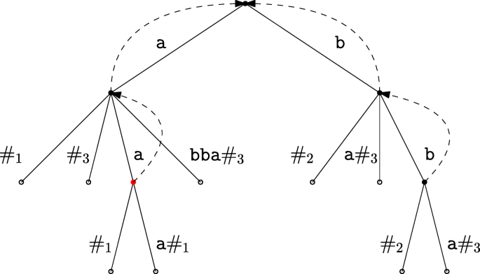

    

    The red node in the tree marks the path-label aa where $\texttt {aa} \in \mathrm {M}^{\ell }_{y_{N}}$. By traversing the leaves of this node, it is clear that aa is a proper factor of the first element aaa in $\mathrm {M}^{\ell }_{\{y_1,\ldots ,y_{N-1}\}}$

  • (b) We next want to check if the words y_N[i₁..i₂] ⋅ α are superwords of at least one element of $\mathrm {M}^{\ell }_{\{y_1,\ldots ,y_{N-1}\}}$. Recall that equality of words has already been checked in step 2(a). So we are just left with checking whether any element, say u, of $\mathrm {M}^{\ell }_{\{y_1,\ldots ,y_{N-1}\}}$ is a proper factor of y_N[i₁..i₂] ⋅ α. We rely on the following simple fact. If u is a proper factor of y_N[i₁..i₂] ⋅ α, then it is either a factor of the longest proper prefix of y_N[i₁..i₂] ⋅ α or a factor of the longest proper suffix of y_N[i₁..i₂] ⋅ α or of both. By definition of MAWs, y_N[i₁..i₂] ⋅ α can be represented by < i₁,i₂,α > or, equivalently, by < β,j₁,j₂ >, where α,β are letters, [i₁,i₂],[j₁,j₂] are intervals over y_N and y_N[i₁..i₂] ⋅ α = β ⋅ y_N[j₁..j₂]. The latter of the two representations can be obtained from the former using a batch of weighted ancestor queries similar to step 2(a) in linear time for all words in $\mathrm {M}^{\ell }_{y_{N}}$. We use radixsort to sort all intervals [i₁,i₂] and run the matching statistics algorithm for y_N with respect to $\mathcal {T}(\mathrm {M}^{\ell }_{\{y_1,\ldots ,y_{N-1}\}})$. By definition, no element in $\mathrm {M}^{\ell }_{\{y_1,\ldots ,y_{N-1}\}}$ is a factor of another element in the same set. Thus, if a factor of y_N[i₁..i₂] corresponds to an element in $\mathrm {M}^{\ell }_{\{y_1,\ldots ,y_{N-1}\}}$, this can be located in $\mathcal {T}(\mathrm {M}^{\ell }_{\{y_1,\ldots ,y_{N-1}\}})$ while running the matching statistics algorithm. The whole process takes $\mathcal {O}(|y_{N}| + \| \mathrm {M}^{\ell }_{\{y_1,\ldots ,y_{N-1}\}}\| )$ time: $\mathcal {O}(\| \mathrm {M}^{\ell }_{\{y_1,\ldots ,y_{N-1}\}}\| )$ time to construct the suffix tree and a further $\mathcal {O}(|y_{N}|)$ time for the matching statistics algorithm and for processing the $\mathcal {O}(|y_{N}|)$ tuples. We treat the case [j₁,j₂] analogously.

    Example 7

    Let ℓ = 3, $\mathrm {M}^{\ell }_{\{y_1,\ldots ,y_{N-1}\}}=\{\texttt {aaa,bb}\}$ and y_N = abba, so that $\mathrm {M}^{\ell }_{y_{N}}=\{\texttt {aa,bab,aba,bbb}\}$. We build the suffix tree of aaa#₁bb#₂ (see Fig. 3). We use identifiers in the form #_j where $j \in \{1, \ldots , |\mathrm {M}^{\ell }_{\{y_1,\ldots ,y_{N-1}\}}|$}. The sorted list of unique tuples from $\mathrm {M}^{\ell }_{y_{N}}$ is < 0, 0 >,< 0, 1 >,< 1, 2 >, < 2, 3 >. The longest match at position 0 of y_N = abba is a and there is no full match of a word from $\mathrm {M}^{\ell }_{\{y_1,\ldots ,y_{N-1}\}}$. We follow the suffix-link of the node, which takes us to the root. The longest match at position 1 is bb. This takes us to a full match of a word from $\mathrm {M}^{\ell }_{\{y_1,\ldots ,y_{N-1}\}}$ (bb), which means that bbb, whose prefix and suffix is represented by the single tuple < 1,2 >, is a superword of word bb from $\mathrm {M}^{\ell }_{\{y_1,\ldots ,y_{N-1}\}}$.

    Fig. 3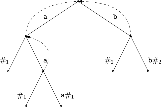

    

    Starting from the root, we find a path-label bb. The second element of $\mathrm {M}^{\ell }_{\{y_1,\ldots ,y_{N-1}\}}$ is a factor of word bbb in $\mathrm {M}^{\ell }_{y_{N}}$, whose prefix and suffix corresponds to the tuple < 1,2 >

  We create set $\mathrm {R}^{\ell }_{\{y_1,\ldots ,y_{N-1}\}}$ explicitly since it is a subset of $\mathrm {M}^{\ell }_{\{y_1,\ldots ,y_{N-1}\}}$. We create set $\mathrm {R}^{\ell }_{y_{N}}$ implicitly: every element $x \in \mathrm {R}^{\ell }_{y_{N}}$ is stored as a tuple < i₁,i₂,α > such that x = y_N[i₁..i₂] ⋅ α. We store every element of $\{x_{2}: x_{2} \in M \cap \mathrm {M}^{\ell }_{y_{N}}\}$ with the same representation. All other elements of M are stored explicitly.

• 3. Construct the suffix tree of y_N and use it to locate all occurrences of words in $\mathrm {R}^{\ell }_{\{y_1,\ldots ,y_{N-1}\}}$ in y_N and store the occurrences as pairs (starting position, ending position). This step can be carried out in time $\mathcal {O}(|y_{N}| + \| \mathrm {R}^{\ell }_{\{y_1,\ldots ,y_{N-1}\}}\| )$. This claim is due to the following fact: no element in $\mathrm {R}^{\ell }_{\{y_1,\ldots ,y_{N-1}\}}$ is a prefix of another element in $\mathrm {R}^{\ell }_{\{y_1,\ldots ,y_{N-1}\}}$.

• 4. For every i ∈ [1,N − 1], we perform the following to compute Case 2 MAWs:

  • (a) Read word y_i from memory. Construct the suffix tree T_x of word x = y_i#y_N in time $\mathcal {O}(|y_{i}| + |y_{N}|)$. Use T_x to locate all occurrences of elements of $\mathrm {R}^{\ell }_{y_{N}}$ in y_i and store the occurrences as pairs (starting position, ending position). This step can be completed in time $\mathcal {O}(|y_{i}| + |y_{N}|)$ similar to 2. This claim is due to the fact that no element in $\mathrm {R}^{\ell }_{y_{N}}$ is a prefix of another element in $\mathrm {R}^{\ell }_{y_{N}}$.

  • (b) During a bottom-up DFS traversal of T_x, we mark, at each explicit node of T_x, the smallest starting position of the word represented by that node, and the largest starting position of the same word. This can be done in time $\mathcal {O}(|y_{i}| + |y_{N}|)$ by propagating upwards the labels of the terminal nodes (starting positions of suffixes) and updating the smallest and largest positions analogously.

  • (c) Compute the set $\mathrm {M}^{\ell }_{y_{i}\#y_{N}}$ using [7], and output the words in the following constant-space form: < a,i₁,i₂,b > per word; such that a ⋅ x[i₁..i₂] ⋅ b is a MAW. This can be carried out in time $\mathcal {O}(|y_{i}| + |y_{N}|)$.

  • (d) For each element of $\mathrm {M}^{\ell }_{y_{i}\#y_{N}}$, we need to locate the node representing word ax[i₁..i₂] = au and the node representing word x[i₁..i₂]b = ub. This can be done in time $\mathcal {O}(|y_{i}| + |y_{N}|)$ via answering off-line a batch of weighted ancestor queries (Theorem 3). At this point, we have located the two nodes on T_x. We assign a pointer from the stored starting position g of au to the ending position f of ub (see Fig. 4), only if g is before # and f is after # (f can be computed using the stored starting position of ub and the length of ub). Conversely, we assign a pointer from the ending position f of ub to the stored starting position g of au, only if f is before # and g is after #.

    Fig. 4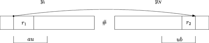

    

    au starts where a word r₁ of $\mathrm {R}^{\ell }_{y_{N}}$ starts in y_i and ub ends where a word r₂ of $\mathrm {R}^{\ell }_{\{y_1,\ldots ,y_{N-1}\}}$ ends in y_N

  • (e) Suppose au occurs in y_i and ub in y_N. We make use of the pointers as follows. Recall steps 3 and 4(a) and check whether au starts where a word r₁ of $\mathrm {R}^{\ell }_{y_{N}}$ starts and ub ends where a word r₂ of $\mathrm {R}^{\ell }_{\{y_1,\ldots ,y_{N-1}\}}$ ends. If this is the case , then by Theorem 1 aub is added to our output set M, otherwise we discard it. Inspect Fig. 4 in this regard. Conversely, if au occurs in y_N and ub in y_i, then we check whether au starts where a word r₂ of $\mathrm {R}^{\ell }_{\{y_1,\ldots ,y_{N-1}\}}$ starts and whether ub ends where a word r₁ of $\mathrm {R}^{\ell }_{y_{N}}$ ends. If this is the case, then aub is added to M, otherwise we discard it.

Finally, we set $\mathrm {M}^{\ell }_{\{y_1,\ldots ,y_N\}}=M$ as the output of the N th step. Let MaxIn be the length of the longest word in {y₁, … , y_k} and $\textsc {MaxOut}=\max \limits \{\| \mathrm {M}^{\ell }_{\{y_1,\ldots ,y_N\}}\| :N\in [1,k]\}$.

Theorem 4

Given k words y₁,y₂, … , y_k and an integer ℓ > 1, all $\mathrm {M}^{\ell }_{y_{1}},\ldots ,\mathrm {M}^{\ell }_{\{y_1,\ldots ,y_k\}}$ can be computed in $\mathcal {O}(kn+{\sum }^{k}_{N=1}\| \mathrm {M}^{\ell }_{\{y_1,\ldots ,y_N\}}\| )$ total time using $\mathcal {O}(\textsc {MaxIn}+\textsc {MaxOut})$ space, where $n={\sum }^{k}_{N=1}|y_{N}|$.

Proof

From the above discussion, the time is bounded by $\mathcal {O}({\sum }^{k}_{N=1}{\sum }^{N-1}_{i=1}(|y_{N}|+|y_{i}|)+{\sum }^{k}_{N=1}\| \mathrm {M}^{\ell }_{\{y_1,\ldots ,y_N\}}\| )$. We can bound the first term as follows.

$$ \begin{array}{@{}rcl@{}} && {\sum}^{k}_{N=1}{\sum}^{N-1}_{i=1}(|y_{N}|+|y_{i}|) \\ &\leq & {\sum}^{k}_{N=1}{\sum}^{k}_{i=1}(|y_{N}|+|y_{i}|)\\ &= & {\sum}^{k}_{N=1}{\sum}^{k}_{i=1}|y_{N}|+{\sum}^{k}_{N=1}{\sum}^{k}_{i=1}|y_{i}|\\ &= & 2k(|y_{1}|+\cdots+|y_{k}|). \end{array} $$

Therefore, the time is bounded by $\mathcal {O}(kn+{\sum }^{k}_{N=1}\| \mathrm {M}^{\ell }_{\{y_1,\ldots ,y_N\}}\| )$.

The space is bounded by the maximum time spent at a single step; namely, the length of the longest word in the collection plus the maximum total size of set elements across all output sets. Note that the total output size of the algorithm is the sum of all its output sets, that is ${\sum }^{k}_{N=1}\| \mathrm {M}^{\ell }_{\{y_1,\ldots ,y_N\}}\|$, and MaxOut could come from any intermediate set.

The correctness of the algorithm follows from Lemma 2 and Theorem 1. □

6 Proof-of-Concept Experiments

In this section, we do not directly compare against the fastest internal [7] or external [18] memory implementations because the former assumes that we have the required amount of internal memory, and the latter assumes that we have the required amount of external memory to construct and store the global data structures for a given input dataset. If the memory for constructing and storing the data structures is available, these linear-time algorithms are surely faster than the method proposed here. In what follows, we rather show that our output-sensitive technique offers a space-time tradeoff, which can be usefully exploited for specific values of ℓ, the maximal length of MAWs we wish to compute.

The time-efficient algorithm discussed in Section 5 (with the exception of storing and searching the reduced sets of words explicitly rather than in the constant-space form previously described) has been implemented in the C++ programming language¹. The correctness of our implementation has been confirmed against that of [7]. We have also implemented the algorithm discussed in Section 4 but as it was significantly slower, its results are omitted from here. As input datasets here we used: the entire human genome (version hg38), which has an approximate size of 3.1GB; the entire mouse genome (version mm10), which has an approximate size of 2.6GB; and the entire chimp genome (version panTro6), which has an approximate size of 2.8GB. All datasets were downloaded from the UCSC Genome Browser [26]. The following experiments were conducted on a machine with an Intel Core i5-4690 CPU at 3.50 GHz and 128GB of memory running GNU/Linux. We ran the program by splitting the genomes into k = 2,4,6,8,10 blocks and setting ℓ = 10,11,12. Figures 5, 6 and 7 depict the change in elapsed time and peak memory usage as k and ℓ increase (space-time tradeoff).

Fig. 5

Elapsed time and peak memory usage using increasing k blocks of the entire human genome (hg38) for ℓ = 10, 11, 12; notice that the peak memory usage is the same for all values of ℓ

Fig. 6

Elapsed time and peak memory usage using increasing k blocks of the entire mouse genome (mm10) for ℓ = 10,11,12; notice that the peak memory usage is the same for all values of ℓ

Fig. 7

Elapsed time and peak memory usage using increasing k blocks of the entire chimp genome (panTro6) for ℓ = 10,11,12; notice that the peak memory usage is the same for all values of ℓ

In accordance to Theorem 4: graph (a) in all figures shows an increase of time as k and ℓ increase; and graph (b) in all figures shows a decrease in peak memory as k increases. Notice that the space to construct the block-wise data structures bounds the total space used for the specific ℓ values and that is why the memory peak is essentially the same for the ℓ values used. This can specifically be seen for ℓ = 10 where all words of length 10 are present in all three genomes. The same datasets were used to run the fastest internal memory implementation for computing MAWs [7] on the same machine for ℓ = 12. Notice that the algorithm of [7] takes the same time and space irrespective of ℓ. It took only 2934 seconds to process the human genome but with a peak memory usage of 75.40GB (it took 2844 seconds to process the mouse genome with a peak memory usage of 66.54GB; and 2731 seconds to process the chimp genome with a peak memory usage of 69.49GB). These results confirm our theoretical findings and justify our contribution.

7 Final Remarks

We presented a new technique for constructing antidictionaries of long texts in output-sensitive space. Let us conclude with the following remarks:

• 1. Any space-efficient algorithm designed for global data structures (such as [20]) can be directly applied to the k documents in our technique to further reduce the working space.

• 2. There is a connection between MAWs and other word regularities [9]. Our technique could potentially be applied to computing these regularities in output-sensitive space.

• 3. Our technique could serve as a basis for a new parallelization scheme for constructing antidictionaries (see also [27]), in which several documents are processed concurrently.

References

Ayad, L A K, Badkobeh, G, Fici, G, Héliou, A., Pissis, S P: Constructing antidictionaries in output-sensitive space. In: Bilgin, A., Marcellin, M.W., Serra-Sagristà, J., Storer, J.A. (eds.) Data Compression Conference, DCC 2019, pp 538–547. IEEE, Snowbird (2019)
Crochemore, M, Mignosi, F, Restivo, A: Automata and forbidden words. Inf. Process. Lett. 67(3), 111–117 (1998)
Charalampopoulos, P, Crochemore, M, Fici, G, Mercas, R, Pissis, S P: Alignment-free sequence comparison using absent words. Inf. Comput. 262(1), 57–68 (2018)
Almirantis, Y, Charalampopoulos, P, Gao, J, Iliopoulos, C S, Mohamed, M, Pissis, S P, Polychronopoulos, D: On avoided words, absent words, and their application to biological sequence analysis. Algorithm. Mol. Biol. 12(1), 5:1–5:12 (2017)
Fici, G, Gawrychowski, P: Minimal absent words in rooted and unrooted trees. In: String Processing and Information Retrieval - 26th International Symposium, SPIRE 2019. Proceedings, Segovia (2019)
Fukae, H, Ota, T, Morita, H: On fast and memory-efficient construction of an antidictionary array. In: Proceedings of the 2012 IEEE International Symposium on Information Theory, pp. 1092–1096, IEEE (2012)
Barton, C, Héliou, A., Mouchard, L, Pissis, S P: Linear-time computation of minimal absent words using suffix array. BMC Bioinform. 15, 388 (2014)
Fujishige, Y, Tsujimaru, Y, Inenaga, S, Bannai, H, Takeda, M: Computing DAWGs and minimal absent words in linear time for integer alphabets. In: Faliszewski, P., Muscholl, A., Niedermeier, R. (eds.) 41st International Symposium on Mathematical Foundations of Computer Science, MFCS 2016, LIPIcs, vol. 58, pp 38:1–38:14. Schloss Dagstuhl - Leibniz-Zentrum fuer Informatik, Kraków (2016)
Charalampopoulos, P, Crochemore, M, Pissis, S P: On extended special factors of a word. In: Gagie, T., Moffat, A., Navarro, G., Cuadros-Vargas, E. (eds.) String Processing and Information Retrieval - 25th International Symposium, SPIRE 2018, Lima, Proceedings, Lecture Notes in Computer Science, vol. 11147, pp 131–138. Springer (2018)
Belazzougui, D, Cunial, F, Kärkkäinen, J., Mäkinen, V.: Versatile succinct representations of the bidirectional Burrows-Wheeler transform. In: Bodlaender, H.L., Italiano, G.F. (eds.) Algorithms - ESA 2013 - 21st Annual European Symposium, Sophia Antipolis. Proceedings, Lecture Notes in Computer Science, vol. 8125, pp 133–144. Springer (2013)
Belazzougui, D, Cunial, F: A framework for space-efficient string kernels. Algorithmica 79(3), 857–883 (2017)
Crochemore, M, Mignosi, F, Restivo, A, Salemi, S: Data compression using antidictionaries. Proc. IEEE 88(11), 1756–1768 (2000)
Crochemore, M, Navarro, G: Improved antidictionary based compression. In: 22nd International Conference of the Chilean Computer Science Society (SCCC 2002), pp. 7–13, Copiapo (2002)
Fiala, M, Holub, J: DCA using suffix arrays. In: 2008 data compression conference (DCC 2008), pp. 516. IEEE Computer Society, Snowbird (2008)
Ota, T, Morita, H: On the adaptive antidictionary code using minimal forbidden words with constant lengths. In: Proceedings of the International Symposium on Information Theory and its Applications, ISITA 2010, pp. 72–77. IEEE, Taichung (2010)
Crochemore, M, Héliou, A., Kucherov, G, Mouchard, L, Pissis, SP, Ramusat, Y: Minimal absent words in a sliding window and applications to on-line pattern matching. In: Klasing, R, Zeitoun, M (eds.) Fundamentals of Computation Theory - 21st International Symposium, FCT 2017, Bordeaux, Proceedings, Lecture Notes in Computer Science, vol. 10472, pp 164–176. Springer (2017)
Silva, RM, Pratas, D, Castro, L, Pinho, AJ, Ferreira, P J SG: Three minimal sequences found in Ebola virus genomes and absent from human DNA. Bioinformatics 31(15), 2421–2425 (2015)
Héliou, A., Pissis, SP, Puglisi, SJ: emMAW: computing minimal absent words in external memory. Bioinformatics 33(17), 2746–2749 (2017)
Kärkkäinen, J., Kempa, D, Puglisi, SJ: Parallel external memory suffix sorting. In: Cicalese, F., Porat, E., Vaccaro, U. (eds.) Combinatorial Pattern Matching - 26th Annual Symposium, CPM 2015, Ischia Island, Proceedings, Lecture Notes in Computer Science, vol. 9133, pp 329–342. Springer (2015). https://doi.org/10.1007/978-3-319-19929-0_28
Fujishige, Y, Takagi, T, Hendrian, D: Truncated DAWGs and their application to minimal absent word problem. In: Gagie, T., Moffat, A., Navarro, G., Cuadros-Vargas, E. (eds.) String Processing and Information Retrieval - 25th International Symposium, SPIRE 2018, Lima, Proceedings, Lecture Notes in Computer Science, vol. 11147, pp 139–152. Springer (2018)
Crochemore, M, Hancart, C, Lecroq, T: Algorithms on strings. Cambridge University Press (2007)
Farach, M: Optimal suffix tree construction with large alphabets. In: 38th Annual Symposium on Foundations of Computer Science, FOCS ’97, pp. 137–143. IEEE Computer Society, Miami Beach (1997)
Gusfield, D: Algorithms on strings, trees, and sequences: Computer science and computational biology. Cambridge University Press, New York (1997)
Farach, M, Muthukrishnan, S: Perfect hashing for strings: Formalization and algorithms. In: Hirschberg, D.S., Myers, E.W. (eds.) Combinatorial Pattern Matching, 7th Annual Symposium, CPM 96, Laguna Beach, Proceedings, Lecture Notes in Computer Science, vol. 1075, pp 130–140. Springer (1996)
Kociumaka, T, Kubica, M, Radoszewski, J, Rytter, W, Walen, T: A linear-time algorithm for seeds computation. ACM Trans. Algorithm. 16(2), 27:1–27:23 (2020)
Kent, WJ, Sugnet, CW, Furey, TS, Roskin, KM, Pringle, TH, Zahler, AM, Haussler, D: The human genome browser at UCSC. Genome Res. 12(6), 996–1006 (2002)
Barton, C, Héliou, A., Mouchard, L, Pissis, SP: Parallelising the computation of minimal absent words. In: Wyrzykowski, R., Deelman, E., Dongarra, J.J., Karczewski, K., Kitowski, J., Wiatr, K. (eds.) Parallel processing and applied mathematics - 11th international conference, PPAM 2015, Krakow. revised selected papers, part II, Lecture Notes in Computer Science, vol. 9574 , pp 243–253. Springer (2015)
Gagie, T, Moffat, A, Navarro, G, Cuadros-Vargas, E. (eds.): String processing and information retrieval - 25th international symposium, SPIRE 2018, Lima, proceedings, Lecture Notes in Computer Science, vol. 11147 Springer (2018)
Funding
Open access funding provided by Università degli Studi di Palermo within the CRUI-CARE Agreement.
Author information
Authors and Affiliations
Corresponding author
Additional information
Publisher’s Note
Springer Nature remains neutral with regard to jurisdictional claims in published maps and institutional affiliations.
A preliminary version of this paper was presented at the Data Compression Conference 2019 [1] . Gabriele Fici is supported by MIUR-PRIN 2017 project “Algorithms, Data Structures and Combinatorics for Machine Learning”.
Rights and permissions
Open Access This article is licensed under a Creative Commons Attribution 4.0 International License, which permits use, sharing, adaptation, distribution and reproduction in any medium or format, as long as you give appropriate credit to the original author(s) and the source, provide a link to the Creative Commons licence, and indicate if changes were made. The images or other third party material in this article are included in the article's Creative Commons licence, unless indicated otherwise in a credit line to the material. If material is not included in the article's Creative Commons licence and your intended use is not permitted by statutory regulation or exceeds the permitted use, you will need to obtain permission directly from the copyright holder. To view a copy of this licence, visit http://creativecommons.org/licenses/by/4.0/.
About this article
Cite this article
Ayad, L.A., Badkobeh, G., Fici, G. et al. Constructing Antidictionaries of Long Texts in Output-Sensitive Space. Theory Comput Syst 65, 777–797 (2021). https://doi.org/10.1007/s00224-020-10018-5
Accepted:
Published:
Issue Date:
DOI: https://doi.org/10.1007/s00224-020-10018-5